How Wide is the Transition to Deconfinement?

Abstract

Pure $SU(3)$ glue theories exhibit a deconfining phase transition at a nonzero temperature, $T_{c}$. Using lattice measurements of the pressure, we develop a simple matrix model to describe the transition region, when $T\geq T_{c}$. This model, which involves three parameters, is used to compute the behavior of the ’t Hooft loop. There is a Higgs phase in this region, where off diagonal color modes are heavy, and diagonal modes are light. Lattice measurements of the latter suggests that the transition region is narrow, extending only to about $\sim 1.2\,T_{c}$. This is in stark contrast to lattice measurements of the renormalized Polyakov loop, which indicates a much wider width. The possible implications for the differences in heavy ion collisions between RHIC and the LHC are discussed.

Heavy ion collisions at the Relativistic Heavy Ion Collider (RHIC) have demonstrated a rich variety of unexpected behavior hydro . Notably, in peripheral collisions the elliptical flow can only be described by nearly ideal hydrodynamics, with a very small ratio between the shear viscosity, $\eta$, and the entropy density, $s$. The differences between collisions at RHIC, and those which will soon be observed soon at the Large Hadron Collider (LHC), will be especially interesting: does the nearly ideal hydrodynamic behavior, observed at RHIC, persist at the much higher energies of the LHC?

One approach to deconfinement exploits the analogy to ${\cal N}=4$ supersymmetric gauge theories: using the AdS/CFT correspondence, such theories are computable analytically in the limit of infinite coupling, for an infinite number of colors ads_reviews . By introducing a potential for the dilation field, the behavior of the entropy density near the deconfining phase transition, at a temperature $T_{c}$, can be fit from measurements on the lattice gubser ; kiritsis ; other ; gyulassy . While the entropy density, $s$, decreases strongly as $T\rightarrow T_{c}^{+}$ because it is related to Hawking radiation, in AdS/CFT models the ratio $\eta/s$ remains completely independent of temperature. This suggests that like RHIC, that collisions at the LHC should also be described by nearly ideal hydrodynamics; see, also, Ref. shuryak .

In this work we consider a very different approach to the deconfining phase transition. It assumes that the coupling is moderate even down to the transition temperature, $T_{c}$ laine . We use an elementary matrix model, involving three parameters, to parametrize the behavior of the deconfining phase transition. A version of this model with one parameter was first proposed by Meisinger, Miller, and Ogilvie ogilvie1 . Similar models arise for theories in which one (or more) spatial directions are of femtoscale size ogilvie2 ; ogilvie3 ; matrix_other ; aharony .

The parameters of the model are fixed from lattice measurements of the pressure pressure2 ; pressure3 ; panero ; pressure_dyn . It then predicts how the ’t Hooft loop interface1 ; interface2 ; interface3 ; interface4 ; interface5 changes with temperature near $T_{c}$, which we compare to the results of lattice simulations interface_lattice1 ; interface_lattice2 . Further, the model predicts that for a range of temperatures above $T_{c}$, there is a Higgs phase, where correlation functions of electric fields are a mixture of heavy and light modes, from fields which are off diagonal, and diagonal, in color, respectively. This may help to understand the results of lattice simulations pressure3 ; gauge_inv_mass_su3 ; gauge_inv_mass_su2 ; gluon_mass_1 , which are otherwise somewhat puzzling.

The most direct prediction of our model is for the expectation value of the Polyakov loop. For the pure glue $SU(3)$ theory, lattice simulations find that the (renormalized) Polyakov loop vanishes below $T_{c}$, jumps to $\sim 0.4$ at $T_{c}^{+}$, and then rises with $T$, until it is approximately constant above $\sim 4.0\,T_{c}$ ren_loop1 ; ren_loop2 ; ren_loop3 . This represents confinement below $T_{c}$, a complete Quark Gluon Plasma (QGP) at high temperature, and a “semi”-QGP in between semi1 ; semi2 ; higgs ; yk . Physically, there is no ionization of color in the confined phase, total ionization in the complete QGP, and only partial ionization in the semi-QGP yk . (While we discuss a purely gluonic plasma, we adopt the common term QGP.)

The principal thrust of this paper is that from indirect measurements on the lattice, we suggest that the width of the semi-QGP is much narrower than indicated by present results for the renormalized Polyakov loop: not up to $\sim 4.0\,T_{c}$, but only $\sim 1.2\,T_{c}$. We do not understand this discrepancy in detail, but suggest a possible reason later. This discrepancy is the reason why, having fit the parameters of our model from the pressure, we compute both the ’t Hooft loop and gluon masses.

While we treat the pure glue theory, our model can be extended to QCD, with dynamical quarks pressure_dyn . It is reasonable to assume that in QCD, the semi-QGP is like that of the pure glue theory, relatively narrow. We thus conclude by discussing the possible phenomenological implications of our results for heavy ion collisions.

How confinement arises in our model can be understood by analogy. For a bosonic field, with energy $E$ and chemical potential $\mu$, the Bose-Einstein statistical distribution function is

$$n(E,q)=\frac{1}{{\rm e}^{(E-\mu)/T}-1}=\frac{1}{{\rm e}^{E/T-2\pi iq}-1}\;.$$ (1)

Instead of taking $\mu$ to be real, as in ordinary thermodynamical systems, for the purposes of the analogy we take it to be purely imaginary, and define $\mu=2\pi T\,i\,q$, where $q$ is real.

Doing so, $n(E,q)$ is clearly a periodic function of $q$, invariant under $q\rightarrow q+1$. Thus we can choose to define $q$ to lie within the range from $-\frac{1}{2}$ to $+\frac{1}{2}$.

Now assume that we integrate over $q$, with a distribution which is flat in $q$. Expand for large energy, so that the first term is the Boltzmann statistical distribution function. Given the assumed distribution in $q$, the integral of this term vanishes,

$${\rm e}^{-E/T}\;\int^{+1/2}_{-1/2}\;{\rm e}^{2\pi iq}\;dq=0\;.$$ (2)

Indeed, we can expand the Bose-Einstein distribution function term by term in powers of Boltzmann factors, ${\rm e}^{-E/T+2\pi iq}$ aharony ; doing so, the integral over each and every term obviously vanishes. The same is true for the Fermi-Dirac distribution function as well.

Thus a flat distribution in $q$ represents the confined phase. To represent a phase with partial deconfinement, one integrates over a limited region, say $q:-q_{0}\rightarrow+q_{0}$, with $q_{0}<\frac{1}{2}$. Complete deconfinement occurs when one integrates over a distribution which is a delta-function in $q$.

This example appears somewhat artificial. For a given $q$, the statistical distribution functions are complex valued, and so only integrals over $q$ can possibly represent physical quantities. Indeed, the grand canonical ensemble is characterized by a fixed value for the chemical potential, and not by an integral over $\mu$’s.

Nevertheless, precisely this mechanism arises for the deconfining phase transition in a $SU(N)$ gauge theory. Consider the expansion about a background field for the time-like component of the vector potential,

$$\left(A^{cl}_{0}\right)_{ab}=\frac{2\pi T}{g}\;q_{a}\;\delta^{ab}\;;$$ (3)

$a$ and $b$ are colors indices, running from $1\ldots N$. For nonzero $q_{a}$’s, this background field acts like an imaginary chemical potential for the diagonal elements of the gauge group. Integration over the $q_{a}$’s arises from imposing Gauss’ law for those elements of the gauge group interface2 .

This background field generates a non-trivial expectation for the Polyakov loop, $\ell$, which is the color trace of the thermal Wilson line, ${\bf L}$:

$$\ell=\frac{1}{N}\;{\rm tr}\,{\bf L}\;\;;\;\;{\bf L}={\cal P}\exp\left(ig\int^{1/T}_{0}A_{0}\;d\tau\right)\;;$$ (4)

$\cal P$ represents path ordering, $T$ is the temperature, and $\tau$ the imaginary time, $\tau:0\rightarrow 1/T$.

The lattice demonstrates that near $T_{c}$, the expectation value of the Polyakov loop is not near one, and decreases as the temperature does. In such a region, the eigenvalues of the logarithm of the thermal Wilson line are nonzero. Taking an ansatz such as Eq. (3) is the simplest possible way to model this. We do not attempt to derive the distribution of these eigenvalues, but to guess that from lattice results.

Since the gauge potential $A_{0}$ is an element of $SU(N)$, $\sum_{a=1}^{N}q_{a}=0$, modulo one, there are $N-1$ independent $q_{a}$’s. At infinite $N$, the $q_{a}$’s form a continuum, and the example of Eq. (1) is exact; see, e.g., computations on a femtosphere at $N=\infty$ aharony . For two colors, we can choose the eigenvalues to be $q_{1}=-q_{2}$; for three, $q_{1}=-q_{2}$, and $q_{3}=0$.

In the presence of the background field of Eq. (3), a potential for the $q_{a}$’s is generated at one loop order interface1 ; interface2 ; interface3 ; interface4 ; interface5 ,

$${\cal V}_{pt}(q_{a})\;=\;\frac{2\pi^{2}T^{4}}{3}\;\sum_{a,b=1}^{N}\;q_{ab}^{2}\left(1-|q_{ab}|\right)^{2}-\;(N^{2}-1)\frac{\pi^{2}T^{4}}{45}\;.$$ (5)

where $q_{ab}=q_{a}-q_{b}$, defined modulo one. The minimum is at $q_{a}=0$, where $-{\cal V}_{pt}(0)$ is the pressure for an ideal gas of gluons.

The potential ${\cal V}_{pt}(q_{a})$ enters in computations of the ’t Hooft loop. It is useful to consider deconfinement as a type of spin system. A pure $SU(N)$ gauge theory has $N$ degenerate vacua, where the thermal Wilson line $\bf L$ equals one of the $N$ roots of unity,

$${\bf L}={\rm e}^{2\pi ij/N}\;{\bf 1}\;,$$ (6)

$j=0\ldots(N-1)$. The usual vacuum, with $j=0$ and ${\bf L}={\bf 1}$, corresponds to all $q_{a}=0$. A $Z(N)$ vacua with $j=1$ and ${\bf L}={\rm e}^{2\pi i/N}{\bf 1}$ corresponds to $N-1$ $q_{a}$’s $=1/N$, and the remaining element $=-1+1/N$.

At high temperature in the complete QGP, the theory lies in one spin state, which we can choose to be $j=0$. One can compute tunneling between two degenerate vacua by constructing a box which is long in one spatial direction, with $j=0$ at one end, and $j=1$ at the other. An interface between the two ordered states forms in the center of the box, with the interface tension between the two computable semi-classically, using the potential ${\cal V}_{pt}(q_{a})$ interface1 ; interface2 ; interface3 ; interface4 ; interface5 . This interface is equivalent to a ’t Hooft loop which wraps around the center of the box interface3 .

As the temperature decreases and $T$ approaches $T_{c}$, domains with $j\neq 0$ form and grow in size. They become increasingly probable, until at $T_{c}^{-}$ and below, as a spin system the vacuum is completely disordered, a sum over many spin domains.

We want to add terms to the effective potential which model the transition to deconfinement. We could add perturbative corrections to ${\cal V}_{pt}(q_{a})$, which have been computed to $\sim g^{3}$ interface4 , but invariably they give $q_{a}=0$ (or a $Z(N)$ equivalent state) as the vacuum. With a complete theory, such as the monopole model of Liao and Shuryak shuryak , this potential could be computed directly.

We adopt a more modest approach, attempting to guess the form of the non-perturbative potential. We fit the coefficients which enter to lattice results for the pressure, and then use it to compute other quantities. The advantage of our approach is that we can compute quantities not just in, but near thermal equilibrium. Such quantities, like the shear viscosity yk , are much harder to extract on the lattice.

Since the Polyakov loop is an order parameter for deconfinement, a natural guess is that the non-perturbative potential involves $Z(N)$ invariant elements of the Lie group. The first such term is the adjoint loop matrix_other ; semi1 ; semi2 ; higgs ; yk ; lattice_eff ; pnjl . Instead, following the authors of Ref. ogilvie1 , and computations of the ’t Hooft loop interface1 ; interface2 ; interface3 ; interface4 ; interface5 , we write a potential which is a polynomial in the $q_{a}$’s.

There are several symmetries which any potential of the $q_{a}$’s must satisfy. It must be periodic in each $q_{a}$, with $q_{a}\rightarrow q_{a}+1$. It must also be invariant under $Z(N)$ transformations, where $N-1$ of the $q_{a}$’s shift by $1/N$, and the last element, by $-1+1/N$. Lastly, if we interchange the ordering of the $q_{a}$’s, we can change $q_{ab}\rightarrow q_{ba}=-q_{ab}$. These symmetries can be satisfied by constructing a potential as a function of $q_{ab}(1-q_{ab})$.

We can still form an infinite number of terms by tying together the color indices in different ways; see, e.g., the examples at two interface4 and three aharony loop order. We adopt the simplest approach, and take terms like those which arise at one loop order, Eq. (5), which involve a sum over one $q_{ab}$:

$${\cal V}_{non}(q_{a})=T^{2}\;T_{c}^{2}\;\sum_{a,b=1}^{N}\left(c_{1}\;|q_{ab}|(1-|q_{ab}|)\right.$$

$$\left.+c_{2}\;q_{ab}^{2}\left(1-|q_{ab}|\right)^{2}+c_{3}\right)\;.$$ (7)

The model of Ref. ogilvie1 involves terms $\sim c_{1}$ and $c_{3}$; these are kept in fixed ratio, given by the second Bernoulli polynomial. Instead, we allow $c_{1}$ and $c_{3}$ to vary independently. This helps to avoid a pathology of the model of Ref. (ogilvie1 ), where the pressure is negative at $T_{c}$.

We also introduce a term $\sim c_{2}\,q_{ab}^{2}(1-q_{ab})^{2}$; this is proportional to the perturbative term in Eq. (5), and is related to the fourth Bernoulli polynomial.

We take all of the non-perturbative terms to be $\sim T^{2}$, since lattice simulations indicate that in the pure glue theory, the leading corrections to terms $\sim T^{4}$ are $\sim T^{2}$ ogilvie1 ; ogilvie2 ; higgs ; fuzzy . There is obviously no fundamental reason why other terms, such as those $\sim 1$, could not also appear.

When the $q_{a}$’s develop an expectation value, this represents symmetry breaking for an adjoint scalar field, $A_{0}$, coupled to an $SU(N)$ gauge field, the $A_{i}$’s higgs . As an adjoint scalar, though, there is no strict order parameter which distinguishes between the symmetric and broken phases. Thus there need not be a phase transition in going from the symmetric phase, the complete QGP, to the “broken” phase, the semi-QGP.

If there were such a phase transition, it would represent a second transition, above $T_{c}$, separate from that for deconfinement. While possible, in a pure $SU(N)$ gauge theory lattice simulations only find evidence for one phase transition, at $T_{c}$ pressure2 ; pressure3 ; panero ; pressure_dyn . To avoid a phase transition between the complete and semi-QGP, it is essential that the non-perturbative potential has a term which is linear in the $q_{a}$’s. Assume that the effective potential only involved terms such as $\sim q_{ab}^{n}(1-q_{ab})^{n}$ for $n\geq 2$. For small $q_{a}$, these are of quadratic or higher order in the $q_{a}$’s, and of necessity, there would then be a phase transition when the $q_{a}$’s developed a nonzero expectation value. This transition might be of either first or second order, but there would be a phase transition. When $c_{1}\neq 0$, though, a term linear in the $q_{a}$’s ensures that there is no such phase transition. Instead, even for high temperature, there is always a small but non-zero expectation value for the $q_{a}$’s, $<q_{a}>\,\sim 1/T^{2}$; that is, the theory is always in a Higgsed phase. As we shall see however, this point is somewhat academic. For the parameters relevant to two and three colors, the region in which Higgsing matters is very narrow.

We remark that effective theories on the lattice often exhibit phases with broken symmetry lattice_higgs . The necessity of such a broken phase near $T_{c}$ does not seem to have been appreciated previously, though.

To determine the parameters of the model we compare to lattice measurements of the pressure. For three colors, this is illustrated in Fig. (1); for two colors, in Fig. (2). If $p(T)$ is the pressure, and $e(T)$ the energy density, then a more sensitive test of the fit is also to plot the interaction measure, $\Delta=e-3p$. Thus in each figure we plot $p/T^{4}$, $e/T^{4}$, and $\Delta/T^{4}$, both from the lattice, from Ref. (pressure2 ) for two colors, and from Ref. (pressure3 ) for three colors.

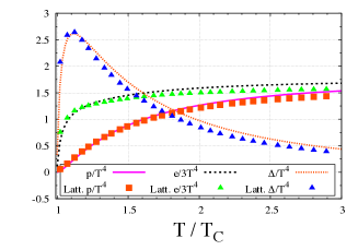
Figure 1: Comparison of lattice results for $SU(3)$ pure gauge to the model, for the pressure, energy density, and interaction measure.

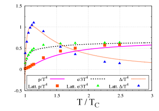
Figure 2: Comparison of lattice results for $SU(2)$ pure gauge theory to the model, for the pressure, energy density, and interaction measure.

The parameters of the fit are

$$c_{1}=-\,.41488\,;\,c_{2}=-\,5.45957\,;\,c_{3}=0.21954\,.$$ (8)

for three colors, and

$$c_{1}=-\,0.30267\,;\,c_{2}=-\,5.97440\,;\,c_{3}=0.18341\,.$$ (9)

for two colors.

While our model appears to involve three parameters, this is misleading. One parameter fixes the critical temperature, $T_{c}$. A second is chosen so that the pressure vanishes at $T_{c}$. Thus we really have only one free parameter, which is tuned to fit the behavior of the pressure near $T_{c}$.

For two colors, our model exhibits unphysical behavior, as the energy density is negative below $\sim 1\%$ of $T_{c}$. This might be corrected by adding further terms in the nonperturbative potential, such as higher Bernoulli polynomials.

In any case, since we fix the pressure to vanish at $T_{c}$, within our approximations the confined phase has vanishing pressure. How to match to a more realistic description of the confined phase is an important problem, which we defer for now.

Given the effective Lagrangian, it is then straightforward to compute the ’t Hooft loop. In the complete QGP, the potential includes only the perturbative potential, ${\cal V}_{pt}(q_{a})$, Eq. (5); in the semi-QGP, it is a sum of this and the non-perturbative potential, ${\cal V}_{non}(q_{a})$.

For two colors, as $q_{2}=-q_{1}$ there is only one independent direction, and it is direct to compute the tunneling path, and its associated action, analytically. The result for the ’t Hooft loop is

$$\sigma(T)=\frac{4\pi^{2}T^{2}}{3\sqrt{6g^{2}(T)}}\;\xi(g^{2})\;\frac{(1-(T_{c}/T)^{2})^{3/2}}{1-0.908\,(T_{c}/T)^{2}}\;,$$ (10)

where

$$\xi(g^{2})=1-0.16459\,g^{2}(T)\;.$$

The factors involving $T_{c}/T$ are special to the semi-QGP, so that as $T\gg T_{c}$, the result reduces to that in the complete QGP interface1 . The function $\xi(g^{2})$ is the correction $\sim g^{2}$ in the complete QGP; in plotting, we take $g^{2}(2\pi T)$ laine .

The ’t Hooft loop vanishes at $T_{c}$, as expected for a second order phase transition. From universality, the result in the Ising model is $\sigma(T)\sim(T-T_{c})^{2\nu}$, with $2\nu\sim 1.26$; lattice results in a gauge theory interface_lattice1 find $2\nu\sim 1.32$ interface_lattice1 . Our result, $2\nu=1.5$, is not too far off, as expected for a mean field theory. We note, however, that because of the term in the denominator, that the numerical agreement isn’t close. This is presumably related to the unphysical behavior of the energy density near $T_{c}$, mentioned previously.

For three colors, in the semi-QGP the vacua is along $\lambda_{3}$ (using the Gell-Mann notation), while the path for the ’t Hooft loop depends upon a change in $\lambda_{8}$. The path was determined numerically, and lies along both $\lambda_{3}$ and $\lambda_{8}$. The action of the tunneling path was also determined numerically, and the result for the ’t Hooft loop for three colors is illustrated in Fig. (3). (For $N=2$, we take $T_{c}/\Lambda_{\bar{MS}}=1.31$; for $N=3$, $1.14$. For the same value of $T_{c}/\Lambda_{\bar{MS}}=1.31$, the results unexpectedly coincide.)

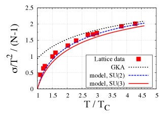
Figure 3: The ’t Hooft loop for $SU(3)$ pure gauge theory: lattice data from Ref. interface_lattice2 , and GKA, Giovannangeli and Korthals Altes, Ref. interface4 , the semi-classical computation in the complete QGP, including corrections of $\sim g^{2}$. In our model we show results for two and three colors, assuming that the corrections of $\sim g^{2}$ are identical in the complete and semi-QGP; see text.

Including $\xi(g^{2})$, the semi-classical computation of the ’t Hooft loop in the complete QGP agrees with lattice simulations above $\sim 4.0\,T_{c}$; below that temperature, they agree with the result in the semi-QGP interface_lattice2 . To obtain agreement, however, it is necessary to include the correction $\xi(g^{2})$; this is computed in the complete QGP, which is incorrect. Two things are required to compute $\xi(g^{2})$ in the semi-QGP. First, the potential for constant $q_{a}$ needs to be computed to two loop order, expanding about the full potential, ${\cal V}_{pt}(q_{a})+{\cal V}_{non}(q_{a})$. Second, corrections to one loop order need to be computed for the kinetic term. In the complete QGP this brings in new functions, the $\psi(q_{a})$ interface1 . Other functions could arise in the semi-QGP. For now, we defer these involved computations; since the corrections $\sim g^{2}$ are large, $\sim 50\%$, our results should be considered as tentative.

Besides the ’t Hooft loop, which is an interface tension for an order-order interface at $T\geq T_{c}$, the interface tension for the order-disorder interface, at $T_{c}$, is also computable in our model. This only exists for a first order transition; for three colors,

$$\sigma_{dis}=0.0258012\;\frac{T_{c}^{2}}{\sqrt{g^{2}}}\;.$$ (11)

It is necessary to compute the corrections $\sim g^{2}$ before comparing to lattice data, though.

The parameters for three colors, Eq. (8), and two colors, Eq. (9), are similar; the difference is commensurate with a dependence on $\sim 1/N^{2}$, with the coefficient of order one. We have then assumed that the parameters for three colors are close to those for higher $N$. We find reasonable agreement for the interaction measure to lattice results panero . When $N\geq 4$, there is more than one ’t Hooft loop. Lattice simulations find that they obey Casimir scaling to good approximation interface_lattice2 . We have not checked this explicitly, but suspect that in our model, ’t Hooft loops respect Casimir scaling.

The most novel prediction of our model is that there is a Higgs effect in the semi-QGP. This was noted first in Ref. higgs , and in theories at a femtoscale matrix_other . To understand it, consider the quantum fluctuations about the background field of Eq. (3):

$$\left\langle\left(A_{0}^{qu}\right)_{ab}(\vec{x})\,\left(A_{0}^{qu}\right)_{ba}(0)\right\rangle\sim\int\frac{d^{3}p}{(2\pi)^{3}}\;{\rm e}^{i\vec{p}\cdot\vec{x}}\sum_{n=-\infty}^{+\infty}\Delta_{00}$$ (12)

where $\Delta_{00}$ is the quantum propagator

$$\Delta_{00}=\frac{{\rm e}^{-ip_{0}\tau}}{(\vec{p}\,)^{2}+p_{0}^{2}+m_{\rm D}^{2}(q)}\,;\,p_{0}=2\pi T\left(n+q_{a}-q_{b}\right)\;.$$ (13)

The shift in the energy, $p_{0}=2\pi Tn\rightarrow 2\pi T(n+q_{a}-q_{b})$, is because we are expanding about a background field. The background field $A_{0}^{cl}$ acts upon quantum fluctuations like an adjoint Higgs field. Because the field is diagonal in color, Eq. (3), diagonal fields do not feel the background field. Thus for diagonal fields, the only mass they develop is the Debye mass, $m_{\rm D}$. This is of order $\sim gT$ times a function of the $q_{a}$’s yk . In contrast, off diagonal fields have non-trivial commutators with a diagonal field, and so they develop “masses” which are large, $\sim 2\pi T(n+q_{a}-q_{b})$.

We illustrate this in Fig. (4) for three colors. The masses of the two diagonal gluons are equal, and decrease as $T\rightarrow T_{c}^{+}$. There are two types of off-diagonal gluons: four with $|a-b|=1$, and two with $|a-b|=2$. The splitting of the masses is evident only close to $T_{c}$, for $T<1.2\,T_{c}$.

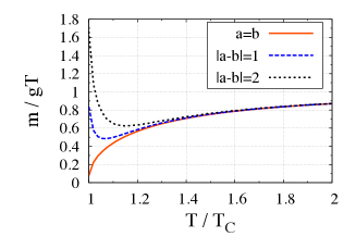
Figure 4: Gluon masses, $m_{ab}/(gT)$, for $SU(3)$ pure gauge theory: diagonal gluons, with $a=b$, are light; while there are two off diagonal gluons with heavy masses, for $|a-b|=1$ and $|a-b|=2$.

We do not plot lattice data, because it is somewhat contradictory. Lattice measurements of a gauge invariant quantity, the two point function between Polyakov loops, shows that the associated mass decreases as $T\rightarrow T_{c}^{+}$ pressure3 . In contrast, the two point function of gluons indicate that the gauge dependent mass increases as $T\rightarrow T_{c}^{+}$ gluon_mass_1 . Clearly it would be best to reanalyze the lattice data with a Higgsed propagator in the effective theory, Eq. (13), with its characteristic combination of modes whose masses both increase and decrease.

The static, spatial gluon fields, the $A_{i}$, also undergo a Higgs effect. This happens as well in a monopole gas shuryak .

We have not discussed the most obvious application of our model: the computation of the Polyakov loop. We plot this quantity, and the lattice results, for three colors in Fig. (5).

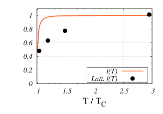
Figure 5: The Polyakov loop for a $SU(3)$ pure gauge theory from lattice simulations ren_loop3 and in our model.

A direct comparison of the two is somewhat misleading. We have not computed perturbative corrections to the Polyakov loop, which enter at $\sim g^{3}$ pert_ren_loop . This contribution is positive, and will increase the result. Nevertheless, while the two coincide at $T_{c}$ — which is presumably coincidence — they immediately diverge from one another. From Fig. (5), in our model the loop quickly goes up to a constant value by $\sim 1.2\,T_{c}$; this is very different from lattice measurements, for which it is not constant until a much higher temperature, $\sim 4.0\,T_{c}$ ren_loop1 ; ren_loop2 ; ren_loop3 .

If our model is correct, why does the value of the Polyakov loop, computed from our model, differ so significantly from lattice measurements of the (renormalized) Polyakov loop? There is an ambiguity associated with the renormalized Polyakov loop, from the zero point energy. In Ref. yk we argued that perturbatively, the zero point energy vanishes for a straight Polyakov loop. This argument fails for a “smeared” loop (see, e.g., the appendix of Ref. ren_loop2 ). If so, then the effects of smearing must be very dramatic.

We comment that a similar rapid growth in the Polyakov loop is found in solutions of the Schwinger-Dyson equations pawlowski . Our results do not coincide numerically, though.

To understand our results better, consider first the limit of intermediate temperature: say above $\sim 1.5\,T_{c}$, and up to $\sim 4.0\,T_{c}$. In this limit the $q_{a}$’s are small. As noted before, for small $q$ the dominant terms are $\sim c_{1}T^{2}q$ in the nonperturbative potential, Eq. (7), and that $\sim T^{4}q^{2}$ in the perturbative potential, Eq. (5). Balancing these two gives $\langle q_{a}\rangle\sim-c_{1}/\pi^{2}(T_{c}/T)^{2}$; for three colors, $\langle q_{a}\rangle\sim 0.04\,(T_{c}/T)^{2}$. Thus while the theory is nominally always in a “Higgsed” phase, as a practical matter this effect is numerically miniscule. Further, since the loop involves the cosine of the $q_{a}$’s, asymptotically the deviation of the loop from unity is even smaller: $1-\ell\sim q^{2}\sim(T_{c}/T)^{4}$.

At intermediate temperatures, what is the origin of the term $\sim T^{2}$ in the pressure; or equivalently, the behavior of the interaction measure, $\Delta/T^{4}\sim 1/T^{2}$? If the $q\sim 1/T^{2}$, for small $q$ terms $\sim T^{4}q^{2}$ and $\sim T^{2}q$ are of order one. Then the only contribution to a term $\sim T^{2}$ in the pressure is from the $q$-independent terms in the nonperturbative potential. In our model, this is a single term, $\sim c_{3}\,T_{c}^{2}\,T^{2}$.

On the other hand, for intermediate temperatures, even if the pressure does not probe the other terms in the potential, the ’t Hooft loop does. By measuring a ’t Hooft loop, the altered boundary conditions force the system to probe the $q$-dependence of the potential in a nontrivial way. In the present model, these are determined by the coefficients for $c_{1}$ and $c_{2}$. (As a constant term, the value of $c_{3}$ doesn’t matter.) In this way the lattice measurements of the ’t Hooft loop interface_lattice1 ; interface_lattice2 are an absolutely essential constraint on our model.

In contrast, near $T_{c}$ all of the parameters of the model matter, contribute to both the behavior of the pressure and the value of the $q_{a}$’s. By comparison, consider the model of Ref. (ogilvie1 ), where $c_{2}=0$. We take two colors, since then the expressions are algebraically simple. From Ref. (ogilvie1 ), with $q=q_{1}=-q_{2}$,

$$q_{c_{2}=0}=\frac{1}{4}\left(1-\sqrt{1-\left(\frac{T_{c}}{T}\right)^{2}}\right)\;.$$ (14)

When $c_{2}=0$, though, the interaction measure is much broader than indicated by the lattice data.

In the present model, with $c_{1},c_{2}\neq 0$,

$$q=\frac{1}{4}\left(1-\sqrt{1+\frac{2c_{1}}{c_{2}+(2\pi^{2}/3)(T/T_{c})^{2}}}\right)\;.$$ (15)

The values of $c_{1}$ and $c_{2}$ are dictated by fitting the pressure, or more sensitively, the interaction measure. By making $c_{2}$ increasingly negative from $c_{2}=0$, one finds that the peak in the interaction measure becomes increasingly sharp. Since the loop vanishes at $T_{c}$ for two colors, $c_{1}$ is then adjusted so that $q=1/4$ at $T=T_{c}$.

Tuning $c_{2}$ and $c_{1}$ in this way, one finds that as the peak in the interaction measure sharpens, that the region in which $q$ is nonzero narrows as well. This is due to the particular values of our fit: near $T_{c}$, the term $\sim c_{2}T_{c}^{2}T^{2}$ is not only large, but approximately cancels the similar term, with coefficient $(2\pi^{2}/3)\,T^{4}$, in the perturbative potential. Requiring $q=1/4$ at $T=T_{c}$ fixes $c_{2}+2\pi^{2}/3=-2c_{1}$, so that $|c_{1}|$ is small, $|c_{1}|\ll|c_{2}|$. From Eq. (15), the combination $c_{1}/(c_{2}+(2\pi^{2}/3)(T_{c}/T)^{2})$ enters into $q$, and implies that it is much sharper than the corresponding factor, $(T/T_{c})^{2}$ for $c_{2}=0$, Eq. (14). A similar cancellation happens for three colors.

We suggest that this reflects real physics: the sharpness of the interaction measure reflects the narrowness of the region in which the loop deviates significantly from unity. For the model with $c_{2}=0$, Eq. (14), $q$ always exceeds the corresponding value in our model, with $c_{2}\neq 0$. This is also seen for $T\gg T_{c}$: when $c_{2}=0$, $q\sim 0.125\,(T_{c}/T)^{2}$; with $c_{2}\neq 0$, $q\sim 0.011\,(T_{c}/T)^{2}$.

It is also worth contrasting our results with those in a Polyakov loop model. Consider a theory which only involves the Polyakov loop of Eq. (4),

$${\cal V}_{eff}(\ell)=\left(-\frac{b_{2}}{2}|\ell|^{2}+\frac{1}{4}(\left|\ell\right|^{2})^{2}\right)b_{4}\,T^{4}\;;$$ (16)

see, e.g., Eq. (2) of Ref. semi2 , and Polyakov Nambu-Jona-Lasino (PNJL) models pnjl . For three colors, the $Z(3)$ symmetry also allows a cubic term, $\sim\ell^{3}+(\ell^{*})^{3}$, but its addition would only complicate the algebra, and not our qualitative conclusion. There is no cubic term for two colors.

The minimum of the potential is $\ell_{0}=\sqrt{b_{2}}$, which we choose to be real. As it is related to the pressure of an ideal gas of gluons, we assume that the coefficient $b_{4}$ is independent of the temperature, and that only $b_{2}$, or equivalently $\ell_{0}$, depends upon $T$. The pressure and the interaction measure are then

$$\frac{p}{p_{ideal}}=\ell_{0}^{4}\;\;;\;\;\frac{e-3\,p}{4\,p_{ideal}}\,=\;\ell_{0}^{3}\;T\,\frac{\partial\,\ell_{0}}{\partial\,T}\;.$$ (17)

Consider first intermediate temperature, where the expectation value of the loop is near one. To obtain a term $\sim T^{2}$ in the pressure, in a loop model it is necessary to assume that the loop deviates from one as $1-\ell_{0}\sim(T_{c}/T)^{2}+\ldots$. This is contrast to our matrix model, where the deviation of the loop is $\sim 1/T^{4}$, but there is still a term $\sim T^{2}$ in the pressure.

Near $T_{c}$, from Eq. (17) a peak in the interaction measure corresponds to a rapid change in $\ell_{0}$. This is similar to what we find in a matrix model. For $\ell$ to decrease as $T\rightarrow T_{c}^{+}$, so must $\sqrt{b_{2}}$ in Eq. (16). This is proportional to the mass of the $\ell$ field, and so the $\ell$ mass decreases, like that of the diagonal modes in the matrix model, Fig. (4); it is in contrast to the masses of the off-diagonal modes, which increase.

In Ref. semi2 and other loop models pnjl , in order to fit the pressure the temperature dependence of the pressure, $b_{2}$ must have a complicated form. In our matrix model, the coefficients are just $\sim T^{4}$, Eq. (5), and $\sim T^{2}$, Eq. (7). In a mean field theory such as this, simplicity is a virtue.

Lastly, the splitting of gluon masses near $T_{c}$ is special to a matrix model, as a Higgs effect for the adjoint scalar $A_{0}$ field. See, e.g., the loop model of Ref. ogilvie2 , where the splitting of masses does not occur.

Our analysis is a preliminary first step. In deriving our results, we balance the perturbative potential, ${\cal V}_{pt}(q_{a})$, against the non-perturbative potential, ${\cal V}_{non}(q_{a})$. In powers of $g^{2}$, the perturbative potential is of order one, so implicitly we have assumed that the non-perturbative is as well. Since the non-perturbative potential represents a resummation of effects to all orders, this is a strong assumption. Nevertheless, it allows us to envisage computing to higher order in $g^{2}$. Corrections at least to order $\sim g^{2}$ and $\sim g^{3}$ are needed in order to make a serious comparison to lattice data. This also requires precise lattice data, close to the continuum limit, not just for the pressure, but also for the ’t Hooft loop and gluon masses.

There are several formal questions raised by our analysis. The parameters of effective theories can be computed from lattice simulations lattice_eff ; doing so for elements of the Lie algebra, instead of for elements of the Lie group, may be useful. It is also necessary to extend the analysis of Hard Thermal Loops in the complete QGP to the semi-QGP. This is equivalent to understanding the analytic continuation of the thermal Wilson line from imaginary to real time.

To compare with QCD it is necessary to include the effects of dynamical quarks. It will be especially interesting to see if, upon adding the effects of quarks to the perturbative potential, ${\cal V}_{pt}(q_{a})$, whether the thermodynamics pressure_dyn , and the Debye mass, are reproduced using the same parameters for the non-perturbative potential, ${\cal V}_{non}(q_{a})$, in the pure glue theory. (With dynamical quarks, the ’t Hooft loop does not exist as an order parameter.)

Without detailed computation, we assume that a narrow width for the semi-QGP in the pure glue theory implies the same for QCD. We thus conclude with some speculations for the phenomenology of heavy ion collisions.

If RHIC probes to some temperature in the QGP, then LHC may probe to a temperature approximately $\sim 50\%$ higher. If the AdS/CFT correspondence holds for QCD, then results at the LHC must mimic those at RHIC. With the present analysis, the picture is rather more complicated.

We assume, for the sake of argument, that RHIC probes only to a temperature in the semi-QGP, very near $T_{c}$. Then the LHC begins at a temperature well in the complete QGP. Any conclusions are tempered by the fact that even if the LHC starts at a higher temperature, as it cools it must traverse through the semi-QGP.

In the semi-QGP, the ratio of $\eta/s$ decreases as the square of the Polyakov loop as $T\rightarrow T_{c}^{+}$; this is true both in the pure glue theory, and with dynamical quarks yk . Conversely, then, $\eta/s$ increases as the temperature goes up from $T_{c}$. This is in sharp contrast to models based upon the AdS/CFT correspondence, where $\eta/s$ is constant gubser ; kiritsis ; other . Unfortunately, a computation beyond leading logarithmic order is required to compute the precise dependence of $\eta/s$ with temperature.

If the shear viscosity increases strongly from $T_{c}$, and the system is in thermal equilibrium, then an increased shear viscosity should lead to an increase in particle multiplicity, and a decrease in the elliptical flow, over the results expected from a (nearly) ideal gas. If the shear viscosity increases significantly, though, a hydrodynamic description could easily break down.

It is also possible that the temperature dependence of $\eta/s$ is weak; if so, then the particle multiplicity and elliptical flow at LHC should be similar to that expected by an extrapolation from the results at RHIC. There are then other ways to probe the effects of the semi-QGP.

Consider, for example, energy loss, which is controlled by a parameter $\hat{q}$. In the complete QGP, $\hat{q}\sim T^{3}$, or equivalently, the entropy density, $s$. In kinetic theory, $\hat{q}/s$ and $s/\eta$ are each proportional to a cross section, so one expects that a minimum in $\eta/s$ corresponds to a maximum in the energy loss, $\hat{q}/s$ shuryak ; energy_loss . Following the methods of Ref. yk , the energy loss of a quark can be computed in the semi-QGP; as $T\rightarrow T_{c}^{+}$, it vanishes linearly in the Polyakov loop. Thus in the semi-QGP, both $\eta/s$ and $\hat{q}$ decrease as $T\rightarrow T_{c}^{+}$; the difference from Refs. shuryak ; energy_loss is because the kinetic theory for the semi-QGP is in the presence of a background $A_{0}$ field. As the temperature increases from $T_{c}$, then, excluding the obvious dependence upon the entropy, the energy loss is larger in the complete QGP than in the semi-QGP. As with the shear viscosity, determining the precise dependence upon temperature requires computation beyond leading logarithmic order.

There is also a qualitatively new phenomenon in the semi-QGP: besides energy loss, the propagation of a colored field is suppressed by the background $A_{0}$ field yk . This suppression is universal, independent of the mass or momentum of the colored field. A complete analysis need incorporate this universal suppression as well as energy loss.

Lastly, we note that given the modified propagator of the semi-QGP, Eq. (13), there are also significant modifications to the heavy quark potential dumitru_kyoto . This can also be compared to lattice data, which we defer for now.

In the end, our speculations will soon be rendered moot by the wealth of results which will flow from heavy ion collisions at the LHC. The present approach is based upon constructing an effective theory from the results of lattice simulations; not just of the pressure, but quantities such as the ’t Hooft loop and screening masses. This can then be tested against predictions from the AdS/CFT correspondence ads_reviews ; gubser ; kiritsis ; other ; gyulassy and other models shuryak .

- (1) E. Shuryak, Prog. Part. Nucl. Phys. 62, 48 (2009) [arXiv:0807.3033]; U. W. Heinz, [arXiv:0901.4355]; D. A. Teaney, [arXiv:0905.2433].
- (2) D. T. Son and A. O. Starinets, Ann. Rev. Nucl. Part. Sci. 57, 95 (2007) [arXiv:0704.0240]; S. S. Gubser and A. Karch, ibid. 59, 145 (2009) [arXiv:0901.0935]; J. Casalderrey-Solana, H. Liu, D. Mateos, K. Rajagopal and U. A. Wiedemann, [arXiv:1101.0618].
- (3) S. S. Gubser and A. Nellore, Phys. Rev. D 78, 086007 (2008) [arXiv:0804.0434].
- (4) U. Gursoy, E. Kiritsis, L. Mazzanti and F. Nitti, Phys. Rev. Lett. 101, 181601 (2008) [arXiv:0804.0899]; Jour. High Energy Phys. 0905, 033 (2009) [arXiv:0812.0792]; Nucl. Phys. B 820, 148 (2009) [arXiv:0903.2859].
- (5) H. Liu, K. Rajagopal and Y. Shi, Jour. High Energy Phys. 0808, 048 (2008) [arXiv:0803.3214]; N. Evans and E. Threlfall, Phys. Rev. D 78, 105020 (2008) [arXiv:0805.0956]; J. Alanen, K. Kajantie and V. Suur-Uski, Phys. Rev. D 80, 126008 (2009) [arXiv:0911.2114]; J. Noronha, ibid. 81, 045011 (2010) [arXiv:0910.1261]; E. Megias, H. J. Pirner and K. Veschgini, [arXiv:1009.2953]; [arXiv:1009.4639].
- (6) J. Noronha, M. Gyulassy and G. Torrieri, Phys. Rev. Lett. 102, 102301 (2009) [arXiv:0807.1038]; [arXiv:0906.4099]; [arXiv:1009.2286]; G. Torrieri, [arXiv:0911.4775].
- (7) J. Liao and E. Shuryak, Phys. Rev. C 75, 054907 (2007) [arXiv:hep-ph/0611131]; Phys. Rev. Lett. 101, 162302 (2008) [arXiv:0804.0255]; ibid. 102, 202302 (2009) [arXiv:0810.4116]; [arXiv:0804.4890].
- (8) M. Laine and Y. Schröder, Jour. High Energy Phys. 0503, 067 (2005) [arXiv:hep-ph/0503061]; P. Giovannangeli, Nucl. Phys. B 738, 23 (2006) [arXiv:hep-ph/0506318].
- (9) P. N. Meisinger, T. R. Miller and M. C. Ogilvie, Phys. Rev. D 65, 034009 (2002) [arXiv:hep-ph/0108009].
- (10) P. N. Meisinger, M. C. Ogilvie and T. R. Miller, Phys. Lett. B 585, 149 (2004) [arXiv:hep-ph/0312272].
- (11) P. N. Meisinger and M. C. Ogilvie, Phys. Rev. D 65, 056013 (2002) [arXiv:hep-ph/0108026]; J. C. Myers and M. C. Ogilvie, ibid. 77, 125030 (2008) [arXiv:0707.1869]; P. N. Meisinger and M. C. Ogilvie, ibid. 81, 025012 (2010) [arXiv:0905.3577]; F. Bruckmann, [arXiv:1007.4052]; M. C. Ogilvie, [arXiv:1010.1942].
- (12) M. Unsal, Phys. Rev. Lett. 100, 032005 (2008) [arXiv:0708.1772]; M. Unsal and L. G. Yaffe, Phys. Rev. D 78, 065035 (2008); [arXiv:0803.0344]; D. Simic and M. Unsal, [arXiv:1010.5515].
- (13) B. Sundborg, Nucl. Phys. B 573, 349 (2000) [arXiv:hep-th/9908001]; O. Aharony, J. Marsano, S. Minwalla, K. Papadodimas and M. Van Raamsdonk, Adv. Theor. Math. Phys. 8, 603 (2004) [arXiv:hep-th/0310285]; Phys. Rev. D 71, 125018 (2005) [arXiv:hep-th/0502149].
- (14) J. Engels, J. Fingberg, K. Redlich et al., Z. Phys. C 42, 341 (1989).
- (15) G. Boyd, J. Engels, F. Karsch et al., Nucl. Phys. B 469, 419 (1996) [arXiv:hep-lat/9602007].
- (16) M. Panero, Phys. Rev. Lett. 103, 232001 (2009) [arXiv:0907.3719].
- (17) C. DeTar and U. M. Heller, Eur. Phys. J. A 41, 405 (2009) [arXiv:0905.2949]; M. Cheng et al., Phys. Rev. D 81, 054504 (2010) [arXiv:0911.2215]; S. Borsanyi et al., [arXiv:1007.2580].
- (18) T. Bhattacharya, A. Gocksch, C. P. Korthals Altes and R. D. Pisarski, Phys. Rev. Lett. 66, 998 (1991); Nucl. Phys. B 383, 497 (1992) [arXiv:hep-ph/9205231]; C. P. Korthals Altes, ibid. 420, 637 (1994) [arXiv:hep-th/9310195].
- (19) A. Gocksch and R. D. Pisarski, Nucl. Phys. B 402, 657 (1993) [arXiv:hep-ph/9302233].
- (20) C. P. Korthals Altes, A. Kovner and M. A. Stephanov, Phys. Lett. B 469, 205 (1999) [arXiv:hep-ph/9909516]; C. P. Korthals Altes and A. Kovner, Phys. Rev. D 62, 096008 (2000) [arXiv:hep-ph/0004052].
- (21) P. Giovannangeli and C. P. Korthals Altes, Nucl. Phys. B 608, 203 (2001) [arXiv:hep-ph/0102022]; ibid. 721, 1 (2005) [arXiv:hep-ph/0212298]; ibid. 721, 25 (2005) [arXiv:hep-ph/0412322].
- (22) A. Vuorinen and L.G. Yaffe, Phys. Rev. D 74, 025011 (2006) [arXiv:hep-ph/0604100]; Ph. de Forcrand, A. Kurkela and A. Vuorinen, ibid. 77, 125014 (2008) [arXiv:0801.1566]. C. P. K. Altes, Nucl. Phys. A 820, 219C (2009) [arXiv:0810.3325].
- (23) P. de Forcrand, M. D’Elia, M. Pepe, Phys. Rev. Lett. 86, 1438 (2001) [arXiv:hep-lat/0007034].
- (24) P. de Forcrand and D. Noth, Phys. Rev. D 72, 114501 (2005) [arXiv:hep-lat/0506005]; P. de Forcrand, B. Lucini and D. Noth, PoS LAT2005, 323 (2006) [arXiv:hep-lat/0510081].
- (25) O. Kaczmarek, F. Karsch, E. Laermann and M. Lutgemeier, Phys. Rev. D 62, 034021 (2000) [arXiv:hep-lat/9908010]; O. Kaczmarek, F. Karsch, F. Zantow and P. Petreczky, ibid. 70, 074505 (2004) [Erratum-ibid. 72, 059903 (2005)] [arXiv:hep-lat/0406036]; Y. Maezawa et al. [WHOT-QCD Collaboration], ibid. 81, 091501 (2010) [arXiv:1003.1361].
- (26) S. Digal, S. Fortunato and P. Petreczky, Phys. Rev. D 68, 034008 (2003) [arXiv:hep-lat/0304017].
- (27) A. Cucchieri, F. Karsch and P. Petreczky, Phys. Rev. D 64, 036001 (2001) [arXiv:hep-lat/0103009]; O. Kaczmarek and F. Zantow, ibid. 71, 114510 (2005); [arXiv:hep-lat/0503017].
- (28) O. Kaczmarek, F. Karsch, P. Petreczky et al., Phys. Lett. B 543, 41 (2002) [arXiv:hep-lat/0207002]; P. Petreczky and K. Petrov, ibid. 70, 054503 (2004) [arXiv:hep-lat/0405009]; O. Kaczmarek, F. Karsch, F. Zantow and P. Petreczky, Phys. Rev. D 70, 074505 (2004) [Erratum- ibid. 72, 059903 (2005)] [arXiv:hep-lat/0406036].
- (29) A. Dumitru, Y. Hatta, J. Lenaghan, K. Orginos, and R. D. Pisarski, Phys. Rev. D 70, 034511 (2004) [arXiv:hep-th/0311223].
- (30) S. Gupta, K. Hübner and O. Kaczmarek, Phys. Rev. D 77, 034503 (2008) [arXiv:0711.2251].
- (31) R. D. Pisarski, Phys. Rev. D 62, 111501(R) (2000) [arXiv:hep-ph/0006205]; A. Dumitru and R. D. Pisarski, Phys. Lett. B 504, 282 (2001) [arXiv:hep-ph/0010083]; ibid. 525, 95 (2002) [arXiv:hep-ph/0106176]; Phys. Rev. D 66, 096003 (2002) [arXiv:hep-ph/0204223]; A. Dumitru, O. Scavenius, and A. D. Jackson, Phys. Rev. Lett. 87, 182302 (2001) [arXiv:hep-ph/0103219]; A. Dumitru, D. Röder and J. Ruppert, Phys. Rev. D 70, 074001 (2004) [arXiv:hep-ph/0311119]; A. Dumitru, J. Lenaghan and R. D. Pisarski, ibid. 71, 074004 (2005) [arXiv:hep-ph/0410294]; A. Dumitru, R. D. Pisarski and D. Zschiesche, ibid. 72, 065008 (2005) [arXiv:hep-ph/0505256]; M. Oswald and R. D. Pisarski, ibid. 74, 045029 (2006) [arXiv:hep-ph/0512245].
- (32) O. Scavenius, A. Dumitru and J. T. Lenaghan, Phys. Rev. C 66, 034903 (2002) [arXiv:hep-ph/0201079].
- (33) R. D. Pisarski, Phys. Rev. D 74, 121703(R) (2006) [arXiv:hep-ph/0608242].
- (34) Y. Hidaka and R. D. Pisarski, Phys. Rev. D 78, 071501(R) (2008) [arXiv:0803.0453]; ibid. 80, 036004 (2009) [arXiv:0906.1751]; ibid. 80, 074504 (2009) [arXiv:0907.4609]; ibid. 81, 076002 (2010) [arXiv:0912.0940].
- (35) K. Fukushima, Phys. Lett. B 591, 277 (2004) [arXiv:hep-ph/0310121]; E. Megias, E. R. Arriola and L. L. Salcedo, Phys. Rev. D 80, 056005 (2009) [arXiv:0903.1060]; Phys. Rev. D 81, 096009 (2010) [arXiv:0912.0499]; Y. Sakai, K. Kashiwa, H. Kouno and M. Yahiro, Phys. Rev. D 78, 036001 (2008) [arXiv:0803.1902]; P. Costa, M. C. Ruivo, C. A. de Sousa, H. Hansen and W. M. Alberico, Phys. Rev. D 79, 116003 (2009) [arXiv:0807.2134]; H. M. Tsai and B. Muller, Jour. Phys. G 36, 075101 (2009) [arXiv:0811.2216]; K. Fukushima and T. Hatsuda, [arXiv:1005.4814]; T. Hell, S. Rössner, M. Cristoforetti, and W. Weise, Phys. Rev. D 81, 074034 (2010) [arXiv:0911.3510].
- (36) A. Bazavov, B. A. Berg and A. Velytsky, Phys. Rev. D 74, 014501 (2006) [arXiv:hep-lat/0605001]; C. Wozar, T. Kaestner, A. Wipf and T. Heinzl, ibid. 76, 085004 (2007) [arXiv:0704.2570]; A. Dumitru and D. Smith, ibid. 77, 094022 (2008) [arXiv:0711.0868]; A. Velytsky, ibid. 78, 034505 (2008) [arXiv:0805.4450]; A. Bazavov, B. A. Berg and A. Dumitru, ibid. 78, 034024 (2008) [arXiv:0805.0784]; J. Langelage, S. Lottini and O. Philipsen, [arXiv:1010.0951].
- (37) R. D. Pisarski, Prog. Theor. Phys. Suppl. 168, 276 (2007) [arXiv:hep-ph/0612191].
- (38) K. Kajantie, M. Laine, K. Rummukainen and M. E. Shaposhnikov, Nucl. Phys. B 503, 357 (1997) [arXiv:hep-ph/9704416]; F. Karsch, M. Oevers and P. Petreczky, Phys. Lett. B 442, 291 (1998) [arXiv:hep-lat/9807035]; K. Kajantie, M. Laine, A. Rajantie, K. Rummukainen and M. Tsypin, Jour. High Energy Phys. 9811, 011 (1998) [arXiv:hep-lat/9811004]; S. Bronoff and C. P. Korthals Altes, Phys. Lett. B 448, 85 (1999) [arXiv:hep-ph/9811243].
- (39) Y. Burnier, M. Laine and M. Vepsalainen, Jour. High Energy Phys. 1001, 054 (2010) [arXiv:0911.3480]; N. Brambilla, J. Ghiglieri, P. Petreczky and A. Vairo, Phys. Rev. D 82, 074019 (2010) [arXiv:1007.5172].
- (40) B. J. Schaefer, J. M. Pawlowski and J. Wambach, Phys. Rev. D 76, 074023 (2007) [arXiv:0704.3234]; F. Marhauser and J. M. Pawlowski, [arXiv:0812.1144]; J. Braun, A. Eichhorn, H. Gies and J. M. Pawlowski, [arXiv:1007.2619]; D. Horvatic, D. Blaschke, D. Kbaucar and O. Kaczmarek, [arXiv:1012.2113].
- (41) A. Majumder, B. Muller and X. N. Wang, Phys. Rev. Lett. 99, 192301 (2007) [arXiv:hep-ph/0703082]; K. Dusling, G. D. Moore and D. Teaney, Phys. Rev. C 81, 034907 (2010) [arXiv:0909.0754].
- (42) A. Dumitru, [arXiv:1010.5218].