Empirical Constraints on Turbulence in Protoplanetary Accretion Disks

Abstract

We present arcsecond-scale Submillimeter Array observations of the CO(3-2) line emission from the disks around the young stars HD 163296 and TW Hya at a spectral resolution of 44 m s^-1. These observations probe below the $\sim$100 m s^-1 turbulent linewidth inferred from lower-resolution observations, and allow us to place constraints on the turbulent linewidth in the disk atmospheres. We reproduce the observed CO(3-2) emission using two physical models of disk structure: (1) a power-law temperature distribution with a tapered density distribution following a simple functional form for an evolving accretion disk, and (2) the radiative transfer models developed by D’Alessio et al. that can reproduce the dust emission probed by the spectral energy distribution. Both types of models yield a low upper limit on the turbulent linewidth (Doppler b-parameter) in the TW Hya system ($\lesssim$40 m s^-1), and a tentative ($3\sigma$) detection of a $\sim$300 m s^-1 turbulent linewidth in the upper layers of the HD 163296 disk. These correspond to roughly $\leq$10% and 40% of the sound speed at size scales commensurate with the resolution of the data. The derived linewidths imply a turbulent viscosity coefficient, $\alpha$, of order 0.01 and provide observational support for theoretical predictions of subsonic turbulence in protoplanetary accretion disks.

1. Introduction

The accretion disks around young stars provide the raw material and physical conditions for the planet formation process. The viscous transport of angular momentum drives the evolution of protoplanetary disks (Lynden-Bell & Pringle, 1974; Hartmann et al., 1998), determining when, where, and how much material is available for planet formation. An understanding of the physical mechanisms behind the viscous transport process is therefore central to constraining planet formation theory. The source of viscosity is uncertain, since molecular viscosity implies a disk evolution timescale far longer than the observed 1-10 Myr. The classic result from Shakura & Sunyaev (1973) sets up a framework for describing the action of turbulent viscosity in accretion disks, which can to account for disk evolution on the appropriate timescales. However, while turbulence is commonly invoked as the source of viscosity in disks, its physical origin, magnitude, and spatial distribution are not well constrained.

The mechanism most commonly invoked as the source of this turbulence in disks around young stars is the magnetorotational instability (MRI), in which magnetic interactions between fluid elements in the disk couple with an outwardly decreasing velocity field to produce torques that transfer angular momentum from the inner disk outward (Balbus & Hawley, 1991, 1998). Models of disk structure indicate that the conditions for the MRI are likely satisfied over much of the extent of a typical circumstellar disk, with the possible exception of an annular dead zone (Gammie & Johnson, 2005, and references therein). MRI turbulence has also been invoked to address a wide array of problems in planet formation theory. For example, it has been proposed to regulate the settling of dust particles (e.g., Ciesla, 2007), to explain mixing in meteoritic composition (e.g., Boss, 2004), to form planetesimals (e.g., Johansen et al., 2007), and to slow planet migration (e.g., Nelson & Papaloizou, 2003). Measurements that constrain the magnitude and physical origin of disk turbulence therefore promise to provide important insight into the physics of planet formation on a variety of physical and temporal scales.

The only directly observable manifestation of turbulence is the non-thermal broadening of spectral lines. To date, no lines have been detected in disks that would allow an independent determination of temperature and non-thermal broadening, similar to NH₃ in molecular cloud cores (e.g., Ho & Townes, 1983, and references therein). Previous interferometric observations of molecular line emission from several disks show gas in Keplerian rotation around the star with inferred subsonic turbulent velocity widths, close to the scale of the spectral resolution of ($\sim$200 m s^-1, e.g. Piétu et al., 2007). Spectroscopic observations of infrared CO overtone bandhead emission originating from smaller disk radii indicate larger, approximately transonic, local line broadening that may be associated with turbulence (Carr et al., 2004), although those observations of optically thick lines can only probe far above the midplane. In combination with the millimeter data, this may indicate variations of turbulent velocity with radius. However, this interpretation is uncertain: it is important to exercise caution when deriving information about velocity fluctuations on scales smaller than the spectral resolution of the data (as noted by, e.g., Piétu et al., 2007). The advent of a high spectral resolution mode of the Submillimeter Array (SMA) correlator, capable of resolving well below the $\sim$200 m s^-1 linewidths in the low-J transitions of CO derived from lower-resolution observations, permits access to turbulent linewidth measurements in the cold, outer regions of molecular gas disks around young stars.

In this paper, we conduct high spectral resolution (44 m s^-1) observations of the CO(3-2) emission from the disks around two nearby young stars, HD 163296 and TW Hya. These systems were selected on the basis of their bright CO(3-2) line emission (e.g., Kastner et al., 1997; Dent et al., 2005), to ensure adequate sensitivity for high-resolution spectroscopy. They are also particularly well-studied using spatially-resolved observations at millimeter wavelengths, so that excellent models of the temperature and density structure of the gas and dust disks are already available (Calvet et al., 2002; Isella et al., 2007, 2009; Hughes et al., 2008; Qi et al., 2004, 2006, 2008). Both exhibit CO(3-2) emission that is consistent with Keplerian rotation about the central star, and neither suffers from significant cloud contamination. TW Hya is a K7 star with an age of $\sim$10 Myr (Webb et al., 1999), located at a distance of only $51\pm 4$ pc (Mamajek, 2005). It hosts a nearly face-on “transition” disk, with an optically thin inner cavity of radius $\sim$4 AU indicated by the SED (Calvet et al., 2002) and interferometrically resolved at wavelengths of 7 mm (Hughes et al., 2007) and 10 $\mu$m (Ratzka et al., 2007). The low spectral resolution CO(3-2) line emission from the disk around TW Hya was modeled with a 50 m s^-1 turbulent linewidth by (Qi et al., 2004). HD 163296 is a Herbig Ae star with a mass of 2.3 M_☉, located at a distance of 122 pc (van den Ancker et al., 1998). Its massive, gas-rich disk extends to at least 500 AU (Grady et al., 2000) and is viewed at an intermediate inclination angle of 45^∘ (Isella et al., 2007).

We describe the high spectral resolution SMA observations of the CO(3-2) line emission from TW Hya and HD 163296 in Section 2 and present the results in Section 3 (with full channel maps provided in Appendix A). In Section 4 we outline the standard procedures that we use to model the temperature, density, and velocity structure of the disk, including the fixed parameters and assumptions about how the turbulent linewidth is spatially distributed. Section 4.3 presents the best-fit models, and the degeneracies between parameters are discussed in Section 4.4. We compare our results to theoretical predictions of the magnitude and spatial distribution of turbulence in Section 5, and describe the implications for planet formation. A summary is provided in Section 6.

2. Observations

The SMA observations of TW Hya took place on 2008 March 2 in the compact configuration, with baseline lengths of 16-77 m, and on 2008 February 20 during the move from compact to extended configuration, with baseline lengths of 16-182 m. The weather was good both nights, with stable atmospheric phases. Precipitable water vapor levels were extremely low on February 20, with 225 GHz atmospheric opacities less than 0.05 throughout the night, while the March 2 levels were somewhat higher, rising smoothly from 0.08 to 0.11. In order to calibrate the atmospheric and instrumental gain variations, observations of TW Hya were interleaved with the nearby quasar J1037-295. To test the efficacy of phase transfer, observations of 3c279 were also included in the observing loop. Flux calibration was carried out using observations of Callisto; the derived fluxes of 3c111 were 0.76 and 0.78 Jy on February 20 and March 2, respectively.

The observations of HD 163296 were carried out in the compact-north configuration on 2009 May 6, with baseline lengths of 16 to 139 m, and in the extended configuration on 2009 August 23, with baseline lengths of 44 to 226 m. Atmospheric phases were stable on both nights, and the 225 GHz opacities were 0.05 on May 6 and 0.10 on August 23. The observing loop included J1733-130 for gain calibration and J1924-292 for testing the phase transfer. Callisto again served as the flux calibrator, yielding derived fluxes of 1.17 and 1.30 Jy for 1733-130 on May 6 and August 23, respectively.

For all observations, the correlator was configured to divide a single 104 MHz-wide chunk of the correlator into 2048 channels. This high-resolution chunk was centered on the 345.796 GHz frequency of the CO(3-2) line, yielding a spectral resolution of 44.1 m s^-1 across the line. Because this used up a large portion of the available correlator capacity, only 1.3 GHz of the 2 GHz bandwidth in each sideband was available for continuum observations. The bandpass response was calibrated using extended observations of 3c273, 3c279, and Saturn for the TW Hya tracks and 3c454.3, Callisto, and 1924-292 for the HD 163296 tracks. Since the sidebands are separated by 10 GHz and the CO(3-2) line was located in the upper sideband for the HD 163296 observations and in the lower sideband for the TW Hya observations, the continuum observations are at frequencies of 340 GHz for HD 163296 and 350 GHz for TW Hya.

Routine calibration tasks were carried out using the MIR software package, and imaging and deconvolution were accomplished with MIRIAD. The observational parameters, including the rms noise for both the line and continuum data, are given in Table 1. Note that due to weather the compact observations of HD 163296 were substantially more sensitive than the extended data and so the combined data set is dominated by the compact data; the reverse is true for TW Hya.

Table 1Observational Parameters^a

	HD 163296			TW Hya
	Compact-N	Extended	C+E	Compact	Extended	C+E
Parameter	2009 May 6	2009 August 23		2008 March 2	2008 February 20
	CO(3-2) Line
Beam Size (FWHM)	2$\farcs$1$\times$1$\farcs$4	0$\farcs$9$\times$0$\farcs$7	1$\farcs$7$\times$1$\farcs$3	1$\farcs$0$\times$0$\farcs$8	1$\farcs$0$\times$0$\farcs$7	1$\farcs$0$\times$0$\farcs$8
P.A.	50∘	8∘	47∘	5∘	-17∘	-16∘
RMS Noise (Jy beam-1)	0.51	0.97	0.49	0.35	0.52	0.40
Peak Flux Density (Jy beam-1)	8.9	3.1	8.1	4.8	4.0	4.8
Integrated Fluxb (Jy km s-1)	76	14	76	19	4.8	24
	340 GHz Continuum			350 GHz Continuum
Beam Size (FWHM)	2$\farcs$1$\times$1$\farcs$4	0$\farcs$9$\times$0$\farcs$7	1$\farcs$7$\times$1$\farcs$3	1$\farcs$0$\times$0$\farcs$9	1$\farcs$0$\times$0$\farcs$7	1$\farcs$0$\times$0$\farcs$8
P.A.	52∘	9∘	47∘	8∘	-21∘	-21∘
RMS Noise (mJy beam-1)	7.0	10	7.0	16	10	8.5
Peak Flux Density (Jy beam-1)	1.14	0.6	1.05	1.21	0.47	0.51
Integrated Fluxc (Jy)	1.78	1.72	1.75	1.67	1.49	1.57

3. Results

We detect CO(3-2) emission at 44 m s^-1 resolution from both TW Hya and HD 163296 in the compact and extended configurations. Figures 1 and 2 present the line emission from HD 163296 and TW Hya, respectively. The upper left panel shows the full line profile summed within a 6 arcsec square box (neglecting emission within the range $\pm$2$\sigma$), with emission detected across $\sim$50 channels for TW Hya and $\sim$200 for HD 163296. Beneath the line profiles are the spatially resolved channel maps for a subset of the data, indicated by the gray box around the line peak. In the upper right are the zeroth (contours) and first (colors) moment maps: these are the velocity-integrated intensity and intensity-weighted velocity of the emission, respectively. The line emission is regular, symmetric, and consistent with material in Keplerian rotation around the central star viewed at an inclination to our line of sight.

The peak and integrated fluxes for each of the four tracks and the combined data sets are listed in Table 1. Appendix A presents the full channel maps of the combined (compact and extended configuration) data set for each source.

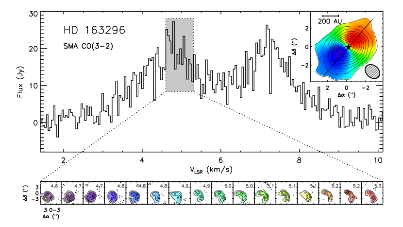
Figure 1.— CO(3-2) emission from the disk around HD 163296 observed with the SMA at a spectral resolution of 44 m s^-1. Top plot shows the line profile, summed within a 6 arcsec box using the MIRIAD task imspec (neglecting emission with absolute values between $\pm$2$\sigma$). Channel maps across the bottom show the segment of the line indicated by the shaded gray box at its full spatial and spectral resolution, imaged with a 1$\farcs$0 taper to bring out the large-scale emission (complete channel maps are provided in Appendix A). LSR velocity is indicated by the numbers in the upper right of each channel. Contours are [3,6,9,…]$\times$0.55 Jy beam^-1 (the rms noise). Inset in the upper right corner is a zeroth (contours) and first (colors) moment map of the CO(3-2) line emission. The 2$\farcs$0$\times$1$\farcs$7 beam is indicated in the lower right of the inset. Note that while the colors in the channel and moment maps both represent LSR velocity (blue is low; red is high), the scales are different for the two representations: the moment map contains the full line data, while the channel maps span only a subset of the line.

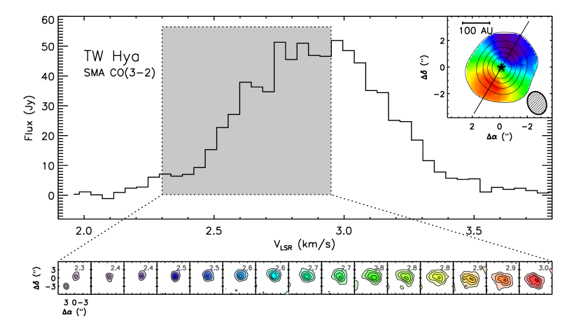
Figure 2.— Same as Figure 1 but for TW Hya. The channel maps were imaged with a 1$\farcs$2 Gaussian taper to emphasize the emission on larger scales, and the contours are [4,8,12,…]$\times$0.55 Jy beam^-1 (the rms noise). For the full set of channel maps, see Appendix A.

4. Analysis

In order to constrain the turbulent linewidth in the disks around TW Hya and HD 163296, we fit models of the temperature, density, and velocity structure to the high spectral resolution CO(3-2) line data. For the initial modeling effort presented here, we use two well-tested physical models of disk structure: (1) power-law models of the disk temperature structure combined with tapered surface density profiles corresponding to the functional form predicted for a simple viscous accretion disk (Lynden-Bell & Pringle, 1974; Hartmann et al., 1998), and (2) the 1+1D radiative transfer models developed by D’Alessio et al. to reproduce the dust emission represented in the SEDs of young systems. These models are described in more detail in Section 4.1.

We use these two classes of models because they are well established and have been successful in describing the observed structure of circumstellar disks across a wide range of wavelengths, particularly in the submillimeter (see, e.g., Calvet et al., 2002, 2005; Andrews et al., 2009). However, each class of models has limitations. The similarity solution models have a large number of free parameters, some with significant degeneracies (see discussion in Andrews et al., 2009). By fitting only the CO(3-2) emission, these models also neglect potential information provided by dust emission, including stronger constraints on the disk density. However, the neglect of dust emission avoids complications due to heating processes and chemistry that affect gas differently than dust. The D’Alessio et al. models of dust emission include only stellar irradiation and viscous dissipation as heating sources, and do not take into account the additional heating processes that may affect molecular line strengths in the upper layers of circumstellar disks (Qi et al., 2006). While the constraints from the dust continuum reduce the number of free parameters in this class of models, they also have the disadvantage of an unrealistic treatment of the density structure at the disk outer edge: since they are simply truncated at a particular outer radius, they are not capable of simultaneously reproducing the extent of gas and dust emission in these systems (Hughes et al., 2008). The similarity solution models are vertically isothermal, which is an unrealistic assumption. With only one molecular line included in the model, this limitation will not affect the results of the study presented here, although caution should be exercised when applying the best-fit model parameters to other lines.

The primary reason for using the two types of models, however, is that they differ substantially in their treatment of the disk temperature structures. For the D’Alessio et al. models, the temperature structure is fixed by the dust continuum. The similarity solution models, by contrast, allow the temperature to vary to best match the data. There are a few independent constraints on temperature: it should increase with height above the midplane, due to surface heating by the star and low viscous heating in the midplane, and the dust will generally not be hotter than the gas, since the gas is subject to additional heating processes beyond the stellar irradiation that determines dust temperature. The temperature structure in the disk is the single factor most closely tied to the derived value of the turbulent linewidth (see discussion in Section 4.4), which will be model-dependent. We therefore fit both classes of models to the data, in order to compare the model-dependent conclusions about turbulent linewidth for two distinct types of models with very different treatments of gas temperature. The spatial dynamic range of the data is insufficient to investigate radial variations in turbulent linewidth. We therefore assume a global value, $\xi$, that will apply to size scales commensurate with the spatial resolution of the data.

4.1. Description of Models

4.1.1 D’Alessio et al. Models

The D’Alessio et al. models are described in detail in D’Alessio et al. (1998, 1999, 2001, 2006). Here we provide a general outline of the model properties and discuss the particular models used in this paper.

The D’Alessio et al. models were developed to reproduce the unresolved SEDs arising from warm dust orbiting young stars, although they have also been demonstrated to be successful at reproducing spatially resolved dust continuum emission at millimeter wavelengths (see, e.g., Calvet et al., 2002; Hughes et al., 2007, 2009a) as well as spatially-resolved molecular line emission (see, e.g., Qi et al., 2004, 2006). The models include heating from the central star and viscous dissipation within the disk, although they tend to be dominated by stellar irradiation. The structure is solved iteratively to provide consistency between the irradiation heating and the vertical structure. The mass accretion rate is assumed to be constant throughout the disk. The assumed dust properties are described by Calvet et al. (2002), and the model includes provisions for changing dust properties, dust growth, and settling. We allow the outer radius of the model to vary to best reproduce the extent of the molecular line observations.

We use the structure model for TW Hya that was developed by Calvet et al. (2002) and successfully compared to molecular line emission by Qi et al. (2004, 2006). For HD 163296, we use a comparable model that reproduces the spatially unresolved SED and is designed to reproduce the integrated line strengths of several CO transitions as well as other molecules (Qi et al., in prep).

Since the D’Alessio et al. models were developed primarily to reproduce the dust emission from the SED, we are required to fit several parameters to match the observed CO(3-2) emission using the SED-based models. We fit the structural parameters {$R_{D}$, $X_{\mathrm{CO}}$} (the disk outer radius and CO abundance, respectively), the geometrical parameters {$i$, PA} (the disk inclination and position angle), and the turbulent linewidth, {$\xi$}.

4.1.2 Viscous Disk Similarity Solutions

We also fit the observations using a power-law temperature distribution and surface density profile that follows the class of similarity solutions for evolving viscous accretion disks described by Lynden-Bell & Pringle (1974) and Hartmann et al. (1998). This particular method of parameterizing circumstellar disk structure has a long history of success in reproducing observational diagnostics, although with limitations. Theoretical predictions of the power-law dependence of temperature for accretion disks around young stars were first made by Adams & Shu (1986), and power-law parameterizations of temperature and surface density have been used by many studies since then (e.g. Beckwith et al., 1990; Beckwith & Sargent, 1991; Mundy et al., 1993; Dutrey et al., 1994; Lay et al., 1994; Andrews & Williams, 2007). The similarity solutions are equivalent to a power-law surface density description in the inner disk, but with an exponentially tapered outer edge, which was shown by Hughes et al. (2008) to better reproduce the extent of gas and dust emission than traditional power-law descriptions with abruptly truncated outer edges. Recent high spatial resolution studies have used this class of models to reproduce successfully the extent of gas and dust emission in circumstellar disks from several nearby star-forming regions (e.g. Andrews et al., 2009; Isella et al., 2009).

The temperatures and surface densities of these models are parameterized as follows:

$$T(R)=T_{100}\left(\frac{R}{100\mathrm{AU}}\right)^{-q}$$ (1)

$$\Sigma(R)=\frac{c_{1}}{R^{\gamma}}\exp{\left[-\left(\frac{R}{R_{c}}\right)^{2-\gamma}\right]}$$ (2)

where $R$ is the radial distance from the star in AU, $T_{100}$ is the temperature indicated by the CO(3-2) line at 100 AU from the star, $q$ describes how the temperature decreases with distance from the star, $c_{1}$ is a constant describing the surface density normalization, $R_{c}$ is a constant related to the radial scale on which the exponential taper decreases the disk density, and $\gamma$ describes how surface density falls with radius in the inner disk regions (comparable to the parameter $p$ in typical power-law descriptions of surface density; see e.g. Dutrey et al., 1994, for a description of the power-law model parameters). Because the high optical depth of the CO(3-2) line is a poor tracer of the radial dependence of $\Sigma$, we fix $\gamma$ at a value of 1 for both systems, which is consistent with theoretical predictions for a constant-$\alpha$ accretion disk (Hartmann et al., 1998), as well as observations of young disks in Ophiuchus (Andrews et al., 2009) and previous studies of the continuum emission from these systems (Hughes et al., 2008). We therefore fit the high spectral resolution CO(3-2) observations using four structural parameters, {$T_{100}$, $q$, $c_{1}$, $R_{c}$}, two geometric parameters, {$i$, PA}, and the turbulent linewidth, {$\xi$}.

4.2. Modeling Procedure

We assume that the disks have a Keplerian velocity field, using stellar masses and distances from the literature to model the rotation pattern (0.6 M_☉ at 51 pc for TW Hya and 2.3 M_☉ at 122 pc for HD 163296; see Calvet et al., 2002; Webb et al., 1999; Mamajek, 2005; van den Ancker et al., 1998). Gas and dust are assumed to be well-mixed in both models; the gas-to-dust mass ratio is fixed at 100 while the CO abundance is allowed to vary in the D’Alessio et al. models in order to reproduce the CO emission while maintaining consistency with the dust continuum emission from which the model was derived. Since we don’t include continuum emission in the fits, we fix the CO abundance at $10^{-4}$ for the similarity solution models because there is no constraint on the relative content of gas and dust. In regions of the disk where the temperature drops below 20 K, the CO abundance is reduced by a factor of $10^{4}$ to simulate the effects of freeze-out onto dust grains. We assume a global, spatially uniform value of the turbulent linewidth, which is implemented as an addition to the thermal linewidth.

In order to compare the models with the data, the systemic velocity, or central velocity of the line, must be determined. We calculated the visibility phases for the spatially integrated CO(3-2) emission and fit a line to the central few channels (45 for HD 163296; 12 for TW Hya) to determine the systemic velocity. Figure 3 presents a cartoon of this method, which is largely model-independent, requiring only the assumption that the flux distribution is axisymmetric. The visibility phases encode information about the spatial symmetry of the line emission in each channel: for a Keplerian disk, it is most symmetric, and therefore the phase is zero, at line center. The channel maps are most asymmetric about disk center near the line peaks, with opposite spatial offsets at the two line peaks. The phase therefore reverses sign between one peak and the other, with an approximately linear relationship near the line center. The linear fit therefore uses the integrated emission from the central few channels to pinpoint the precise location where the phase is zero and the line is most symmetric, i.e., at the systemic velocity (it should be noted that if there were large-scale asymmetries in the CO data this method would not produce a reliable systemic velocity, but we see no evidence of such asymmetries in the data). We derive a systemic velocity of 5.79 km s^-1 for HD 163296 and 2.86 km s^-1 for TW Hya. In order to generate model emission with the appropriate velocity offset, we create a model image at higher spectral resolution than the data, and then re-bin it at the appropriate velocity sampling using the MIRIAD task regrid.

Figure 3.— Cartoon showing the amplitude and phase of a spectral line as a function of velocity and how they correspond to the spatial distribution of flux in the disk. The line wings originate from small areas of fast-moving material close to the star, resulting in low amplitude and small phase offsets. The line peaks arise from a large surface area of intermediate-velocity material with a large spatial offset from the star, resulting in high amplitudes and large visibility phases. The line center is symmetric and therefore has zero phase. We determined the systemic velocity by assuming an axisymmetric flux distribution and fitting a line to the central channels of the visibility phases (similar to the dotted line in the figure). The systemic velocity is the point at which the asymmetry changes sign and the line crosses zero.

Each disk model specifies a particular density, temperature, and velocity structure. We use the Monte-Carlo radiative transfer code RATRAN (Hogerheijde & van der Tak, 2000) to calculate equilibrium populations for each rotational level of the CO molecule and generate a sky-projected image of the CO(3-2) line emission at a given viewing geometry {$i$,PA} for each model. We compare these simulated models directly to the data in the Fourier domain. In order to sample the model images at the appropriate spatial frequencies for comparison with the SMA data, we use the MIRIAD task uvmodel. We then compute the $\chi^{2}$ statistic for each model compared with the data using the real and imaginary simulated visibilities. Due to the high computational intensity of the molecular line radiative transfer, it is prohibitively time-intensive to generate very large and well-sampled grids of models for the $\chi^{2}$ comparison. Instead, we move from coarsely-sampled grids that cover large regions of parameter space to progressively more refined (but still small) grids to avoid landing at a local minimum. However, this has the result that the degeneracies of the parameter space are poorly characterized. A discussion of these degeneracies is included in Section 4.4 below.

4.3. Best-fit Models

The best-fit parameters for both types of models are presented in Table 2. Their temperature and density structures are plotted in Figure 6. Note that the midplane temperatures for the similarity solution models are likely much lower than indicated; the power-law temperature representation parameterizes only the radial dependence of temperature in the upper disk layers from which the optically thick CO(3-2) emission arises.

The $\chi^{2}$ values for the similarity solutions are lower than for the D’Alessio et al. models; this may be due to gradients between gas and dust properties that influence the D’Alessio et al. model fit but not the similarity solution models. A sample of channel maps comparing the data with the two classes of models are presented in Figures 4 and 5. From the residuals in the D’Alessio et al. model of TW Hya, there is evidence of a mismatch in the temperature gradient between the model and the data: the residuals are systematically more positive near the disk center and negative farther from the star. For HD 163296, the difference is more subtle: the residuals are small and apparently spatially random (with the exception of some positive emission seen near a velocity of 4.7 m s^-1 but not near the corresponding position in the mirror half of the line). It should be noted that the CO abundance derived for this source is extremely low, nearly three orders of magnitude below the standard value of $10^{-4}$. The reason for this is most likely an overestimate of the temperature in the upper disk layers. In the absence of better information, this SED model was created with a very low turbulent linewidth ($\sim$50 m s^-1) and correspondingly little stirring of large dust grains above the midplane. The addition of a turbulent linewidth comparable to the best-fit value for the CO lines would substantially reduce settling and lower the temperature of the upper disk layers as more of the mass is placed in large dust grains. Such a model is under development by Qi et al. (in prep), and can also aid in explaining the spatial distribution of multiple CO transitions and CO isotopologue emission from this disk.

One important outcome of the modeling process is the consistency in the measurement of turbulent linewidth in each source for the two types of models, despite the differences in their treatment of temperature. In both types of models for HD 163296, the best-fit model with turbulence fits the data better than a comparable model without turbulence at the $\sim 3\sigma$ level. If the turbulent linewidth is fixed at 0 m s^-1 in the similarity solution and the temperature allowed to vary to compensate, the parameter $T_{100}$ must increase to 77 K; even then, the $\chi^{2}$ for a model with higher temperature and no turbulence is a poorer fit than the best-fit model with turbulence at the $\sim 3\sigma$ level (the line profile for this model is plotted in Figure 4). The TW Hya data are consistent with no turbulent linewidth whatsoever.

Table 2Best-Fit Model Parameters

Parameter	HD 163296	TW Hya
Similarity Solution
$T_{100}$ (K)	60	40
$q$	0.5	0.4
$c_{1}$ (cm-2)	$1.0\times 10^{12}$	$1.0\times 10^{11}$
$R_{c}$ (AU)	150	50
$\xi$ (m s-1)	300	$\lesssim 40$
$i$ (∘)	40	6.0
PA (∘)	131	155
Reduced $\chi^{2}$	2.642	2.106
D’Alessio et al. Model
$R_{D}$ (AU)	525	155
$X_{\mathrm{CO}}$	$5\times 10^{-7}$	$1.5\times 10^{-5}$
$\xi$ (m s-1)	300	$\lesssim 40$
$i$ (∘)	40	5
PA (∘)	138	155
Reduced $\chi^{2}$	2.885	2.108

Figure 4.— Comparison of CO(3-2) emission from HD 163296 between the data and best-fit models for a subset of the data. The top row shows the same subset of channels as in Figure 1. The central set of channel maps shows the corresponding channels of the best-fit similarity solution model and the residuals (subtracted in the visibility domain). The bottom set of channel maps shows the best-fit D’Alessio et al. model and residuals. Contour levels, beam sizes, and imaging parameters are identical to those in Figure 1. An additional line profile for the best-fit similarity solution without turbulence is overplotted in gray.

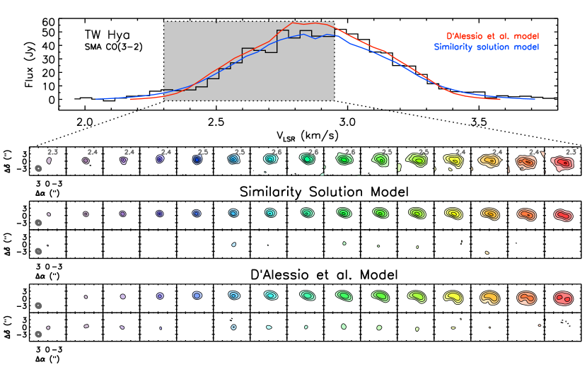
Figure 5.— Same as Figure 4 but for TW Hya. The channels, contour levels, and imaging parameters are identical to those in Figure 2.

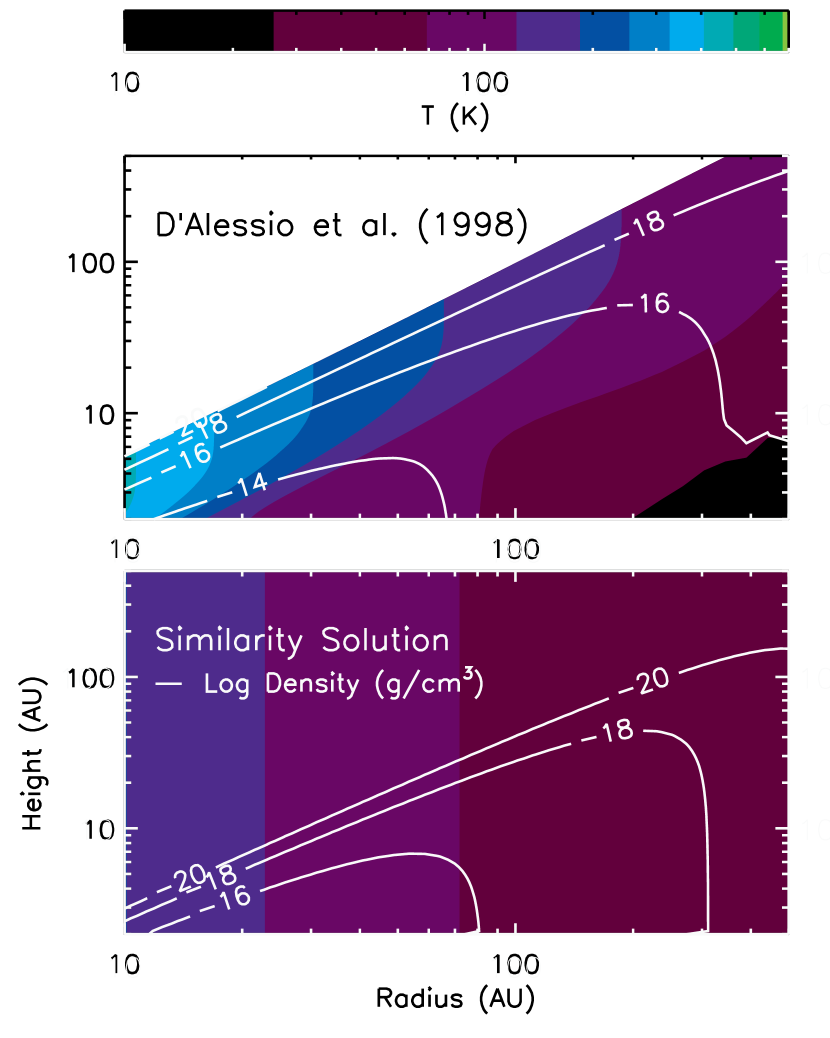
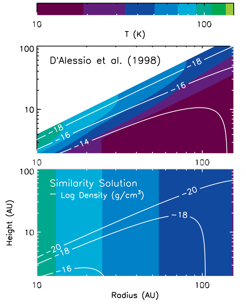
Figure 6.— Comparison between the temperature and density structures of the similarity solution and D’Alessio et al. models for HD 163296 (left) and TW Hya (right). The bar across the top shows the temperature scale represented by the colors, while the white contours represent density, marked with the base 10 logarithm of the total (gas+dust) mass density in units of g cm^-3. Note that while the D’Alessio et al. model of HD 163296 appears to be two orders of magnitude more dense than the similarity solution model, the CO abundance is more than two orders of magnitude lower, making the CO mass densities comparable. The CO abundance of the TW Hya model is one order of magnitude lower than for the similarity solution. The abscissae of the plots are scaled to match the radial extent of the power-law disk model (excising the central 10 AU, which are not accessible with the data), although the similarity solution models will extend farther.

4.4. Parameter Degeneracies

In order to better characterize our ability to measure turbulent linewidth, it is important to understand its relationship to the other parameters. The interdependence between parameters other than the turbulent linewidth has been explored at length in previous papers (see, e.g., discussion of similarity solution parameters in Andrews et al., 2009), so here we focus on the relationships and degeneracies specific to the turbulent linewidth. There are four main categories of line broadening in circumstellar disks that are relevant to our investigation: rotational, thermal, turbulent, and optical depth. These types of line broadening are all incorporated in detail into the ray-tracing portion of the RATRAN radiative transfer code, and will be handled appropriately for a given disk structure. The goal is to understand how to distinguish the distinct contributions of each of these different sources of line broadening and their relationships to the parameters of our disk structure models.

As discussed above, a detailed characterization of the multi-dimensional parameter space is prohibitively computationally expensive. We therefore investigate parameter relationships by letting the two-dimensional $\chi^{2}$ values generated in Section 4.2 guide an investigation using a toy model of an optically thick spectral line profile to highlight the distinct contribution of each related parameter to the observable properties.

The $\chi^{2}$ values indicate that for the similarity solution models, the parameters that are most strongly degenerate with the turbulent linewidth are the temperature ($T_{100}$ and $q$) and inclination ($i$). This is unsurprising, given the obvious relationship between temperature and thermal broadening and between inclination and rotational broadening. The optically thick CO(3-2) line responds only weakly to variations in density, and the outer radius and position angle of emission should intuitively be unrelated to line broadening, hence the independence of turbulent linewidth from $c_{1}$, $R_{c}$, and PA. For the D’Alessio et al. models, inclination and CO abundance ($i$ and $X_{CO}$) have the strongest relationships with turbulent linewidth. The contribution of the CO abundance in this case can be understood as a thermal broadening effect: because of the vertical temperature gradient (see Figure 6), the CO abundance controls the location of the $\tau$=1 surface and therefore the apparent temperature of the CO(3-2) line emission.

To characterize the effects of these variables on the observable properties of the CO(3-2) emission, we investigate their influence on a toy model of optically thick line emission. We assume a power-law temperature distribution for a geometrically flat, optically thick, azimuthally symmetric circumstellar disk. In the Rayleigh-Jeans approximation, the brightness of the line at a given frequency will be directly proportional to the temperature. We include two sources of line broadening, thermal and turbulent, implemented by the relationship $\Delta v(r)=\sqrt{2k_{B}T(r)/m+\xi^{2}}$, where $\Delta v$ is the total linewidth, $\xi$ is the turbulent linewidth, and the thermal linewidth is $\sqrt{2k_{B}T/m}$ where $k_{B}$ is Boltzmann’s constant, $T$ is the local temperature in the disk, and $m$ is the average mass per particle. Rotational broadening is implicitly included in the assumed Keplerian rotation pattern of the material, so that in polar coordinates, the central frequency of the line as a function of position is given by $\nu(r,\theta)=\nu_{0}/c\sqrt{GM_{*}/r}\sin{i}\cos{\theta}$, where $\nu_{0}$ is the line frequency and $M_{*}$ is the stellar mass. The line profile at any point in the disk is then given by

$$\phi(\nu,r)\propto\frac{T(r)}{\Delta v(r)\nu_{0}/c}\exp\left[\frac{-(\nu-\nu_{0})^{2}}{(\Delta v(r)\nu_{0}/c)^{2}}\right]$$ (3)

where $\nu_{0}$ is the frequency of the line center and $c$ is the speed of light. We project the disk onto the sky according to its inclination, and integrate over the $r$ and $\theta$ coordinates across the extent of the elliptical disk to calculate the line profile as a function of frequency. We investigate the contribution of the different sources of broadening by varying $\xi$, $T(r)$, and $i$ to correspond to the turbulent, thermal, and rotational broadening effects. Here we discuss the ways in which turbulent broadening can be distinguished from the other two effects in the context of our toy model.

Temperature — The left panel of Figure 7 shows model line profiles that illustrate the relationship between broadening due to temperature and broadening due to a global turbulent linewidth. The solid line is the model line profile calculated using values from the best-fit similarity solution: $T_{100}$=60 K, $q$=0.5, and $\xi$=300 m s^-1. The dotted line represents the profile for a model with the same parameters but no turbulent linewidth. To create the dashed line profile, the temperature was varied until the peak line flux of the model without turbulence matched the peak flux of the original model with turbulence. This sequence of line profiles illustrates how thermal and turbulent broadening produce distinct effects on the observable properties of the data, rather than being fully interchangeable. Since increases in temperature increase the line flux throughout the disk while turbulence simply redistributes the flux in frequency space, turbulence tends to shift flux from the line peaks to the center, changing the shape of the line. As a result, the peak-to-center line flux ratios will be different for line profiles with comparable widths and peak fluxes, depending on the relative contributions of turbulence and temperature to line broadening. The difference between the best-fit 300 m s^-1 turbulent linewidth in HD 163296 and a comparable model without turbulence corresponds to a 30% change in peak-to-center line flux in the context of this toy model, which should be easily distinguishable given the quality of our data.

As mentioned above, the temperature power law index $q$ is also found to be degenerate with the turbulent linewidth. The effects of this parameter are similar to those of the temperature normalization, illustrated in the left panel of Figure 7: varying $q$ also alters the peak-to-center ratio of the line. However, since the emission from both the peaks and the center is dominated by spatial scales of order 100 AU, the relevant spatial dynamic range is not large enough for variations of $q$ (within the uncertainties) to account for broadening on the scale of the derived turbulent linewidth.

Inclination — The right panel of Figure 7 shows model line profiles that illustrate the relationship between turbulent broadening and rotational broadening due to inclination. As in the left panel, we first generate a model with no turbulent broadening (dotted line), and then adjust the inclination until the peak flux matches the original line model (dashed line). In this case, the absence of turbulence once again alters the peak-to-center line ratio. But another obvious difference between the turbulent model and the more inclined model without turbulence is that rotational broadening through inclination alters the separation between the line peaks in velocity space. The sequence of toy models shows that the contribution of the 300 m s^-1 turbulent linewidth in the HD 163296 model corresponds to a 6^∘ change in inclination, in addition to the large depression of flux at the line center. Since spatially resolved spectra of the Keplerian rotation patterns in molecular lines allow for very precise determination of circumstellar disk inclination (to within a degree or less, given the stellar mass and assuming axisymmetry; see discussion in Qi et al., 2004), turbulent line broadening at the level detected in HD 163296 should be distinguishable from rotational broadening. It should be noted that rotational broadening includes the combined effects of inclination and stellar mass since the two variables are almost precisely degenerate to within $\sim$10^∘ (or tens of percent in mass): we cannot disentangle their effects. Nevertheless, since we allow inclination to vary for the assumed stellar mass, and have demonstrated that inclination can be distinguished from turbulent broadening in the toy model line profiles, the uncertainty in stellar mass will not strongly affect our determination of the turbulent linewidth.

We have focused this discussion on HD 163296 to investigate the robustness of the turbulent linewidth measurement rather than the upper limit for TW Hya. The situation is somewhat different for TW Hya, since the face-on disk orientation does not result in splitting of the line profile, so diagnostics like peak-to-trough ratios and peak separations do not apply. Nevertheless, the Keplerian rotation pattern – the combination of inclination and stellar mass – is still very precisely determined from the channel maps (Qi et al., 2004), and the temperature is well constrained by the brightness of the optically thick line. As a result, we achieve a strong constraint on the turbulent linewidth for this system. It should be noted that a turbulent linewidth comparable to that derived for HD 163296 would have a dramatic effect on the line profile for this system, since a 300 m/s turbulent linewidth would represent roughly a 50% perturbation on the observed 700 m/s FWHM of the CO(3-2) line.

Figure 7.— Model spectral line profiles for a geometrically flat, optically thick, azimuthally symmetric circumstellar disk (for details, see toy model description in Section 4.4). The left panel explores the relationship between thermal and turbulent line broadening, while the right panel explores the relationship between turbulent broadening and rotational broadening through changes in inclination. The solid line in each panel is generated using values from the best-fit similarity solution model ($T_{100}$=60 K, $q$=0.5, and $\xi$=300 m s^-1), while the dotted lines are the same model without turbulence, and the dashed lines seek to compensate for the lack of turbulence through the alternative line broadening mechanisms, scaled so that the peak flux is the same as the original model. The parameters for each line are given in the legend. The obvious differences between the solid and dashed lines in each panel (e.g., peak-to-center flux ratios and velocity separation between peaks) illustrate how the effects of rotational and thermal broadening differ from those of turbulent broadening in the context of this toy model.

5. Discussion

5.1. Comparison with Theory

The problem of accurately modeling and predicting the magnitude of velocity fluctuations arising from magnetohydrodynamic (MHD) turbulence has proven somewhat intractable, but a few general features seem to be agreed upon. The difficulty hinges largely on derived values of the parameter $\alpha$ and how they relate to the expected magnitude of the turbulent linewidth. The dimensionless parameter $\alpha$ was defined by Shakura & Sunyaev (1973) to describe the effective viscosity in terms of a proportionality constant multiplied by the largest velocity and length scales on which turbulence may act: the scale height and the sound speed. In mathematical terms, $\nu_{\mathrm{eff}}=\alpha c_{s}H$, where $\nu_{\mathrm{eff}}$ is the effective viscosity, $c_{s}$ is the sound speed, $H$ is the local scale height, and $\alpha$ is then an efficiency factor with a value $\leq$1. The magnitude of turbulent velocity fluctuations depends both on the value of $\alpha$ and on how this efficiency factor is apportioned between the sound speed and the scale height. If, for example, the majority of the power in turbulent fluctuations occurs at the length of the scale height, the velocity fluctuations can be as small as $\alpha c_{s}$ (perhaps augmented by a geometric factor of a few). On the other hand, if the proportionality factor $\alpha$ applies evenly to the length and velocity scales in the problem, the turbulent fluctuations could be as large as $\sqrt{\alpha}c_{s}$ (again possibly modified by a geometric factor). Since there is no evidence of shocks that would point to sonic or supersonic turbulence in circumstellar disks, it is unlikely that the turbulent velocity fluctuations would be much larger than $\sqrt{\alpha}c_{s}$.

It is clear that shearing box simulations of MHD turbulence with zero net magnetic field flux do not give reliable values of the viscosity parameter $\alpha$ due to numerical dissipation, which results in values of $\alpha$ that depend on resolution (Pessah et al., 2007; Fromang & Papaloizou, 2007). This is mitigated by the use of more realistic simulation conditions including vertical stratification (e.g., Stone et al., 1996; Fleming & Stone, 2003; Davis et al., 2010; Flaig et al., 2010), but the resulting dependence of $\alpha$ and therefore turbulent velocity fluctuations on the magnitude of the magnetic field is troublesome, since magnetic field strengths and geometries in circumstellar disks are unconstrained by observations (e.g., Hughes et al., 2009b). The inclusion of vertical gravity has also been shown to lead to convergence (e.g. Davis et al., 2010; Flaig et al., 2010). It is perhaps instructive to investigate how $\alpha$ may be related to the observed turbulent linewidth in the context of shearing-box simulations. Quantities typically reported for shearing boxes include the shear stress $-B_{x}B_{y}/4\pi$, where $B_{x}$ and $B_{y}$ are the magnetic field along the $x$ and $y$ directions, respectively; Reynolds stress $\rho v_{x}\delta v_{y}$, where $\rho$ is density, $v_{x}$ is the $x$ component of velocity, and $\delta v_{y}$ is the $y$ component of velocity without shear; and the magnitude of velocity fluctuations along the different dimensions of the simulation $\rho v_{x,y,z}^{2}/2$. Each of these quantities is routinely normalized by the initial midplane pressure, $P_{0}$ (see, e.g., Stone et al., 1996; Davis et al., 2010). The total stress $T$ is then the sum of the Maxwell and Reynolds stresses, and is directly proportional to the viscosity parameter $\alpha$, according to the relationship $T=\alpha\rho c_{s}^{2}$, where $c_{s}$ is the sound speed. It is then straightforward to relate $\alpha$ to the turbulent velocity as a function of sound speed:

$$\alpha=\frac{T}{\rho v_{\mathrm{turb}}^{2}}\frac{v_{\mathrm{turb}}^{2}}{c_{s}^{2}}$$ (4)

$$\alpha=\frac{T/P_{0}}{2(\rho v_{z}^{2}\cos^{2}i+\rho v_{x,y}^{2}\sin^{2}i)/2P_{0}}\frac{v_{\mathrm{turb}}^{2}}{c_{s}^{2}}$$ (5)

where $v_{\mathrm{turb}}$ is the measured turbulent linewidth (typically the FWHM calculated from $\xi$, which is the $1/e$ half-width) and $i$ is the disk inclination. Using reported values of the relevant simulation parameters from Davis et al. (2010), $\alpha\sim 3(v_{\mathrm{turb}}/c_{s})^{2}$ for a face-on disk, and $\alpha\sim 1.5(v_{\mathrm{turb}}/c_{s})^{2}$ for an edge-on disk. For the value of $\alpha\sim 0.01$ derived in Davis et al. (2010), this predicts a midplane turbulent linewidth of roughly 6-8% of the sound speed, depending on the source geometry.

Observational attempts at constraining the value of $\alpha$ in circumstellar disks, while generally quite uncertain, seem to cluster near values of 10^-2, with large scatter (e.g., Hartmann et al., 1998; Andrews et al., 2009). If the velocity fluctuations are estimated as $\sqrt{\alpha}c_{s}$, this result would imply velocity fluctuations up to 10% of the sound speed near the midplane, although this global value is likely to vary widely depending on local conditions that affect the ionization fraction and the coupling of ions and neutrals. A theoretical comparison between circumstellar disks and the Taylor-Couette flow by Hersant et al. (2005) finds that the 100 m s^-1 turbulent linewidth (of order $\lesssim$30% of the sound speed) derived from low spectral resolution observations of DM Tau by Guilloteau & Dutrey (1998) are on par with expectations from laboratory measurements by Dubrulle et al. (2005). There is some evidence, both from the study of FU Ori objects (Hartmann et al., 2004) and global MHD simulations of stratified disks (e.g. Fromang & Nelson, 2006), that the turbulent linewidth may be larger at several scale heights above the midplane of the disk, perhaps up to 40% of the sound speed. While these estimates affect the local value of $\alpha$, it should also be noted that there are global disk features that may also affect the measured turbulent linewidth. In the dense inner disk, dead zones may form near the midplane where the ionization fraction is too low to support the MRI (e.g. Sano et al., 2000). However, these should not be relevant for our observations since the predicted extent of a dead zone in these disks is interior to a radius of 5-25 AU for TW Hya and 10-63 AU for HD 163296, depending on the assumed grain properties (N. Turner 2010, private communication); these size scales are significantly smaller than the linear scale probed by our observations.

In this context, HD 163296 seems to fit in fairly seamlessly, with a turbulent linewidth of 300 m s^-1 corresponding to about 40% of the sound speed at the size scales probed by our data (if 1$\farcs$5 corresponds to $\sim$180 AU at a distance of 122 pc). If the turbulent linewidth drops by a factor of a few between the upper layers probed by the CO(3-2) line and the midplane (as predicted by, e.g., Fromang & Nelson, 2006), this implies a turbulent linewidth of $\sim$0.1 $c_{s}$ near the midplane, consistent with $\alpha\sim 0.01$. The lower turbulent linewidth in TW Hya, $\lesssim$10% of the local sound speed at the scale of our observations (80 AU at 51 pc), could be associated with a lower global value of $\alpha$, although the reason for such a difference is unclear. Following Andrews et al. (2009), the best-fit similarity solution model parameters imply $\alpha$ = 0.03 for TW Hya and 0.009 for HD 163296, although these numbers are quite uncertain given the reliance on the optically thick CO(3-2) tracer for the determination of density. The D’Alessio et al. models use $\alpha$ = 0.0018 for TW Hya and 0.003 for HD 163296. Perhaps the only conclusion that should be drawn from this estimate is that our observations are consistent with estimates that place $\alpha$ in the range of $10^{-2}$-10^-3. With a sample of only two sources and with a wide range of theoretical results and approaches to the study of turbulence, it can be difficult to compare our results to theoretical predictions in a detailed way. Nevertheless, the detection of a turbulent linewidth in the HD 163296 system and the upper limit on turbulence in the TW Hya system are suggestive. There are several potential explanations for this difference rooted in theoretical studies of protoplanetary disk turbulence.

Inclination and Vertical Structure — In general, the CO(3-2) line emission from these systems is expected to be optically thick, and therefore will arise from the tenuous upper disk layers several scale heights above the midplane. However, this simple picture can be complicated by geometry and velocity: the combination of inclination and rotational line broadening in HD 163296 will permit the escape of radiation from deeper layers of the disk. As a result, a different vertical height may be probed in the HD 163296 system than in TW Hya. Naively, it would be expected that the turbulent linewidth in TW Hya should be larger as a result, since turbulence is predicted to become stronger farther from the midplane. It is difficult to calculate accurately the height above the midplane from which the CO(3-2) emission originates, both because it varies by position across the disk and velocity offset across the line, and because it depends on very poorly constrained quantities like the vertical gradients in gas temperature and density. Nevertheless, a rough estimate at line center for the D’Alessio et al. models places the origin of the emission at approximately 2 scale heights above the midplane for TW Hya and 3 for HD 163296 at the radii of 80 and 180 AU corresponding to the respective linear resolution of the observations for each source. This suggests that the difference in turbulent linewidth for the two sources could be due to the different physical regions probed by the line. But given the uncertainties, the height of formation is not constrained stringently enough to definitively demonstrate that this is the case. It is also possible that poor coupling of ions to neutrals in the low-density uppermost disk layers could inhibit the detection of turbulence even if it is present. This may also depend on the relative amounts of small dust grains in the upper layers of the two disks, since small grains are more adept at absorbing free electrons.

Stellar Mass and Ionizing Flux — One of the factors determining the extent of turbulent regions in circumstellar disks is the magnitude of ionizing X-ray flux from the star (e.g., Gammie, 1996; Igea & Glassgold, 1999). With stellar masses differing by a factor of 4, the radiation (and therefore ionization) properties of TW Hya and HD 163296 are likely to be quite different. Despite the tendency for X-ray flux to be lower for intermediate-mass than low-mass stars of comparable ages, HD 163296 has the largest X-ray flux of the sample of 13 Herbig Ae stars studied by Hubrig et al. (2009), comparable to that of lower-mass T Tauri stars. Nevertheless, its measured X-ray luminosity of $4.0\times 10^{29}$ erg s^-1 is still lower than that of TW Hya, which is estimated as $2.0\times 10^{30}$ erg s^-1 by Kastner et al. (1999). Given the comparable disk densities, by X-ray luminosity alone, TW Hya should be the more active disk. However, since we are observing these disks on relatively large spatial scales ($\sim$80 AU for TW Hya and $\sim$180 AU for HD 163296, with 1$\farcs$5 resolution viewed from their respective 51 and 122 pc distances), the ionization at these distances may instead be dominated by cosmic rays. It is extremely difficult to determine how the cosmic ray environment of these two sources might compare; if HD 163296 were located in a region of greater cosmic ray activity, that could account for the greater turbulent linewidth observed for this system.

Evolutionary State — One of the most obvious differences between TW Hya and HD 163296 is their respective evolutionary states. TW Hya is a 10 Myr-old transition disk with an inner cavity of $\sim$4 AU radius, while HD 163296 is a primordial disk with an inner radius consistent with the expected $\sim$0.4 AU extent of the dust destruction zone (see, e.g., Isella et al., 2007). It is possible that X-ray ionization and the MRI might operate differently at different stages of evolution; one example is the inside-out MRI clearing proposed by Chiang & Murray-Clay (2007) to explain the cavities in transition disks. In their scenario, the mass accretion rate onto the star can be explained entirely by the MRI operating on the disk inner rim, and requires no resupply from the outer disk; they therefore require little to no turbulent viscosity in the outer disk to explain the observed accretion rates in transitional systems. However, they note that their theory cannot be readily applied to primordial systems, leaving the viscous transport mechanism responsible for large accretion rates at earlier stages unexplained. There is no reason to expect MRI turbulence in the outer disk to “shut off” when a gap is opened, so while our observation of a small turbulent linewidth in the TW Hya system is consistent with the Chiang & Murray-Clay (2007) hypothesis, it is still surprising that the turbulent linewidth in HD 163296 should be so much larger. Another possibility unrelated to the MRI is that HD 163296 is still experiencing infall onto the disk from a remnant envelope. Since the high optical depth of the CO(3-2) line implies that most of the emission arises from the upper layers of the disk, such a scenario could mimic the signature of a turbulent linewidth that we observe; however, there is no observational evidence for an envelope in this system. We plan to address this possibility more thoroughly in a follow-up paper modeling multiple lines with lower optical depths that probe deeper towards the disk midplane.

5.2. Implications for Planet Formation

The presence of subsonic turbulence in protoplanetary accretion disks – likely substantially subsonic in the midplane – is consistent with the observations presented in this study. Subsonic turbulence has important implications for the formation and evolution of young planetary systems. One series of papers (Papaloizou & Nelson, 2003; Papaloizou et al., 2004; Nelson & Papaloizou, 2003, 2004) explores in detail the effects of turbulence on planet-forming disks. Their cylindrical models of turbulent disks have an average $\alpha$ in the range of $10^{-2}$-$10^{-3}$, but they demonstrate that the realistic implementation of turbulence results in different effects than are seen in laminar disk simulations with comparable values of $\alpha$ incorporated as an anomalous Navier-Stokes viscosity. They show that for massive planets, turbulence can widen and deepen the gap opened by massive protoplanets, and may reduce the accretion rate onto the protoplanet. For the case of migrating low-mass planet cores, the presence of turbulence in the disk can slow or even reverse the migration rate, converting the monotonic inward motion of the planet into a random walk. The presence of dead zones in the radial direction may also act to halt migration and encourage the survival and growth of protoplanets (e.g. Matsumura et al., 2009). Another important proposed effect of subsonic turbulence is to aid in concentrating planetesimals to allow them to collapse gravitationally (Johansen et al., 2007). MHD turbulence on these scales can also reduce the strength of the gravitational instability and reduce disk fragmentation (Fromang, 2005). There is also substantial literature on the effects of turbulence on dust settling and grain growth (e.g. Johansen & Klahr, 2005; Carballido et al., 2006; Ciesla, 2007; Balsara et al., 2009; Fromang & Nelson, 2009).

Although it is difficult to compare the properties of the simulations directly with our observations, the generic features of these models ($\alpha$=$10^{-2}$-$10^{-3}$, subsonic turbulence even in the upper disk layers) are globally consistent with the derived properties of turbulence in the disks around HD 163296 and TW Hya, indicating that these effects are likely to play a role in planet formation.

5.3. Future Directions

The most obvious improvement to our method would be to include additional spectral lines from different transitions or isotopologues of the CO molecule in order to provide independent constraints on the gas temperature. While this would necessarily introduce additional parameters into the model (i.e., to describe the vertical distribution of temperature and turbulence, as well as a consistent density distribution to properly account for the line opacity), the addition of several lines that are resolved in the spectral and spatial domains would more firmly constrain the models. It might also provide direct measurements of the vertical profile of the turbulent velocity structure. Dartois et al. (2003) and Panić et al. (2008) provide examples of studies that use multiple molecular lines to study the vertical structure of density and temperature in circumstellar disks; these techniques could be extended to constrain the turbulent linewidths in similar systems.

Another possibility is to observe ions rather than neutral species. This would eliminate complications introduced by the interaction between ions and neutrals, and would more directly probe the turbulent motions of the charged gas.

Even with the current set of observations, greater sensitivity would be extremely valuable in constraining the turbulent linewidth, since the distinctions between turbulent and thermal broadening are subtle (see Section 4.4). The vast improvements in sensitivity provided by the Atacama Large Millimeter Array will permit significantly better modeling of the velocity structure of young disks. Such data will also allow us to firmly rule out deviations from perfect Keplerian rotation that could complicate the derivation of turbulent linewidth. In addition, higher sensitivity combined with a greater spatial dynamic range will allow for the investigation of radial variations in the turbulent linewidth.

6. Summary and Conclusions

We have obtained the first spatially resolved observations of molecular line emission from two nearby circumstellar disks with spectral resolution finer than the expected turbulent linewidth. We fit these high spectral resolution observations of the CO(3-2) line emission using two well-tested models of circumstellar disk structure, and derive a turbulent linewidth of $\sim$300 m s^-1 for the disk around HD 163296 and $\lesssim$40 m s^-1 for the disk around TW Hya. The results are consistent for the two model classes despite their different treatments of the temperature structure of the disk, which is significant since thermal broadening is closely related to turbulent broadening. The magnitude of turbulent velocity fluctuations implied by these results – up to tens of percent of the sound speed – is broadly consistent with theoretical predictions for MRI turbulence in the upper layers of circumstellar disks, although it is unclear why the linewidth should be lower for TW Hya than for HD 163296.

These results demonstrate the potential of this method for constraining theories of the magnitude and spatial distribution of turbulence. Future observations with greater sensitivity, perhaps incorporating different molecular line species and isotopologues of the same molecule, have the potential to vastly improve our ability to characterize turbulence in these systems.

Appendix A Channel Maps

Figures 8 and 9 show the full channel maps for the high spectral resolution observations of the CO(3-2) emission from the disks around TW Hya and HD 163296. The line overlaid on the emission indicates the disk major axis. The TW Hya and HD 163296 maps have been imaged with Gaussian tapers of 1$\farcs$2 and 1$\farcs$0, respectively, to bring out the large-scale emission.

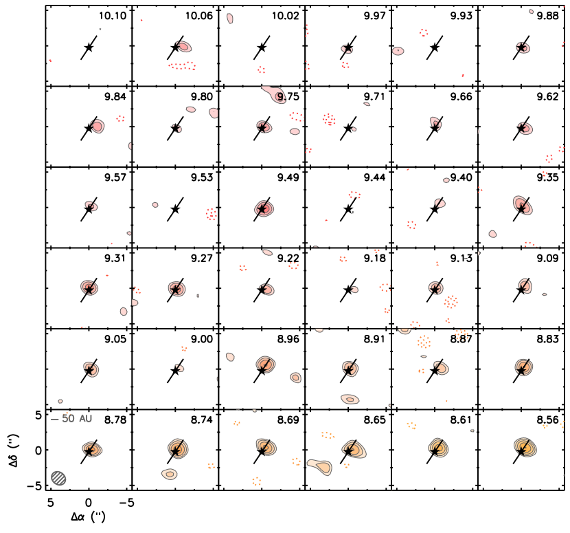
Figure 8.— Channel maps of the CO(3-2) line emission from the disk around HD 163296. The LSR velocity is indicated in the upper right of each channel, while the synthesized beam size and orientation (2$\farcs$0$\times$1$\farcs$7 at a position angle of 41^∘) is indicated in the lower left panel. The contour levels start at 2$\sigma$ and increase by factors of $\sqrt{2}$, where $\sigma$ is the rms noise of 0.6 Jy beam^-1. The star symbol indicates the disk center while the dark solid line indicates the disk position angle as determined by CO fitting in Section 4.

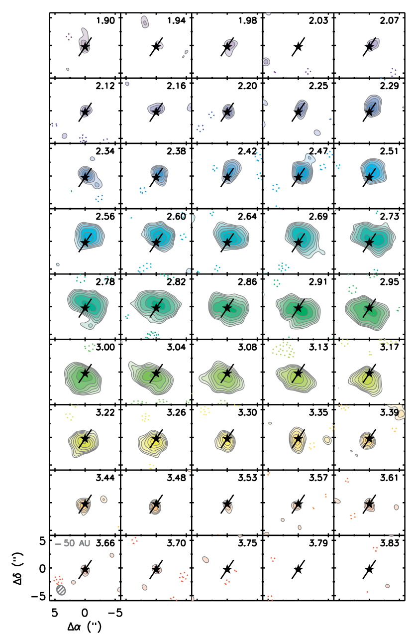
Figure 9.— Same as Figure 8 above, but for TW Hya. The beam size is 1$\farcs$9$\times$1$\farcs$4 at a position angle of 21^∘ and the contour levels are the same as in Figure 8.

References

- Adams & Shu (1986) Adams, F. C. & Shu, F. H. 1986, ApJ, 308, 836
- Andrews & Williams (2007) Andrews, S. M. & Williams, J. P. 2007, ApJ, 659, 705
- Andrews et al. (2009) Andrews, S. M., Wilner, D. J., Hughes, A. M., Qi, C., & Dullemond, C. P. 2009, ApJ, 700, 1502
- Balbus & Hawley (1991) Balbus, S. A. & Hawley, J. F. 1991, ApJ, 376, 214
- Balbus & Hawley (1998) —. 1998, Reviews of Modern Physics, 70, 1
- Balsara et al. (2009) Balsara, D. S., Tilley, D. A., Rettig, T., & Brittain, S. D. 2009, MNRAS, 397, 24
- Beckwith & Sargent (1991) Beckwith, S. V. W. & Sargent, A. I. 1991, ApJ, 381, 250
- Beckwith et al. (1990) Beckwith, S. V. W., Sargent, A. I., Chini, R. S., & Guesten, R. 1990, AJ, 99, 924
- Boss (2004) Boss, A. P. 2004, ApJ, 616, 1265
- Calvet et al. (2002) Calvet, N., D’Alessio, P., Hartmann, L., Wilner, D., Walsh, A., & Sitko, M. 2002, ApJ, 568, 1008
- Calvet et al. (2005) Calvet, N., D’Alessio, P., Watson, D. M., Franco-Hernández, R., Furlan, E., Green, J., Sutter, P. M., Forrest, W. J., Hartmann, L., Uchida, K. I., Keller, L. D., Sargent, B., Najita, J., Herter, T. L., Barry, D. J., & Hall, P. 2005, ApJ, 630, L185
- Carballido et al. (2006) Carballido, A., Fromang, S., & Papaloizou, J. 2006, MNRAS, 373, 1633
- Carr et al. (2004) Carr, J. S., Tokunaga, A. T., & Najita, J. 2004, ApJ, 603, 213
- Chiang & Murray-Clay (2007) Chiang, E. & Murray-Clay, R. 2007, Nature Physics, 3, 604
- Ciesla (2007) Ciesla, F. J. 2007, ApJ, 654, L159
- D’Alessio et al. (2001) D’Alessio, P., Calvet, N., & Hartmann, L. 2001, ApJ, 553, 321
- D’Alessio et al. (2006) D’Alessio, P., Calvet, N., Hartmann, L., Franco-Hernández, R., & Servín, H. 2006, ApJ, 638, 314
- D’Alessio et al. (1999) D’Alessio, P., Calvet, N., Hartmann, L., Lizano, S., & Cantó, J. 1999, ApJ, 527, 893
- D’Alessio et al. (1998) D’Alessio, P., Canto, J., Calvet, N., & Lizano, S. 1998, ApJ, 500, 411
- Dartois et al. (2003) Dartois, E., Dutrey, A., & Guilloteau, S. 2003, A&A, 399, 773
- Davis et al. (2010) Davis, S. W., Stone, J. M., & Pessah, M. E. 2010, ApJ, 713, 52
- Dent et al. (2005) Dent, W. R. F., Greaves, J. S., & Coulson, I. M. 2005, MNRAS, 359, 663
- Dubrulle et al. (2005) Dubrulle, B., Dauchot, O., Daviaud, F., Longaretti, P., Richard, D., & Zahn, J. 2005, Physics of Fluids, 17, 095103
- Dutrey et al. (1994) Dutrey, A., Guilloteau, S., & Simon, M. 1994, A&A, 286, 149
- Flaig et al. (2010) Flaig, M., Kley, W., & Kissmann, R. 2010, MNRAS, 1450
- Fleming & Stone (2003) Fleming, T. & Stone, J. M. 2003, ApJ, 585, 908
- Fromang (2005) Fromang, S. 2005, A&A, 441, 1
- Fromang & Nelson (2006) Fromang, S. & Nelson, R. P. 2006, A&A, 457, 343
- Fromang & Nelson (2009) —. 2009, A&A, 496, 597
- Fromang & Papaloizou (2007) Fromang, S. & Papaloizou, J. 2007, A&A, 476, 1113
- Gammie (1996) Gammie, C. F. 1996, ApJ, 457, 355
- Gammie & Johnson (2005) Gammie, C. F. & Johnson, B. M. 2005, in Astronomical Society of the Pacific Conference Series, Vol. 341, Chondrites and the Protoplanetary Disk, ed. A. N. Krot, E. R. D. Scott, & B. Reipurth, 145–+
- Grady et al. (2000) Grady, C. A., Devine, D., Woodgate, B., Kimble, R., Bruhweiler, F. C., Boggess, A., Linsky, J. L., Plait, P., Clampin, M., & Kalas, P. 2000, ApJ, 544, 895
- Guilloteau & Dutrey (1998) Guilloteau, S. & Dutrey, A. 1998, A&A, 339, 467
- Hartmann et al. (1998) Hartmann, L., Calvet, N., Gullbring, E., & D’Alessio, P. 1998, ApJ, 495, 385
- Hartmann et al. (2004) Hartmann, L., Hinkle, K., & Calvet, N. 2004, ApJ, 609, 906
- Hersant et al. (2005) Hersant, F., Dubrulle, B., & Huré, J. 2005, A&A, 429, 531
- Ho & Townes (1983) Ho, P. T. P. & Townes, C. H. 1983, ARA&A, 21, 239
- Hogerheijde & van der Tak (2000) Hogerheijde, M. R. & van der Tak, F. F. S. 2000, A&A, 362, 697
- Hubrig et al. (2009) Hubrig, S., Stelzer, B., Schöller, M., Grady, C., Schütz, O., Pogodin, M. A., Curé, M., Hamaguchi, K., & Yudin, R. V. 2009, A&A, 502, 283
- Hughes et al. (2007) Hughes, A. M., Wilner, D. J., Calvet, N., D’Alessio, P., Claussen, M. J., & Hogerheijde, M. R. 2007, ApJ, 664, 536
- Hughes et al. (2009a) Hughes, A. M., Wilner, D. J., Cho, J., Marrone, D. P., Lazarian, A., Andrews, S. M., & Rao, R. 2009a, ApJ, 704, 1204
- Hughes et al. (2009b) —. 2009b, ApJ, 704, 1204
- Hughes et al. (2008) Hughes, A. M., Wilner, D. J., Qi, C., & Hogerheijde, M. R. 2008, ApJ, 678, 1119
- Igea & Glassgold (1999) Igea, J. & Glassgold, A. E. 1999, ApJ, 518, 848
- Isella et al. (2009) Isella, A., Carpenter, J. M., & Sargent, A. I. 2009, ApJ, 701, 260
- Isella et al. (2007) Isella, A., Testi, L., Natta, A., Neri, R., Wilner, D., & Qi, C. 2007, A&A, 469, 213
- Johansen & Klahr (2005) Johansen, A. & Klahr, H. 2005, ApJ, 634, 1353
- Johansen et al. (2007) Johansen, A., Oishi, J. S., Low, M.-M. M., Klahr, H., Henning, T., & Youdin, A. 2007, Nature, 448, 1022
- Kastner et al. (1999) Kastner, J. H., Huenemoerder, D. P., Schulz, N. S., & Weintraub, D. A. 1999, ApJ, 525, 837
- Kastner et al. (1997) Kastner, J. H., Zuckerman, B., Weintraub, D. A., & Forveille, T. 1997, Science, 277, 67
- Lay et al. (1994) Lay, O. P., Carlstrom, J. E., Hills, R. E., & Phillips, T. G. 1994, ApJ, 434, L75
- Lynden-Bell & Pringle (1974) Lynden-Bell, D. & Pringle, J. E. 1974, MNRAS, 168, 603
- Mamajek (2005) Mamajek, E. E. 2005, ApJ, 634, 1385
- Matsumura et al. (2009) Matsumura, S., Pudritz, R. E., & Thommes, E. W. 2009, ApJ, 691, 1764
- Mundy et al. (1993) Mundy, L. G., McMullin, J. P., Grossman, A. W., & Sandell, G. 1993, Icarus, 106, 11
- Nelson & Papaloizou (2003) Nelson, R. P. & Papaloizou, J. C. B. 2003, MNRAS, 339, 993
- Nelson & Papaloizou (2004) —. 2004, MNRAS, 350, 849
- Panić et al. (2008) Panić, O., Hogerheijde, M. R., Wilner, D., & Qi, C. 2008, A&A, 491, 219
- Papaloizou & Nelson (2003) Papaloizou, J. C. B. & Nelson, R. P. 2003, MNRAS, 339, 983
- Papaloizou et al. (2004) Papaloizou, J. C. B., Nelson, R. P., & Snellgrove, M. D. 2004, MNRAS, 350, 829
- Pessah et al. (2007) Pessah, M. E., Chan, C., & Psaltis, D. 2007, ApJ, 668, L51
- Piétu et al. (2007) Piétu, V., Dutrey, A., & Guilloteau, S. 2007, A&A, 467, 163
- Qi et al. (2004) Qi, C., Ho, P. T. P., Wilner, D. J., Takakuwa, S., Hirano, N., Ohashi, N., Bourke, T. L., Zhang, Q., Blake, G. A., Hogerheijde, M., Saito, M., Choi, M., & Yang, J. 2004, ApJ, 616, L11
- Qi et al. (2008) Qi, C., Wilner, D. J., Aikawa, Y., Blake, G. A., & Hogerheijde, M. R. 2008, ApJ, 681, 1396
- Qi et al. (2006) Qi, C., Wilner, D. J., Calvet, N., Bourke, T. L., Blake, G. A., Hogerheijde, M. R., Ho, P. T. P., & Bergin, E. 2006, ApJ, 636, L157
- Ratzka et al. (2007) Ratzka, T., Leinert, C., Henning, T., Bouwman, J., Dullemond, C. P., & Jaffe, W. 2007, A&A, 471, 173
- Sano et al. (2000) Sano, T., Miyama, S. M., Umebayashi, T., & Nakano, T. 2000, ApJ, 543, 486
- Shakura & Sunyaev (1973) Shakura, N. I. & Sunyaev, R. A. 1973, A&A, 24, 337
- Stone et al. (1996) Stone, J. M., Hawley, J. F., Gammie, C. F., & Balbus, S. A. 1996, ApJ, 463, 656
- van den Ancker et al. (1998) van den Ancker, M. E., de Winter, D., & Tjin A Djie, H. R. E. 1998, A&A, 330, 145
- Webb et al. (1999) Webb, R. A., Zuckerman, B., Platais, I., Patience, J., White, R. J., Schwartz, M. J., & McCarthy, C. 1999, ApJ, 512, L63