The Three-Dimensional Structure of Cassiopeia A

Abstract

We used the Spitzer Space Telescope’s Infrared Spectrograph to map nearly the entire extent of Cassiopeia A between 5-40 µm. Using infrared and Chandra X-ray Doppler velocity measurements, along with the locations of optical ejecta beyond the forward shock, we constructed a 3-D model of the remnant. The structure of Cas A can be characterized into a spherical component, a tilted thick disk, and multiple ejecta jets/pistons and optical fast-moving knots all populating the thick disk plane. The Bright Ring in Cas A identifies the intersection between the thick plane/pistons and a roughly spherical reverse shock. The ejecta pistons indicate a radial velocity gradient in the explosion. Some ejecta pistons are bipolar with oppositely-directed flows about the expansion center while some ejecta pistons show no such symmetry. Some ejecta pistons appear to maintain the integrity of the nuclear burning layers while others appear to have punched through the outer layers. The ejecta pistons indicate a radial velocity gradient in the explosion. In 3-D, the Fe jet in the southeast occupies a “hole” in the Si-group emission and does not represent “overturning”, as previously thought. Although interaction with the circumstellar medium affects the detailed appearance of the remnant and may affect the visibility of the southeast Fe jet, the bulk of the symmetries and asymmetries in Cas A are intrinsic to the explosion.

1 Introduction

The three dimensional structure of core-collapse supernova explosions is of considerable interest, with implications for the explosion mechanisms (e.g. Akiyama et al., 2003; Wang, Baade & Patat, 2007), the role of rotation (e.g. Moiseenko, Bisnovatyi-Kogan & Gennady, 2007), pulsar “natal kicks” (e.g. Scheck et al., 2004) and for the subsequent interaction of ejecta with the circumstellar medium/pre-supernova wind (Schure et al., 2008). Asymmetries in the explosion and subsequent fallback have implications for mixing and the subsequent progression of explosive nucleosynthesis (Joggerst, Woosley & Heger, 2009). “Jet-induced” scenarios may play a role in forming supernova remnants such as Cassiopeia A (Cas A) (Wheeler, Maund, & Couch, 2008), and at their extreme, jet-dominated explosions may be responsible for gamma-ray bursts (e.g. Zhang, Woosley & Heger, 2004; Mazzali et al., 2005). There is plentiful evidence for asymmetric supernova explosions from structural and spectral data (Wang et al., 2002) and from spectropolarimetry (e.g. Wang et al., 2001; Tanaka et al., 2008).

Cas A provides a unique opportunity to study the three-dimensional supernova explosion structure because of the high velocities of its clumpy ejecta, seen both through Doppler and proper motions. It is the result of a core-collapse supernova approximately 330 years ago (Fesen et al., 2006) and is bright across the electromagnetic spectrum. The brightest emission in Cas A is concentrated onto the 200$\arcsec$ diameter Bright Ring where ejecta from the explosion are illuminated after crossing through and being compressed and heated by the reverse shock (Morse et al., 2004; Patnaude & Fesen, 2007). In a few locations, the position of the reverse shock itself has been identified just inside of the Bright Ring from the rapid turn-on of optical ejecta (Morse et al., 2004).

While most of the observed ejecta at all wavebands are concentrated on the Bright Ring, optical ejecta are also identified at and beyond the forward shock. The forward shock is visible as a thin ring of X-ray filaments approximately 300$\arcsec$ in diameter (Gotthelf et al., 2001). The canonical explanation for the far outer knots is that they are dense optical ejecta ($n_{e}\approx$4000–10,000 cm^-3; Fesen & Gunderson, 1996) which cool quickly ($t_{c}\approx$20–30 years; Kamper & van den Bergh, 1976) after passing through the reverse shock. They are reheated after they overtake the forward shock and encounter slow-moving ambient material which drives a slow shock into the supersonic dense ejecta and produces optical emission. In addition to the largely symmetric-appearing Bright Ring and forward shock, jets of Si- and S-rich ejecta extend out to large distances in the northeast and southwest with optical ejecta identified at a distance of $\approx 200\arcsec$ beyond the forward shock radius (Hwang et al., 2004). The jets may denote an axis of symmetry of the supernova explosion (e.g. Fesen et al., 2006). The optical knots are rapidly expanding with proper motions of 1000s of km s^-1 on the Bright Ring and up to 14,000 km s^-1 for the optical ejecta at the tip of the jets (Kamper & van den Bergh, 1976; Fesen et al., 2006). To the southeast, X-ray images show Fe-rich ejecta at a greater radius than Si-rich ejecta which has been interpreted as an overturning of ejecta layers during the supernova explosion (Hughes et al., 2000).

Large-scale Doppler mappings have been carried out at optical wavelengths primarily using S and O emission lines (Lawrence et al., 1995; Reed et al., 1995). These studies showed that the ejecta defining the Bright Ring outline a shell. Assuming that the shell is spherical, the Doppler velocities of ejecta knots can be converted into equivalent distances from the expansion center along the line of sight. The bulk of the ejecta are found to lie nearly in the plane of the sky and they are organized into distinct velocity structures such as the two complete rings - one blue shifted and one red shifted - that form the northern part of the Bright Ring.

A subsequent census of outlying optical ejecta showed that the northeast Jet is oriented within 6$\arcdeg$ of the plane of the sky with an opening angle of $\approx$25$\arcdeg$ (Fesen & Gunderson, 1996). The remainder of the outer optical knots are mostly located within $\pm 20\arcdeg$ of the plane of the sky and form a giant ring at the location of the forward shock (Fesen, 2001) although there are gaps in this distribution to the north and south (Fesen et al., 2006). None of the optical searches, either imaging or spectral, reveal fast-moving ejecta knots projected near the center of the remnant or a population of very-fast-moving outer optical knots projected onto the Bright Ring. One interpretation offered by Fesen (2001) for this “plane-of-the-sky” effect was that a near tangent viewing angle is required to detect ejecta knots. However, other effects may play a role in the lack of projected outer ejecta knots. For instance, imaging searches rely on large proper motions to detect outer ejecta knots and the filters used for the images may not have been broad enough to detect the highly red- or blue-shifted emission. While the spectral searches certainly had the wavelength range to detect fast-moving projected ejecta knots, the outer optical knots tend to be very faint unless they are encountering dense ambient media (Fesen, 2001; Fesen et al., 2006). Given the small amount of H$\alpha$ emission projected against Cas A (Fesen, 2001), any projected outer ejecta knots may be too faint to have been detected in the spectral searches. Therefore, despite the absence of a population of projected ejecta near the center of Cas A, either with velocities typical of outer ejecta or velocities typical of Bright Ring ejecta, the Bright Ring and the outer optical knot ring were believed to be limb-brightened shells (Lawrence et al., 1995; Fesen, 2001).

Spectra of the X-ray-emitting ejecta have also been mapped using a number of telescopes. The first mapping with the Einstein X-ray Observatory (Markert et al., 1983) and a subsequent mapping with ASCA (Holt et al., 1994) were at very low spatial resolution (1′-2′) and showed large-scale asymmetries in Doppler structure. These asymmetries were confirmed at higher spatial resolution with XMM-Newton (20″; Willingale et al., 2002, 2003) and the first 50-ks ACIS observation with the Chandra X-ray Observatory (4″; Hwang et al, 2001). At their improved spatial resolution, Willingale et al. (2002) found that the Si-rich ejecta forms the same general set of ring structures as the optical emission but the two distinct rings to the north are difficult to identify. The Fe-rich emission is concentrated in three main areas to the north, southeast, and west, but Willingale et al. (2003) determined that most of the Fe mass is concentrated within what they describe as a bipolar, double cone that is oriented at -55$\arcdeg$ from north and 50$\arcdeg$ out of the plane of the sky. Hughes et al. (2000) suggest an overturning in the explosion in the southeast, with the Fe emission extending out to the forward shock. Willingale et al. (2002) also found that in the north the centroid of the Fe-rich ejecta appears behind the Si-rich ejecta perhaps identifying another overturning region. A higher spatial resolution (1$\arcsec$) analysis using the Chandra ACIS 1 Ms data set plus two archival 50-ks data sets also shows the same optical ring structures in Si-rich emission and shows the strong Fe-K regions as dynamically distinct (Stage et al., 2004; Davis et al., 2005). A more recent analysis using Chandra High Energy Transmission Grating (HETG) spectra of the Si-He$\alpha$ triplet showed that, on 1$\arcsec$ spatial scales, the Si-rich ejecta has a great deal of substructure that is reminiscent of the variations seen in the optical data (Lazendic et al., 2006).

In this paper, we present a Doppler analysis of Cas A’s ejecta using infrared data from the Spitzer Space Telescope (Ennis et al., 2006) and X-ray data from the archival Chandra ACIS 1 Ms observation plus two other 50-ks observations (Stage et al., 2006; Davis et al., 2005). For the first time, we combine multiwavelength data into a full 3-dimensional reconstruction of Cas A. To this model, we add previously published X-ray results from Lazendic et al. (2006) and the jets and outer optical knots from Fesen (2001) and Fesen & Gunderson (1996). Based on this model, we draw conclusions about the multiple kinematic components and several major asymmetries in Cas A’s explosion.

2 Spitzer Observations and Data Analysis

The Spitzer Infrared Spectrograph (IRS) was used on 2005 January 13 to spectrally map nearly the full extent of Cas A with portions of the outer structures missing from some slits as shown in Figure 1. Low-resolution spectra (resolving power of $\sim$60-128) were taken between 5-15 µm (short-low module, SL) and 15-38 µm (long-low module, LL) with each module including two orders of wavelength. The long-wavelength (15-38 µm) spectra were taken in a single large map with 4$\times$91 pointings, using a single 6 s ramp at each position. To achieve the spatial coverage with the short-wavelength (5-15 µm) slit, a set of four quadrant maps were made, two with 4$\times$87 pointings and two with 3$\times$87 pointings, using a 6 s ramp at each position. The mapped area ranged from 6$\farcm$3$\times$5$\farcm$9 (SL) to 11$\farcm$0$\times$7$\farcm$8 (LL), with offsets between the maps produced in each of the two orders in each module of 3$\farcm$2 (LL) and 1$\farcm$3 (SL), along the slit direction. The effective overlap coverage of all modules and orders is 4$\farcm$9$\times$5$\farcm$8. The data used here were processed with the S12 version of the IRS pipeline, using the CUBISM package (Smith et al., 2007a) to reconstruct the spectra at each slit position, subtract the sky background, and create 3-dimensional data cubes as described in Smith et al. (2009). The statistical errors at each position in the data cube are calculated using standard error propagation of the BCD-level uncertainty estimates produced by the IRS pipeline.

2.1 The Bright Ring and Diffuse Interior Emission

There are a number of bright infrared ionic emission lines in Cas A from elements such as Ar, Ne, Si, S, Fe, and the 26 µm blend of Fe and O. For the most part, images made in these emission lines bear a close resemblance to optical images that primarily contain S and O emission (Ennis et al., 2006). In order to characterize the Bright Ring, we have chosen the 6.99 µm [Ar II] line and the 12.81 µm [Ne II] line. The [Ar II] line is relatively bright everywhere, even in Ne and O bright regions, and it is relatively isolated from other emission lines except for very weak 6.63 µm [Ni II] and possibly 6.72 µm [Fe II], although the latter transition is a⁴F${}_{9/2}-$a⁶D_7/2 which we expect to be negligible even given the [Fe II] detected in Cas A at other infrared wavelengths (Smith et al., 2009; Gerardy & Fesen, 2001; Rho et al., 2003). The [Ne II] line was used in order to calculate the [Ne II]/[Ar II] ratio, which varies considerably from place-to-place on the Bright Ring and may indicate inhomogeneous mixing between the oxygen-burning and carbon-burning layers of the progenitor star (Ennis et al., 2006; Smith et al., 2009). The disadvantage of the [Ar II] and [Ne II] lines is that the SL mapping did not extend out to the full extent of the Jet and Counterjet. The [Ar II] and [Ne II] images are shown in Figure 2.

In addition to the Bright Ring, there is Diffuse Interior Emission seen in the 10.51 µm [S IV] line, the 18.71 µm [S III] line, the 33.48 µm line of [S III], and the 34.82 µm line of [Si II] (Rho et al., 2008; Smith et al., 2009). Bright interior emission is seen at 26 µm as well. Since we detect no emission from any of the other infrared Fe lines (5.35 µm, 17.9 µm, etc) in the Diffuse Interior Emission, we believe that the 26 µm line is [O IV] with little or no contribution from [Fe II]. Support for this interpretation is provided by the high-resolution Spitzer spectra in Isensee et al. (2010). The [Si II] image, shown in Figure 2, shows both emission associated with the Bright Ring that is presumably shocked supernova ejecta, as well as emission in the interior. The Diffuse Interior Emission bears a striking resemblance to the free-free absorption observed at 74 MHz (Kassim et al., 1995). That absorption is thought to occur due to cold, photoionized ejecta that have not yet crossed the reverse shock (e.g. Hamilton & Fesen, 1998). We discuss the physical conditions in the unshocked ejecta more fully in §4.7.

This Diffuse Interior Emission is brightest and covers most of the remnant in the [O IV] and in the long wavelength [S III] and [Si II] lines. We have chosen to use both the 33.48 µm [S III] line and the 34.82 µm [Si II] line to map the interior emission. These lines are not entirely free of contamination from nearby lines – there is a small probability of [Fe III] at 33.04 µm and a reasonable probability of [Fe II] at 35.35 µm. However, these potentially contaminating lines lie on opposite sides of the [S III] and [Si II] lines, making it easier to detect their presence. The [O IV] line is less suitable for mapping the remnant because, although [O IV] dominates in the interior, on the Bright Ring there is the possibility of contamination from [Fe II] emission.

2.2 Preview of Velocity Structure: The First Moment Map

Figure 3 shows the 1st moment map of the [Ar II] line, calculated over the range -7100 to +10600 km s^-1. This image presents a preview of the Doppler structure of Cas A to be discussed in more detail below. The color scale ranges from $\approx-4000$ to $+6000$ km s^-1 from blue to red. In approximately 1/3 of the locations, there is more than one Doppler component along the line of sight, so the first moment represents only a weighted average of those components. The [Ar II] 1st moment map is very similar to the optical Doppler map of Lawrence et al. (1995) which was reconstructed from the fitting of spectra. The double ring structures to the north – one red-shifted and one blue-shifted – are clearly defined as are the blue-shifted “parentheses” southeast of center and the distinct Doppler structures at the base of the northeast jet. The velocity range is the same as found for the optical ejecta (Lawrence et al., 1995; Reed et al., 1995) meaning that the infrared ejecta have experienced very little or no deceleration and are effectively in free expansion as Thorstensen, Fesen, & van den Bergh (2001) note for the optical ejecta. We do not construct a similar 1st moment map for [Si II] because $\approx$3/4 of the lines of sight contain more than one Doppler component.

2.3 Gaussian Fitting

In order to determine velocities for the structures in the remnant, we fit Gaussian profiles to each selected emission line as described below. The data cubes were first spatially binned by 2 pixels in the x and y directions to improve signal-to-noise, resulting in effective resolutions of 3$\farcs$7 for the [Ar II] emission and 10$\farcs$2 for the [Si II] emission. Rather than concentrate on individual knots or clumps of ejecta, we systematically fit every spatial pixel in our binned cubes that had an emission line detection at greater than 3$\sigma$. The spectral resolution is approximately the same for all of our selected emission lines ($R\approx 100$). The corresponding velocity resolution varies from 2500–3000 km s^-1.

The Gaussian fitting was carried out using the Interactive Data Language (IDL) and the routines MPFIT for the Gaussian component(s) and POLY-FIT to model the local continuum as a straight line. We began with an automated routine in which only 1 or 2 Gaussian components were allowed per emission line with no constraint on their positions with respect to zero velocity – i.e. they could both be negative, both positive, or one negative and one positive. The [S III] and [Si II] lines were jointly fit because they were close enough in wavelength that highly red-shifted S could blend with highly blue-shifted Si. The automated process only allowed fits that met the following criteria: 1) Gaussian full-width-half-max within 500 km s^-1 of the spectral resolution of the line being fit; 2) a signal-to-noise ratio greater than 3; 3) statistical velocity errors less than 1000 km s^-1; 4) velocity values less than $\pm 20,000$ km s^-1; and 5) a reduced $\chi^{2}$ value less than 70 for [S III] and [Si II] and less than 25 for [Ar II] and [Ne II]. The automated fits were then examined by hand for accuracy and some fitting was redone manually to reject “false positives” and recover “false negatives.”

The top panel of Figure 4 shows a typical 2-Gaussian fit to the [Ar II] emission at a location on the Bright Ring with two major velocity structures superposed along the line-of-sight. Typical formal velocity errors from the Gaussian fitting averaged about 100 km s^-1, however the actual velocity uncertainties, determined by experiments with different binning and Gaussian width constraints, are closer to 200 km s^-1. For the weaker [Ne II] line, the actual velocity uncertainties were about 400 km s^-1. The [Ar II] and [Ne II] fits were compared for each location and where their velocities agreed within 1$\sigma$, the ratio between the fitted Gaussian heights was computed to find the regions where [Ne II] is relatively strong.

The bottom panel of Figure 4 shows a typical 2-Gaussian fit to the [S III] and [Si II] emission in a region near the center. Actual velocity uncertainties for the [Si II] emission average about 300 km s^-1 and for the much weaker [S III] line, the actual velocity uncertainties are about 700 km s^-1. The fitted velocities for the corresponding [S III] and [Si II] components generally agree within the velocity errors and there is no systematic pattern in the velocity differences that would indicate strong contamination by either the 33.04 µm [Fe III] line or the 35.35 µm [Fe II] line.

All of the final accepted fits are well described by either 1 or 2 line-of-sight Gaussian components. However, we know from the optical images of Cas A that there is a great deal of structure on small scales with typical knot sizes between 0$\farcs$2 and 0$\farcs$4 (Fesen et al., 2001). Our high-resolution infrared spectra taken with Spitzer’s Short-High and Long-High IRS modules show that the spatial substructure exhibits velocity substructure as well. Isensee et al. (2010) show that small regions of the Bright Ring and Diffuse Interior Emission have many velocity components with total Doppler ranges of as much as 2000 km s^-1. At angular resolutions of 4$\arcsec$–10$\arcsec$ and spectral resolutions from 2500 km s^-1 to 3000 km s^-1 we are insensitive to the small-scale substructure. However, based on optical Doppler maps (Lawrence et al., 1995) and our own Doppler map in Figure 3, major structures are separated by many thousands of km s^-1, so even at low spatial and spectral resolution we are mapping the gross dynamic behavior in Cas A. To illustrate this point, we show in Figure 5 the high-resolution ($R=600$, velocity resolution = 500 km s^-1) spectrum of the [Si II] emission displayed in the right panel of Figure 4. The high-resolution spectrum is, indeed, dominated by two major velocity components, but there is also weaker emission extending into the center of Cas A. The vertical dashed lines indicate the Gaussian centers of the low-resolution fits and demonstrate the systematic uncertainties of averaging over multiple velocity components. A more detailed comparison between the low- and high-resolution spectra near the center of Cas A is presented in Isensee et al. (2010).

3 Chandra Data Analysis

A spatially resolved spectral analysis was carried out using the nine individual ACIS pointings from the million-second observation of Cas A in 2004 (Hwang et al., 2004) and two additional 50-ks ACIS observations from 2000 (Hwang, Holt, & Petre, 2000) and 2002 (DeLaney & Rudnick, 2003). The initial analysis of the Chandra ACIS data is described fully in Davis et al. (2005) and Stage et al. (2006). Briefly, standard processing and filtering were applied to the eleven individual pointings and the data were re-projected onto a common sky-coordinate plane, maintaining separate files for each pointing. A grid was created with 1$\arcsec$ spacing, approximately 450$\arcsec$ by 450$\arcsec$, centered on Cas A. Regions in this grid were adaptively sized to contain at least 10,000 counts and ranged from $1\arcsec\times 1\arcsec$ to $7\arcsec\times 7\arcsec$. The regions were allowed to overlap so that fits to regions larger than $1\arcsec\times 1\arcsec$ are not independent.

One spectral model for each sky region was jointly fitted to the set of eleven spectra using the Interactive Spectral Interpretation System (ISIS; Houck & Denicola, 2000). Each spectrum was associated with its own effective exposure, response functions, and the background spectrum from the same pointing. The background was not subtracted from the source spectrum, but was instead added to the model. The background is dominated by photons from Cas A in the wings of the point-spread function of the telescope and in the CCD readout streak. The background for every source spectrum was drawn from the same representative sky region.

The model consisted of fifteen Gaussian components for the He-like K$\alpha$ lines of O, Ne, Mg, Si, S, Ar, Ca, Ti, and Fe, the He-like K$\beta$ lines of Si and S, the H-like K$\alpha$ line of Si, and L lines for multiple Fe ions. The model included interstellar absorption column density and used a bremsstrahlung continuum. We chose to use Gaussian+continuum fits rather than non-equilibrium ionization (NEI) models for several reasons. First, our primary purpose was to determine the strength and position (shift) of the line emission, not to model the emission history. Second, the available NEI models, while allowing variable element abundances, use a single redshift for the plasma and they do not account for the dynamical evolution of the shocked gas. While we could have followed the examples of Laming & Hwang (2003), Hwang & Laming (2003), and Hwang & Laming (2009) by tracing the shock evolution along with the NEI evolution, we would still have had to model multiple plasmas along the line-of-sight to decouple for instance Si-dominated ejecta from overlapping and dynamically distinct Fe-dominated ejecta. Multiple-component plasma models often have essentially unconstrained line fits which can lead to artifacts that plague automated fitting routines such as the linear structures found in the analysis of Yang, Lu, & Chen (2008). Using Gaussians essentially unties the elements to allow for multiple Doppler shifts and allows for model-independent Doppler shift determinations. The joint best-fit Gaussian component centers were recorded for each line in each sky region and used to create FITS images of the fitted line centers for each line.

Given that the Si He$\alpha$ line is the brightest emission line in the X-ray data, it is the natural choice for Doppler analysis. However, we found significant variations between the velocities derived from the ACIS data and the velocities derived from the 2001 HETG observation for the 17 regions measured by Lazendic et al. (2006) at high spectral resolution. As shown in Figure 6, there were large velocity variations ($\approx 1500$ km s^-1) between the data sets as well as both a systematic velocity scaling and offset. The ACIS data are plotted using a rest wavelength of 6.648Å corresponding to the Si XIII He$\alpha$ resonance line that should dominate the spectrum (note that the forbidden line is at 6.740Å so that the expected weighted average rest wavelength should be between the resonance and forbidden lines). In order for the ACIS data to match the HETG data, a rest wavelength of 6.6169Å is required and the ACIS velocities must be scaled by 1.67. The velocity discrepancies between the HETG and ACIS data might possibly be the result of ACIS energy calibration issues near the Si XIII line (G. Allen, private communication), although a follow-up analysis is required to confirm this hypothesis. We will revisit the ACIS Si data in §4.1 to further demonstrate the unsuitability of these data for our study. We did not pursue the analysis of the S, Ar, or Ca emission lines from the Si group of elements because they would likely have the same velocity issues. Since the X-ray Si-group emission traces out the same Bright Ring structures as the infrared [Ar II] emission (Ennis et al., 2006) and the gross Doppler structure of the X-ray Si emission is the same as for the optical emission (Hwang et al, 2001; Willingale et al., 2002; Stage et al., 2004; Davis et al., 2005), we feel that the Bright Ring is well-sampled without the ACIS Si (or Si-group) data.

We therefore chose to focus on the Fe-K line as a complement to the infrared lines. It is distributed differently than the Si-group and O/Ne emission (Hwang et al., 2004) and is a separate dynamical component from the other X-ray ejecta (Willingale et al., 2002, 2003). The Fe-K is preferable to the three Fe-L lines from our Gaussian fitting because it is not contaminated by nearby Ne or O lines nor any other lines in the Fe-L forest. The energy calibration near the 6.6 keV Fe-K line should also be quite accurate due to the 5.9 keV and 6.4 keV Mn-K emission from the onboard energy calibration sources mounted in the Science Instrument Module on Chandra.

The left panel of Figure 7 shows an image of the Fe-K emission in Cas A made using spectral tomography as described in DeLaney et al. (2004). The spectral tomography technique is designed to separate overlapping spectral structures and to spatially visualize the spectral components. The technique involves taking differences between images from two different energies with a scale factor chosen to accentuate features of interest: $M(f)\equiv M_{(6-7)}-f\times M_{(4-6)}$, where $f$ is the scale factor and $M(f)$ is the residual image at that scale factor. The two input images to the spectral tomography analysis were a 4-6 keV image, $M_{(4-6)}$, to model the continuum emission (both thermal and non-thermal), and a 6-7 keV image, $M_{(6-7)}$, that contains emission from the Fe-K line as well as continuum emission either from thermal or non-thermal processes. We chose to scale the 4-6 keV image by 1/6 prior to subtraction based on the histogram of $\log(M_{(4-6)}/M_{(6-7)})$, which is Gaussian-shaped with a tail at high ratios. The specific choice of scale factor, $f=1/6$, was made to isolate regions where Fe-K emission dominates (low values of $\log(M_{(4-6)}/M_{(6-7)})$) from other regions. This difference is shown in the left panel of Figure 7 ($\equiv M(1/6)$) which has been smoothed to 3$\arcsec$ resolution. Regions that are bright (have positive residuals) in Figure 7 represent ejecta with bright Fe-K emission. Regions that are dark (have negative residuals) in Figure 7 represent features where the continuum is bright but there is no or weak Fe-K emission. Note that the negative residuals occur in regions with strong non-thermal emission as well as Si-rich (thermal) regions that are relatively Fe-poor (e.g DeLaney et al., 2004). Thus, the tomography technique has separated Fe-K-rich regions from Fe-K-poor regions. The Fe-K-rich emission is localized to three regions – the southeast, the north, and the west as noted by e.g. Hwang et al. (2004). The right panel of Figure 7 shows the fitted line centers for the bright Fe-K regions (Stage et al., 2004). The velocity pattern matches the Doppler image of Willingale et al. (2002) almost exactly with a red-shifted lobe of emission to the north and a blue-shifted lobe of emission to the southeast. The approximate velocity range in the image is $\pm 4000$ km s^-1 without accounting for ionization effects.

Hwang & Laming (2003) and Laming & Hwang (2003) show that the ionization age of the X-ray plasma varies between $\approx 0.2-12\times 10^{11}$ s cm^-3 from place to place in Cas A. The centroid of the Fe-K line shifts blueward at higher ionization age because the “line” is actually a line complex dominated by the He$\alpha$ forbidden, intercombination, and resonance line triplet as well as the Ly$\alpha$ line. At a higher ionization age, the Ly$\alpha$ line becomes brighter relative to the He$\alpha$ triplet and so the “blended” line shifts to higher energies simulating a blue shift. Since we only fit a single Gaussian to the Fe-K line complex, our centroids are affected by ionization as well as Doppler shift. We demonstrate the importance of this “ionization effect” in Figure 8 where we show spectra between 6-9 keV (containing Fe-K and Ni-K lines) extracted from the million-second dataset for regions A12 and A13 of Hwang & Laming (2003). These two regions are identified in the left panel of Figure 7 and have ionization ages of $8\times 10^{11}$ and $1\times 10^{11}$ s cm^-3, respectively (Hwang & Laming, 2003). A wavelength shift of only 0.017Å (0.0635 keV, the separation between the Fe-K He$\alpha$ forbidden and resonance lines) results in a velocity shift of 2746 km s^-1. In § 4.4 we correct for ionization effects in the southeast Fe lobe by artificially collimating that structure. We make no corrections for ionization anywhere else.

4 Reconstructing the 3-D Distribution

The Doppler velocities and sky positions of the infrared and X-ray data can be used to reconstruct their three-dimensional positions. In order to convert Doppler velocity to equivalent line-of-sight spatial position we must assume that, prior to encountering the reverse shock, the ejecta were freely expanding from a single point in time, so that distance $\propto$ velocity. This behavior is expected for a point explosion in space, however if distance $\not\propto$ velocity, then this project is not feasible because there would be no way to map velocity into distance. We must also choose a geometry, and for this we adopt the simplest physical picture, a spherical shell, consistent with the optical (Reed et al., 1995) and infrared data on the Bright Ring. We do not pursue more complex models involving ellipticity or disjoint hemispheres because Reed et al. (1995), using better spatial and spectral resolution, did not find compelling evidence that those sorts of models better described their optical data. In all cases, we measure projected radius on the sky with respect to the optical ejecta expansion center derived by Thorstensen, Fesen, & van den Bergh (2001). This location is $\approx 7\arcsec$ north of the central compact object and we note that it is not at the geometrical center of the Bright Ring. Reed et al. (1995) considered several different centers in their analysis and found that it had minimal impact on their results.

4.1 Converting Doppler Velocity to Line-of-Sight Distance

In order to convert Doppler velocity to line-of-sight distance independently from the optical determinations, we plot Doppler velocity vs. projected radius on the sky as shown for the [Ar II] (red) and [Si II] (grey) data in Figure 9. The error boxes at the bottom of the figure indicate the spatial resolution and the mean Doppler velocity errors for the two populations. The [Ar II] data are concentrated onto a relatively thin, semi-circular shell with about a 15% scatter in thickness. The Doppler velocities range from $\approx$ -4000 to 6000 km s^-1. The velocity distribution is not centered at 0 km s^-1, but is offset towards positive velocities. The velocity range and offset and the detailed structure of the [Ar II] distribution are virtually the same as the optical data in Figure 3 of Reed et al. (1995).

The [Ar II] emitting regions can all be fit on the same spherical shell, consistent with the scenario where ejecta become visible after being heated by the reverse shock and later fade from view with observed lifetimes $\sim$30 years (van den Bergh & Kamper, 1983). Since the shell is narrow, only 1000-2000 km s^-1 thick, we can relate Doppler velocity to spatial distance by fitting a spherical expansion model. In velocity vs. radius space, the model is a semicircle which we have chosen to parameterize in terms of the center of the velocity distribution, $v_{c}$, the minimum velocity at which the semicircle crosses the velocity axis, $v_{m}$, and a scale factor, $S$, that relates the velocity axis to the spatial axis:

$$(r_{p}/S)^{2}+(v_{D}-v_{c})^{2}=(v_{c}-v_{m})^{2},$$

where $r_{p}$ is the observed projected radius and $v_{D}$ is the observed Doppler velocity. The scale factor, $S$, is used to directly convert Doppler velocity into distance in or out of the plane of the sky. Using a least-squares fit to the data, we find $v_{c}=859\pm 100$ km s^-1, $v_{m}=-4077\pm 200$ km s^-1, and $S=0\farcs 022\pm 0\farcs 002$ per km s^-1. Our values agree with the Reed et al. (1995) values of $v_{c_{\mathrm{Reed}}}=770\pm 40$ km s^-1, $v_{m_{\mathrm{Reed}}}=-4520\pm 100$ km s^-1, and $S_{\mathrm{Reed}}=0\farcs 019\pm 0\farcs 001$ per km s^-1, although we do expect these values to evolve over time as the remnant evolves and the reverse shock encounters slower and slower ejecta. Our best-fit model is shown as a red semicircle in Figure 9. We note that the adoption of a different value of $v_{c}$ would not change the geometry of the remnant, but would result in a translation of the entire remnant along the line of sight.

Also shown in Figure 9 is a fiducial semi-circle representing the location of the reverse shock in the velocity coordinates of the [Ar II] ejecta. The projected radius of the reverse shock is taken from Gotthelf et al. (2001) and is plotted to be concentric to the spherical model that describes the ejecta. The reverse shock location was identified based on X-ray Si emission and indicates the location where ejecta “turn on” after being shock heated. A spatial analysis of X-ray Si emission and infrared Si and S emission determined that the infrared and X-ray ejecta “turn on” at the same radius indicating that the timescales for shock heating up to infrared or X-ray emitting temperatures are short (Smith et al., 2009). One might expect to see a progression from infrared/optical emission to X-ray emission as ejecta ionize up to He/H-like states, and this may happen for individual knots, but some ejecta knots ionize so quickly to X-ray emitting temperatures that the inside edge of the Bright Ring as defined by optical/infrared emission is the same as for the X-ray emission. Although ejecta knots continue moving downstream from the reverse shock, new ejecta continuously encounter the reverse shock and turn on thus maintaining a demarcation line at the reverse shock location (Morse et al., 2004; Patnaude & Fesen, 2007).

We identify the forward shock by a small line segment at a radius of 153$\arcsec$. Since the forward shock and the Bright Ring do not share the same projected geometric center (Gotthelf et al., 2001), we make no assertion as to any offset between these structures along the velocity axis. Note that the velocities at which the reverse shock model crosses the velocity axis do not represent the actual space velocity of that shock, which is not constrained by the current analysis. Rather, it represents the velocity that an undecelerated ejecta knot would have at the spatial position of that shock at the epoch of observation, assuming our distance-to-velocity scale factor.

Some of the [Si II] data are found on the same shell as the [Ar II], but most of the [Si II] is found interior to the fiducial reverse shock. Since the [Si II] do not form a well-defined shell in Figure 9 we cannot independently fit for its scale factor between Doppler velocity and spatial distance. Henceforth we will treat the [Si II] as though it were in free expansion with the [Ar II]. We justify our free expansion assumption and discuss the [Si II] distribution more fully in §4.7.

In order to plot Doppler velocity vs. projected radius for the X-ray Fe-K data, we must first convert the fitted line centers to Doppler velocities. This is not just a simple mathematical calculation because the Fe-K “line” is composed of the unresolved He$\alpha$ forbidden, intercombination, and resonance triplet of lines, the barely resolved Ly$\alpha$ line, and, depending on the ionization age, lines from lower ionization Fe-K species. Because we modeled the Fe-K line complex with a single Gaussian component, we must determine what average rest wavelength to use for the velocity calculations and we must account for ionization variations that will change the brightness ratios of these lines and mimic changes in Doppler velocity.

One way to approach this problem is to assume that the spherical expansion model derived from the infrared ejecta also applies to the X-ray ejecta. However, we know from proper motion measurements that the X-ray ejecta, on average, are decelerated, with an expansion rate of 0.208 % yr^-1 (DeLaney & Rudnick, 2003). We can use the ratio between the X-ray expansion rate and the free expansion rate (0.304 % yr^-1; Thorstensen, Fesen, & van den Bergh, 2001) to scale the spherical expansion model parameters into the decelerated velocity space appropriate to the X-ray ejecta. These scaled parameters are: $S_{x}=0\farcs 032$ per km s^-1, $v_{c_{x}}=589$ km s^-1, and $v_{m_{x}}=-2806$ km s^-1. Note that in the reference frame of the decelerated ejecta, the model $v_{max}$ and $v_{min}$ simply scales from the free expansion values. The center of the velocity distribution, $v_{c_{x}}$, reflects the midpoint between $v_{max}$ and $v_{min}$ in the decelerated space and is also a simple scaling of the model. Although the average expansion rate of the X-ray ejecta is 0.208 % yr^-1, the X-ray ejecta have experienced a range of decelerations with a 1$\sigma$ variation of 0.08 % yr^-1 (DeLaney et al., 2004). The resulting effective velocity error from using the wrong distance-to-velocity scale factor is less than 1300 km s^-1 in most cases, which is $<20$% of the total spread in X-ray velocities. In the case of the Fe-K ejecta, the deceleration error is small ($<1/2$) compared to the ionization error, but in the case of the Si XIII ejecta, the deceleration error is the dominant error.

The distance-to-velocity scaling for the X-ray ejecta is appropriate under the condition that the X-ray emitting material was in free expansion until encountering the reverse shock and the mass wall of swept-up ejecta immediately downstream. The subsequent deceleration and heating of the ejecta leads to the X-ray emission. The X-ray ejecta are then assumed to continue expanding at a slower, but constant, velocity. In reality, the ejecta should continuously decelerate as they move downstream from the reverse shock. However, the expansion rate of the X-ray ejecta is roughly constant with radius according to the proper motion data of DeLaney et al. (2004). The errors introduced by the “constant velocity” assumption are dwarfed by the inherent variation in deceleration experienced by the ejecta at the reverse shock as discussed above. This is not unexpected based on hydrodynamic models. For example, in the snapshot in time shown in Figure 1 of Truelove & McKee (1999), the difference in ejecta velocity between the reverse shock and contact discontinuity is only a few percent. This expected difference in velocity is much much smaller than the variation observed in the actual data (DeLaney et al., 2004). Thus, the assumption of constant velocity motion after deceleration at the reverse shock is appropriate, to first order, for the X-ray ejecta. The X-ray-emitting ejecta on the Bright Ring are therefore cospatial with the optically- and infrared-emitting ejecta, but are decelerated with respect to those ejecta and consequently require a different scaling factor to convert Doppler velocity to distance.

Figure 10 shows the Doppler velocity vs. projected radius for the Fe-K data with the scaled model plotted in red. The Fe-K data are plotted using a rest wavelength of 1.8615Å which provides the best fit (by eye) to the spherical model. The Fe-K error box at the bottom of the figure is an indication of the degree of uncertainty due to ionization differences. The fiducial reverse shock is indicated by the black semicircle and has been mapped into the X-ray ejecta velocity space the same way as for the infrared data in Figure 9, but now the velocities represent the speed of decelerated ejecta at the reverse shock location.

The distribution of the Fe-K emission in Figure 10 is very interesting. The northern, red-shifted emission appears to form a partial spherical shell similar to the infrared [Ar II] emission. The thickness of this shell is about 20-30$\arcsec$, which is nearly as thin as the infrared [Ar II] shell. The blue-shifted Fe-K ejecta in the southeast of the remnant are distributed quite differently. Rather than a thin, shell-like structure, the blue-shifted ejecta extend as a column, approximately 70$\arcsec$ long, and at an angle of $\approx 27\arcdeg$ out of the plane of the sky.

We also show in Figure 10 the X-ray HETG Si XIII data from Lazendic et al. (2006). With only 17 small regions, the Si XIII data sparsely populate the Bright Ring shell. However, since the velocities of the Si XIII data are determined through dispersed HETG spectra, they are completely independent of the ACIS Fe-K data. Therefore the HETG Si XIII data provide confirmation that the rest wavelength used to calculate the Fe-K Doppler velocities is correct.

In Figure 11 we show the Doppler velocity vs. projected radius for the full X-ray ACIS Si data and the X-ray HETG Si XIII data from Lazendic et al. (2006). The ACIS data are plotted using a rest wavelength of 6.6169Å that was derived from Figure 6 by forcing the best fit straight line to cross the diagonal line at 0 km s^-1. In addition, the ACIS velocities have been multiplied by 1.67 to scale them to the HETG velocities based on Figure 6. Just like the ACIS Fe-K data, the ACIS Si data show extended Doppler fingers both towards negative velocities and towards positive velocities even beyond the top of the plotted area. This is unexpected because the Si XIII He$\alpha$ line complex was fit with a separate Gaussian component from the Si XIV Ly$\alpha$ line and so ionization effects should not be an issue as they are for the ACIS Fe-K data. The extensive amount of Doppler fingers essentially destroys the fine-scale Dopper structure of the Bright Ring. Due to the many issues with the X-ray ACIS Si data, no more useful Doppler information about the Si-group ejecta can be derived from the ACIS Si data set than we already have from the infrared [Ar II].

Using the velocity-to-arcsecond scale factors derived for the freely-expanding ejecta (infrared [Ar II] and [Si II]) and for the decelerated ejecta (X-ray Fe-K and HETG Si XIII), we plot their three-dimensional distributions as well as place the fiducial reverse shock and a fiducial central compact object (CCO) into 3D with the data. The data have been smoothed with a 3-dimensional Gaussian to “glue” neighboring voxels together such that the symbol size is $\approx 15\arcsec$ for [Si II], $\approx 10\arcsec$ for Si XIII, and $\approx 6\arcsec$ for the other ejecta. We did not encode brightness information into these reconstructions. We discuss the various 3D ejecta distributions and model components below.

4.2 Illuminating the Spherical Reverse Shock

It is apparent from Figures 9 and 10 that the hot ejecta are mostly concentrated into a thin shell. The inside edge of this “hot” shell defines the location where ejecta are being heated by passage through the reverse shock. In Figure 12 we show a 3D model of the sphere representing the location and shape of the reverse shock in Cas A. The CCO has been placed in the model at $\alpha$(J2000)$=23^{\mathrm{h}}23^{\mathrm{m}}27\fs 94$, $\delta$(J2000)$=58\arcdeg 48\arcmin 42\farcs 5$ (Fesen, Pavlov, & Sanwal, 2006), and zero velocity, although its actual line of sight location is unknown, as we discuss further in § 5.3. The left panel shows the view from Earth with the CCO identified by the cross and the right panel shows the model with a 90$\arcdeg$ rotation. The reverse shock is not centered at $v=0$, but is shifted into the sky by 859 km s^-1 (in the reference frame of the freely-expanding ejecta) which corresponds to a displacement of 0.31 pc assuming a distance of 3.4 kpc to Cas A.

4.3 Cas A’s Rings

To demonstrate how well the shocked ejecta define the reverse shock surface, we show four projections of the 3D distributions of [Ar II] and Si XIII in Figure 13 - from Earth, from north, from a 60$\arcdeg$ rotation to the east, and from a 120$\arcdeg$ rotation to the west. These same four views will be used for all subsequent 3D figures. The blue material in Figure 13 identifies regions where the [Ne II]/[Ar II] ratio is high which will be discussed briefly in Section §4.6.

The most striking aspect of the [Ar II], [Ne II], and Si XIII emission is that they do not simply form a limb-brightened sphere - they are organized into a cellular structure that appears as rings on the surface of a sphere. When seen face-on, they define the Bright Ring of Cas A. In the three-dimensional views, we can identify two complete rings to the north and a complete ring to the southwest. Broken or partial rings are found in other locations and we also identify a “parentheses” structure to the southeast of the CCO that forms an incomplete ring as seen in earlier optical work (Lawrence et al., 1995; Reed et al., 1995). While the [Ar II], [Ne II], and Si XIII distributions define a roughly spherical surface, there are two locations where the ejecta stretch to slightly larger radii – to the northeast and the west. In §4.5 we show that these two rings are at the bases of the Jet and the Counterjet. Presumably the reverse shock is distorted in these two locations accounting for the conical shape of the heated ejecta found there (Fesen et al., 2006).

4.4 The Fe-K Distribution

In Figure 14 we show four projections of the three-dimensional Fe-K data plotted with the reverse shock and CCO. In the upper right panel of Figure 14 we can best see the effects of ionization. Regions 1-5 all form Doppler fingers that extend directly towards or away from Earth. These fingers are thus likely not velocity structures, but rather regions where the ionization state of the X-ray gas is higher (blue-shifted) or lower (red-shifted) than the average ionization state of the X-ray Fe ejecta as a whole. We corrected for these Doppler fingers in the southeast Fe-K complex (fingers 1-4) by simply collimating the data - i.e. we shifted the data composing the Doppler fingers, and only the Doppler fingers, in velocity until they were between the dotted lines in Figure 10. We did not correct any other Doppler fingers in the Fe-K distribution (i.e. only the southeast Fe-K was collimated). We show in Figure 15 the 3D Fe-K distribution after ionization correction.

As we noted in §3, the Fe-K emission is localized to three locations - the west, the north, and the southeast. In the west and the north, the Fe-K forms a partial shell on the spherical surface that defines the fiducial reverse shock, but in the southeast, the Fe-K emission forms a jet-like structure that extends outward from the reverse shock sphere. The three strong Fe-K regions do not fit easily into a bipolar structure - the north and west regions are 90$\arcdeg$ from each other and the southeast extension points back to the center of Cas A and not to either the north or west regions.

4.5 Ejecta Pistons and Piston Rings

Figure 16 shows the shock heated Si/Ar/Ne rings plotted with the Fe-K emission. We can immediately see that the three Fe-K regions are circled by rings of [Ar II] ejecta. While the [Ar II] ring to the north is complete, to the west and southeast there are only partial [Ar II] rings. Contrary to reports by Willingale et al. (2002, 2003) the Fe-K emission does not appear behind the higher ejecta layers (Si/Ar) to the north - rather the Fe-K emission is ringed by the [Ar II] emission. Similarly, the southeast Fe-K extension, which has been interpreted as an overturning of ejecta layers (Hughes et al., 2000), is not in front of the [Ar II] emission, but ringed by the [Ar II]. Both the Fe-K and [Ar II] emission in the southeast turn on at the reverse shock, but the Fe-K-rich ejecta extend farther downstream than the [Ar II]-rich ejecta and thus the Fe-K-rich ejecta are at a larger average radius than the adjacent [Ar II]-rich ejecta.

The fact that the Fe-K emission correlates so well with the rings in the [Ar II] emission is a confirmation that the rest wavelength used to calculate the Fe-K Doppler velocities is correct. Recall that the rest wavelength of the Fe-K “line” was determined by a fit of the Fe-K data to the spherical expansion model in the Doppler velocity vs. projected radius plot in Figure 10. If a different rest wavelength had been used, the entire Fe-K distribution would have been shifted into or out of the plane of the sky thus losing alignment with all of the rings. The alignment of the Fe-K with the [Ar II] rings is in no way related to the ionization correction applied to the Fe-K data. The ionization correction was simply a collimation of the southeast Fe-K structure thus no ionization correction was applied to the Fe-K emission to the north or west, so those alignments with [Ar II] rings are solely due to the choice of rest wavelength used to calculate Doppler velocity. To the southeast, collimation was applied to only the Doppler fingers in the four locations along the 27$\arcdeg$ line in the top right panel of Figure 14. The bulk of the southeast Fe-K data remained untouched. None of the four locations where the Doppler fingers appear on the southeast Fe-K structure are on the surface of the fiducial reverse shock – locations 1-3 are well outside the fiducial reverse shock and location 4 is inside. Thus, the collimation of the southeast Fe-K has no effect on the location where the Fe-K crosses the reverse shock or the alignment of the Fe-K with the [Ar II] ring on the surface of the fiducial reverse shock.

Cas A’s well-known Jet and Counterjet are also associated with shock heated Si/Ar/Ne rings. The prominent Si-rich northeast Jet and the weaker southwest Counterjet are dominated by a series of linear rays that are visible in optical (e.g. Fesen & Gunderson, 1996), X-ray (Hwang et al., 2004), and infrared (Hines et al., 2004) images. Proper motions and Doppler measurements of outer optical knots show the high velocity of the jets and their orientation close to the plane of the sky. (Kamper & van den Bergh, 1976; Fesen & Gunderson, 1996; Fesen, 2001; Fesen et al., 2006). The number of detected outer optical ejecta knots has grown considerably since the first detection of the jet region by Minkowski (1959). The current count stands at 1825 knots of varying compositions of O, S, and N (Fesen et al., 2006; Hammell & Fesen, 2009). Of these, only a small subset ($\sim$135) have measured Doppler velocities (Fesen & Gunderson, 1996; Fesen, 2001). In Figure 16 we plot the outer optical ejecta in yellow at their 1988 or 1996 locations, depending on the available data, using the velocity-to-arcseconds scale factor $S=0\farcs 022$ per km s^-1 which is appropriate for freely expanding ejecta. Strings of optical knots define the linear features in the Jet while the Counterjet is not easily identified with this limited sample of outer optical ejecta. At the bases of the Jet and Counterjet, where they intersect the spherical reverse shock, we find broken and distorted rings of [Ar II] ejecta.

In §5.2 we suggest that the Jet, Counterjet, southeast Fe-K extension, northern Fe-K emission and other less prominent features are all regions where the ejecta have emerged from the explosion as “pistons” of faster than average ejecta, and that the rings on the spherical surface represent the intersection points of these pistons with the reverse shock, similar to the bow-shock structures described by Braun, Gull, & Perley (1987). Figure 17 is a cartoon of the geometry involved. It represents a simple extension of our earlier cartoon (Figure 10, Ennis et al., 2006), where we now focus on one region of significantly higher velocity – the piston – and the ring-like structure at its intersection with the reverse shock that would appear in 3D. Emission from the piston itself fades after reverse-shock passage, which can also leave empty rings on the spherical reverse shock surface. The ejecta layering in Figure 17 may remain intact or the piston may “break through” the outer layers, as suggested for the Jet and Counterjet (Fesen et al., 2006).

4.6 Bipolarities and other Symmetries

While the Jet/Counterjet is the most obvious bipolar structure in Cas A, the strong [Ne II] emission seen in Figures 13 and 16 also appears to be another example of a bipolar structure, but in a completely different direction. These appear quite prominently as the “Ne-crescents” in the face-on views of Smith et al. (2009) (their Figure 8) and Ennis et al. (2006) (their Figure 9). These regions are also illuminated by optical O emission (Fesen, 2001) and distinguished by their distinct lack of X-ray Si emission (Ennis et al., 2006). Smith et al. (2009) showed that these two strong Ne regions are approximately symmetric around the kinematic center of the remnant (Thorstensen, Fesen, & van den Bergh, 2001) and the position of the CCO. The symmetry axis is quite close to the direction of the natal “kick” inferred by Fesen et al. (2006). In the bottom panels of Figure 13 we can now also see that these Ne/O regions are symmetric around the CCO along the line of sight. While this might appear to be tantalizing evidence that the Ne-crescents contributed significantly to the natal kick experienced by the CCO, Smith et al. (2009) determined that there is not enough mass/energy in the Ne-crescents to affect the CCO motion. In the context of the Figure 17 cartoon, the Ne-crescents would reflect the passage of a slower-moving piston through the reverse shock, where only the Ne/O layer has been illuminated so far. While the Ne-crescents have not caused the CCO motion, they may perhaps arise due to the same dynamical asymmetries that led to the CCO motion.

All of the ejecta pistons discussed thus far, whether bipolar or not, all lie in the same broad plane. Even the outer optical knot distribution, which forms a giant ring at or beyond the forward shock with a thickness that is about the same as the distance between the front and back sides of the [Ar II] emission, is roughly oriented along the same plane as the ejecta pistons. In the next section we define this broad plane using the infrared [Si II] emission.

4.7 The Tilted Thick Disk

Some of the [Si II] data in Figure 9 map onto the same shell where the [Ar II] is found, but most of the [Si II] is found interior to the [Ar II] shell. There are two reasons why the [Si II] data might appear interior to the [Ar II] data: a) the [Si II] emission is spatially interior to the [Ar II] emission or b) the [Si II] is spatially coincident with the [Ar II], but decelerated. We reject the latter explanation because we find no evidence that the interior [Si II] is shocked. The free-free absorption seen in the radio suggests that the interior [Si II] is cool ($\lesssim 1000$K; Kassim et al., 1995). The 18.7 µm/33.48 µm [S III] line ratio suggests a low density ($n_{e}$ upper limit of 100 cm^-3; Smith et al., 2009) in the interior and there is no associated X-ray emission that traces out the same interior structure as the infrared [Si II]. These interior conditions are in contrast to the conditions on the Bright Ring where the temperatures are much higher (5000-10,000 K; Arendt, Dwek, & Moseley, 1999), the densities are much higher ($n_{e}\sim 10^{4}$ cm^-3; Smith et al., 2009), and there are spatially coincident but decelerated X-ray ejecta (DeLaney et al., 2004). Furthermore, the assumption of free expansion for the [Si II] ejecta results in a smooth connection between the interior ejecta and the Bright Ring features at the spherical reverse shock shell. In order to achieve this same smooth connection with a decelerated population of [Si II], we would have had to adopt a range of distance-to-velocity scale factors with some [Si II] even more decelerated than the X-ray ejecta. Therefore we believe that there are two populations of [Si II] ejecta in Cas A – a shocked population that resides on the Bright Ring and an unshocked, photoionized (Hamilton & Fesen, 1998) population that is in free expansion and is physically interior to the reverse shock. While we believe that the [Si II] ejecta are indeed in free expansion, the model reconstruction is highly dependent on this assumption.

In Figure 18 we show four projections of the three-dimensional [Si II] distribution including the CCO and the reverse shock. The [Si II] emission is concentrated onto two concave, wavy sheets - one front and one rear. The distribution of the [Si II] is not spherically symmetric nor is it centered on zero velocity. Most of the [Si II] maps interior to the fiducial reverse shock with portions extending out onto the Bright Ring. For comparison, the average 3D radius of the [Ar II] ejecta is $\approx 110\arcsec$ while the average 3D radius of the [Si II] ejecta is $\approx 91\arcsec$. The two sheets are separated by a series of “holes” around the edges. The plane containing the holes is not exactly in the plane of the sky, but is oriented with an $\approx 25\arcdeg$ rotation about the N-S axis and an $\approx 30\arcdeg$ rotation about the E-W axis. Our reconstruction shows that the two [Si II] sheets are separated by a much lower density region, where only a little emission is seen (Figure 18).

We therefore describe the [Si II] distribution as a tilted thick disk as shown in Figure 19 where the “front” and “rear” faces of the thick disk are shown as thin grey disks. The area between the faces contains relatively weaker emission from Si, S, and O ejecta as demonstrated in Figure 5 and by Isensee et al. (2010). Presumably there are unshocked Fe ejecta, but emission from this species has not been detected.

4.8 3-D Relationships among Infrared, X-ray and Optical Emission

In Figure 20 we show the full compilation of data (this figure is also available as an mpeg animation and a 3D PDF in the electronic edition of the Astrophysical Journal). It is immediately clear that the rings of [Ar II] match the holes of [Si II] supporting the interpretation of the Bright Ring as the intersection point between the spherical reverse shock and the flattened ejecta distribution. [Si II] emission is found interior to the strong [Ne II] regions and three of the [Si II] holes are filled with Fe-K emission. To the southeast, specifically, the hole in the [Si II] distribution indicates that there is no unshocked [Si II] immediately interior to the Fe-K extension. Had there been a spatial inversion of ejecta layers to the southeast, one might expect to see Si-rich ejecta physically interior to the Fe-rich ejecta. Thus, the spatial relationship between the [Ar II] rings, the [Si II] holes, and the Fe-K emission supports the piston cartoon outlined in Figure 17 in which the whole column of ejecta is displaced outward along these directions. While there is a [Si II] hole at the base of the northeast Jet, there is no Fe-K filling that hole. To the west, there is an Fe-K-filled [Si II] hole and an empty [Si II] hole in the southwest. Without a better mapping of the southwest Counterjet, we cannot tell at this time what the relationship is between the Counterjet and these west/southwest [Si II] holes. Similarly, we cannot tell whether the west Fe-K is related to the Counterjet, although the distortion of the reverse shock to the west is a strong indicator of Counterjet interaction.

The complete outer optical knot distribution shown in Fesen et al. (2006) forms a giant ring at the location of the forward shock and the limited Doppler velocity information indicates that this ring is oriented in the same broad plane defined by the [Si II] emission. The outer optical ejecta show layering with S-rich ejecta closer to the reverse shock and N-rich ejecta at larger radii. Previous interpretations of the outer ejecta distribution are that it is a limb-brightened shell (Lawrence et al., 1995; Fesen, 2001). However, given that the inner ejecta distribution is a flattened disk, the outer S- and O-rich optical ejecta distribution may simply be an extension of the inner Si-group and O/Ne layers out to large radii. We would not expect to see outer S- and O- rich optical ejecta projected across the front and back of Cas A because those layers are still interior to the reverse shock in those directions. However, we might expect to see fast-moving N-rich ejecta projected across the disk of Cas Aİn § 5.3 we will discuss the nature of the “missing” ejecta towards the front and back of Cas A. There are gaps in the outer optical knot distribution to the north and south as shown in Fesen et al. (2006). The northern gap is in the same direction as the northern Fe-K cap and [Si II] hole while the southern gap is in the same direction as a “closed” region in the [Si II] emission where no large holes exist. The nature of these relationships cannot be determined with the limited sample of outer optical knots displayed here.

5 Discussion

The picture that emerges from the three-dimensional models presented in Figures 12 - 20 is of a flattened explosion where the highest velocity ejecta were expelled in a broad plane in the form of jets or pistons. As discussed below, the overall flattened ejecta structure is intrinsic to the explosion, with only small effects from later circumstellar medium (CSM) interactions. In contrast to the flattened ejecta distribution, the Bright Ring, which is formed by the intersection of the ejecta with the reverse shock, maps onto a roughly spherical surface (Reed et al., 1995). Furthermore, the diffuse radio emission is well modeled by a limb-brightened spherical shell (Gotthelf et al., 2001) and the forward shock appears nearly circular (Gotthelf et al., 2001).

In this discussion, we suggest a coherent dynamical picture of the explosion, including the various observed symmetries and asymmetries, and the contrasting structures seen in the shocked vs. un-shocked components. This picture should constrain and guide the next generation of simulations, and perhaps even provide insights into how a star, or at least Cas A actually explodes.

5.1 The Flattened Explosion and Thick Disk

Since the unshocked ejecta have not interacted with the reverse shock, they are in a pristine state and give direct clues as to the actual explosion geometry. Previous indications of the intrinsic nature of the asymmetries in Cas A come from the first observations showing the northeast Jet (Minkowski, 1959), from later X-ray analyses showing the Fe emission distributed into two lobes oriented nearly 90$\arcdeg$ to the jet axis (Willingale et al., 2002), and finally from the presumed natal kick of the CCO (Fesen et al., 2006). The observations presented here of the pre-reverse shock thick disk show that Cas A’s explosion led to a flattened ejecta distribution at least for the inner layers of the star (the possible geometry of the outer (He/C) layers will be discussed in § 5.3). The origins of this flattening, and resultant disk, are unclear. It could simply be the remaining structure interior to the reverse shock from a highly oblate explosion in which the faster moving jets and pistons in the symmetry plane have already driven most material beyond the reverse shock. Since the breaking of spherical symmetry seems essential in order to produce viable supernovae (Burrows et al., 2007), the oblate explosion geometry could result from instabilities such as the Spherical Accretion Shock Instability (SASI; Blondin et al., 2003), although this instability occurs very early in the explosion and its geometric signature might be lost at later times. Other instabilities also show oblate geometry, such as the neutrino-driven core-collapse explosion model presented in Burrows (2009) which was calculated using a 3D adaptive mesh refinement code.

Alternatively, if the explosion were jet-induced, the thick disk could be a perpendicular toroidal structure, such as proposed by Wheeler, Maund, & Couch (2008). Similar to earlier work by Burrows et al. (2005) and Janka et al. (2005), they propose that the prominent northeast and weaker southwest jets (Fesen & Gunderson, 1996; Hwang et al., 2004; Hines et al., 2004) are actually secondary to the main energy outflow. Wheeler, Maund, & Couch (2008) suggest that the primary energy-carrying jet is associated with the iron-dominated ejecta in the southeast, approaching us at an angle of $40\arcdeg-50\arcdeg$. Although the observations here confirm the Fe southeast jet structure, their model fails because it predicts an expanding torus roughly perpendicular to the jet direction, which would contain the “secondary” northeast and southwest jets and other ejecta features. By contrast, our observations show that all of these structures, are in a single toroidal-like structure in the same broad plane, not perpendicular, to the primary southeast Fe jet. At the same time, the Wheeler, Maund, & Couch (2008) work suggests important possible instabilities in the explosion that are worth further exploration. A similar geometry, consisting of bipolar and equatorial mass ejection, is suggested by Smith & Townsend (2007) for the Homunculus Nebula around $\eta$ Carinae, and Smith et al. (2007b) for SN2006gy.

In a more speculative vein, the thick disk may be responsible for the appearance of the light from Cas A’s explosion. It was underluminous as seen from Earth (van den Bergh & Dodd, 1970; Chevalier, 1976; Shklovsky, 1979), which would occur if the optical depth were high towards the surfaces of the disk (in the direction of Earth), whereas light could escape more easily in the jet/piston plane. This curious idea may be supported by the light echoes which appear to mostly lie in the plane of the sky (Rest et al., 2008, 2010). In two locations, echoes are seen out of the plane of the sky, but this apparent discrepancy may again be related to the explosion structure. The position angles of the out-of-plane echoes are along a) the northeast Jet and b) the north Fe-illuminated piston. So the disk surfaces could be swept-up, (optically) thick material, with lower densities in its jet/piston containing plane. A calculation of the physical conditions for this scenario would be of great interest, but is beyond the scope of the current work.

5.2 Jets, Pistons and Rings

From the first optical observations describing the Jet as a “flare” (Minkowski, 1959) to recent X-ray and infrared images showing a fainter Counterjet to the southwest (Hwang et al., 2004; Hines et al., 2004), Cas A’s striking jets have been a topic of much discussion. The jets are not the only ejecta pistons in Cas A, however, they are simply the Si-group-illuminated ones (Ar, Si, S), which made them easily visible in X-ray, optical and infrared emission. There are Fe-illuminated pistons and Ne/O-illuminated pistons as well. The Ne/O-illuminated pistons show a bipolarity similar to the jets, but the Fe-illuminated pistons show no such symmetry. The differences in composition of the various pistons cannot be due to temperature, ionization state, density, etc., since these differences appear consistently in the infrared ionic lines (Ennis et al., 2006) , optical (e.g., Chevalier & Kirshner, 1979) and X-ray emission lines (e.g., Hughes et al., 2000), and in the dust composition (Rho et al., 2008). In this paper, the description of the observed structures in terms of pistons is a simple extension of the description in Ennis et al. (2006), where the ejecta in different directions were inferred to be moving at different velocities. All of the pistons currently visible are in the same broad plane defined by the interior thick disk.

In order to see pistons dominated by different elements, the hydrostatic nucleosynthetic layers must remain somewhat intact, as illustrated in Figure 17. In addition, there must be a significant radial velocity gradient across the layers during the explosion, since otherwise they would arrive virtually simultaneously, and would never appear segregated, at the bright ring. Remembering that all undecelerated ejecta currently encountering the Bright Ring must be moving at $\sim$5000 km s^-1, this means that each piston has a different range of velocities. For example, if in one direction, the velocities varied between 1000 km s^-1 (Fe) to 5,000 km s^-1 (Ne), then the Ne layer would be just encountering, and be visible at the Bright Ring, but Si would not. If, in another direction, the velocities varied from 1000 km s^-1 (Fe) to 10,000 km s^-1 (Ne), then the Ne would be beyond the bright ring, but Si-group emission would be visible. Thus, we conclude that the Ne-illuminated pistons have slower average velocities than the Fe-illuminated pistons, although the currently visible portions are all around 5000 km s^-1.

The pistons represent directions where relatively faster-moving ejecta were expelled. The energy in the pistons can be estimated by the mass in the piston and the velocity of the ejecta. The Fe-illuminated piston to the north, for example, contains about 3.2 M_☉ of visible material (ejecta+CSM) (Willingale et al., 2003). Moving at a velocity of 3000 km s^-1, the total kinetic energy would be about 3$\times 10^{50}$ ergs. An estimate for the northeast Jet based on hydrodynamic models places the total energy there at about 10⁵⁰ ergs (Laming et al., 2006). Thus, the pistons represent a significant fraction of the remnant’s energy budget.

Any piston pushing out through less dense and chemically distinct layers above would be subject to a series of instabilities such as Rayleigh-Taylor, Richtmeyer-Meshkov, and Kelvin-Helmholtz, which would naturally result in some overturning of the layers (e.g., Kifonidis et al., 2006). Certainly small-scale mixing between layers has occurred, and perhaps even some incomplete mixing on large scales, however the instabilities did not lead to a homogenization of the ejecta (Hughes et al., 2000). Furthermore, Fesen et al. (2006) show, based on their analysis of outer optical ejecta, that the original layering of the star is still intact in some regions. In addition, the onion-skin nucleosynthetic layers must be remarkably preserved in order to reproduce the observations, as indicated in Figure 17. The observed size of the rings, which subtend solid angles up to a steradian, require large-scale, low-order mixing modes. Therefore a large-scale instability or plume mechanism (e.g. the Ni-bubbles of Woosley (1988) as advocated by Hughes et al. (2000) to explain the southeast Fe structures), that does not result in whole-scale mixing or ejecta layer inversion, is required by the observational data. Although simulations are beginning to uncover both the larger and the finer scale instabilities (Hammer, Janka, & Mueller, 2010), it is not yet clear under what conditions the low-order mixing modes should dominate without producing an overturning of the layers.

The pistons become visible upon their encounter with the reverse shock, where they are compressed, heated, and ionized. The physical conditions in the interacting regions are very inhomogeneous, resulting in X-ray (10⁷ K), optical (10⁴ K), infrared ionic line (10³ K) and dust (10² K) emission. The appearance of the piston-shock interaction region is illustrated in Figure 17, which shows the formation of rings (e.g., of Ar) and the filling of the rings by material from deeper (e.g., Fe) layers. This model is reminiscent of the geometry described by Braun, Gull, & Perley (1987) to explain their radio bow shock structures and most of their paraboloid extensions (see their Figure 2) correspond to our ejecta pistons. The ejecta cool after the reverse shock passage, so that the emitting material is mostly confined to a shell above the reverse shock. The inside edge of the shell thus indicates the location and shape of the reverse shock and the thickness of the shell is related to the ejecta lifetime. Radiative cooling times for the dense optical knots are quite short (days to months), so their observed $\sim$30 year lifetimes (van den Bergh & Kamper, 1983; van den bergh & Kamper, 1985) are likely due to continued heating during the passage of the shock through the knot (Morse et al., 2004). At typical speeds of $\sim$5000 km s^-1, this results in a thickness of $\sim$ 10″ for the illuminated shell.

X-ray emission will also fade after reverse shock passage, but the dominant physical processes are not yet clear. The Fe emission in the North, e.g., is $<$20″ thick, translating to a lifetime of $<$90 years at a typical space velocity of 3500 km s^-1 (DeLaney et al., 2004). However, it should be much thicker if radiative cooling were dominant, since at the low densities of the X-ray emitting material (10^0.5-2.5 cm^-3) these timescales are of order 10^7-8 yr, even for high metallicities (Gnat & Sternberg, 2006). Since the fading of the X-ray ejecta is clearly not from radiative cooling, this would suggest that the thin X-ray shell must be thin because the knots are quickly disrupted, but the models of Hwang & Laming (2003) suggest dynamical survival times of $\sim$200-300 yr. This discrepancy between the relatively short apparent lifetimes of the X-ray knots and the long lifetimes predicted by dynamical models remains to be resolved.

While the ejecta layering appears to be retained in some pistons, in others there is evidence for a “breakthrough” of the outer layers. For instance, the rings at the base of the Jet and Counterjet are noticeably distorted and lift off of the fiducial reverse shock, outlining the surface of a cone-like structure. The northeast cone is well-defined while in the west only the top edge of the cone is evident. These cones are completely consistent with the scenario put forth by Fesen et al. (2006) where the jets represent streams of high-speed ejecta that were expelled up through the outer layers of the progenitor star, distorting and perhaps obliterating the reverse shock in the process.

The projected forward shock does not show large asymmetries. If indeed the forward shock is spherical, the deformities in the reverse shock, which developed as a reflection of the forward shock, might have occurred after the reverse shock formed. However, since the forward and reverse shocks are now well separated and dynamically distinct, any deformations in the early forward shock shape may have been smoothed out by interaction with the CSM. In this case, the reverse shock might reveal the original shape of the forward shock. Alternatively, the forward shock may indeed still have large deformities. For instance, Laming et al. (2006) speculate that the forward shock may indeed extend around the northeast Jet but would be effectively invisible because the plasma flow is oblique with respect to the shock resulting in less efficient diffusive shock acceleration. Given the size of Cas A, Laming et al. (2006) further speculate that the forward shock at the Jet tip, where the plasma flow would be perpendicular to the shock, may actually be outside the field of view of Chandra’s ACIS-S3 chip.

5.2.1 Southeast Fe Piston and CSM

The X-ray Fe emission in the southeast is of considerable interest for models of supernova explosions and the subsequent instabilities in the shocked ejecta. The southeast was thought to be a region where the Si and Fe ejecta layers had overturned (Hughes et al., 2000) because the Fe-rich ejecta were at a larger radius than the Si-rich ejecta. The subsequent spectral analyses of Laming & Hwang (2003), Hwang & Laming (2003), and Hwang & Laming (2009) showed that the Fe-rich ejecta to the southeast are at a higher ionization state on average than the Si-rich ejecta and thus the Fe-rich ejecta crossed the reverse shock at an earlier time and are indeed at a larger radius, on average, than the Si-rich ejecta. Our 3D reconstruction is completely consistent with the geometry inferred by the earlier spatial and spectral analyses, however our hypothesis is that, rather than a spatial inversion of ejecta layers to the southeast, the whole ejecta column along that direction has been displaced outward.

If there had been an inversion of the ejecta layers, we would expect to see Si-rich ejecta, either shocked or unshocked, immediately interior to the Fe-rich ejecta along that explosion direction; this is not observed. The Fe-K structures all turn on at the reverse shock, implying that there is a source of unshocked Fe-rich ejecta supplying those regions. Unfortunately, these unshocked Fe-rich ejecta are not observed here, or anywhere in the interior of the remnant. Furthermore, the total Fe detected in Cas A is only a few percent of what is predicted by nucleosynthesis models (Hwang & Laming, 2003), so it is likely that there is a supply of unshocked Fe-rich ejecta interior to the reverse shock. We note that, if the unshocked Fe were rather low density, as observed for the unshocked ejecta in the Type Ia remnant SN1006 (Hamilton et al., 1997), then it would be well below our detection limit. A low density Fe layer might also explain why the Fe-rich knots are typically appear more diffuse than the Si-rich knots (Hughes et al., 2000). Other scenarios for why we have not detected Fe in the unshocked ejecta are explored by Isensee et al. (2010).

There do appear to be N, O, and S optical knots projected in front of the Fe-rich ejecta (Fesen et al., 2006), but in our 3D picture, the few outer optical knots in the southeast with Doppler velocity measurements are off to the side rather than directly in front of the Fe ejecta. A Doppler mapping of the complete set of detected outer optical ejecta knots to the southeast is needed to determine their relationship with the Fe-rich ejecta.

The southeast Fe (and the Jet/Counterjet) appear very long-lived compared to the rest of the Bright Ring, and, in particular, the other bright Fe regions. Assuming a static reverse shock, the ejecta at the tip of the southeast column, with total space velocities of $\approx$6000 km s^-1 (DeLaney et al., 2004), were shocked at least 190 years ago, completely consistent with the long lifetimes derived by Laming & Hwang (2003) for knots in this region of Cas A. The proper motions indicate that the X-ray Fe has been decelerated; had it remained in free expansion, the southeast Fe jet would extend out as far as the northeast Jet.

The long lifetimes of the southeast Fe-rich ejecta are certainly consistent with the radiative cooling timescale for an X-ray plasma, however it is not clear why the ejecta should live longer in the southeast than elsewhere on the Bright Ring. We note that there is an unusual structure to the CSM in this direction. The ionization age of the Fe jet drops rapidly at large radius, where it may be interacting with the forward shock and the CSM. Figure 21 shows [Si II] observed beyond the forward shock to the east of Cas A. The grayscale [Si II] image has been smoothed to 20$\arcsec$ resolution. The outer [Si II] emission extends as an $\approx 30\arcsec$ (0.5 pc) wide filament from the eastern edge of the remnant out to a distance of $\approx 6\arcmin$ from the center of Cas A where it meets a broken north-south ridge or shell. The observed ridge is $\approx 5\arcmin$ long, but its true extent is unknown because it extends beyond our field of view. The three linear structures defining the northeast jet and the outermost optical ejecta observed by Fesen et al. (2006) are plotted in green in Figure 21. We also observe 33.48 µm [S III] and 15.56 µm [Ne III] in these outer structures. The outer emission correlates very well with an H$\alpha$ cloud, identified by the blue contours in Figure 21, as well as very faint H$\alpha$ filaments farther to the east of Cas A (Fesen & Gunderson, 1996; Fesen, 2001). Doppler velocities for this outer material are small, only $\pm$ a few 100 km s^-1 with errors typically of the same magnitude, indicating that it is almost certainly CSM.

5.3 The Offset Spherical Component

Despite the large-scale asymmetries of the flattened explosion, and the prominent jets and pistons, the forward and reverse shocks appear to be spherical. This issue was addressed many years ago by Bisnovatyi-Kogan & Blinnikov (1982), who asked, “[Must] all young remnants whose shape is nearly spherical have been engendered by a spherically symmetric explosion? By no means!” They found that propagating shocks tend to isotropize with time, although the time to approach sphericity depends on factors such as density gradients and possibly shells through which the shocks propagate (e.g., Chevalier & Soker, 1989). It would be very useful to use the observed transition from the interior flattened explosion to the spherical shock structures in Cas A to calculate the physical structure of the pre-SN stellar atmosphere and winds. From the standpoint of enabling stars to explode, asymmetries such as we observe appear to be essential in, e.g., restarting a stalled forward shock (e.g., Rampp & Janka, 2000).

The relationship between the structures observed here and the position of the CCO can also be helpful in constraining the nature of the explosion. In the plane of the sky, the CCO is inferred to be in motion based on its offset of $7\arcsec$ nearly due south of the optical expansion center (Thorstensen, Fesen, & van den Bergh, 2001). The derived transverse velocity is $\approx$ 350 km s^-1 in the direction of the southern gap in the outer optical ejecta (Fesen et al., 2006) and is roughly aligned with the Ne-illuminated pistons, however there is insufficient mass in these pistons to generate such a kick (Smith et al., 2009). The projected motion of the CCO could be a recoil from the Fe-illuminated ejecta piston to the north, which has no counter piston, and this scenario should be explored further. Note that as long as the optical ejecta are undecelerated, this observed offset cannot be due to a density gradient in the CSM; such a gradient can shift the apparent center of the shock structures (Reed et al., 1995; Dohm-Palmer & Jones, 1996), but not the expansion center.

In our analysis, we have positioned the CCO at zero velocity along the line of sight, although there is no information on its actual velocity in that direction. If the CCO were moving very rapidly away from us ($\sim$1000 km s^-1), then it could be centrally placed between the surfaces of the thick disk (see Figure 9), making the flattened explosion front-back symmetric. However there is evidence that the observed velocity asymmetry between the surfaces of the thick disk could well be intrinsic to the explosion. In Figures 4 and 5 the blue-shifted [Si II] emission is significantly brighter than the red-shifted emission. In all of the Gaussian fits to the [Si II] emission toward the center, the near side was found to be brighter than the far side. In addition, Isensee et al. (2010) show that there are major structural differences between the front and back interior surfaces. These front and back differences in brightness and structure could be due to different masses/densities/energies in the two different directions.

The existence of flattened inner ejecta surrounded by a spherical reverse shock raises another important issue related to the inward motion (with respect to the outward moving ejecta) of the reverse shock. The flattened ejecta model requires that the ejecta being encountered by the reverse shock on the front and back sides of Cas A are from an outer layer of the star while the inner layers of the star are encountering the reverse shock around the edges. We now know from Cas A’s light echoes that these layers were indeed intact at the time of explosion and that the progenitor even had a thin H envelope (Krause et al., 2008). The diffuse radio emission is well modeled by a limb-brightened spherical shell indicating that the reverse shock is indeed encountering ejecta and particles are being accelerated at least to low energies on the near and far sides of Cas A (Gotthelf et al., 2001). Furthermore, if the reverse shock were encountering “nothing” on the near and far sides of Cas A, it would propagate much faster those directions and lose its spherical shape – which is not observed. The question is where is the thermal emission from these ejecta that the reverse shock must be encountering?

The X-ray data would be ideal for testing the hypothesis of whether the reverse shock was currently encountering C-rich ejecta on the near and far sides of Cas A, as our model requires, rather than ejecta from an inner layer of the star. Unfortunately, there are several technical issues. First, the absorption towards Cas A is quite high, $N_{H}\sim 10^{22}$ cm^-2 such that the C lines are absorbed away. Second, the grain scattering halo in the direction of Cas A (Predehl & Schmitt, 1995), in conjunction with the CCD readout streak (Stage et al., 2006), essentially insures that every location in Cas A is contaminated by a scaled-down version of the global spectrum. This means that the diffuse X-ray emission near the center of Cas A appears relatively abundant in Si because there is no appropriate background spectrum that can be used. This background contamination is not a problem for discrete features because nearby diffuse regions can be used to model the background and effectively subtract it away. When this is done, the only discrete features projected near the center of Cas A are quasi-stationary flocculi (CSM clumps) and non-thermal filaments (e.g. DeLaney et al., 2004).

Why, then, do we not see discrete ejecta knots, in any waveband, at the reverse shock location on the near and far sides, especially given that there are fast-moving N-rich ejecta seen at large radii in the plane of the sky? In standard supernova remnant ejecta profile models the He and C layers should have much lower densities than the Ne/O and Si/S layers which are visible in X-rays, infrared, and optical emission (see discussion of density profiles in, e.g., Truelove & McKee, 1999). Perhaps the densities in the He and C layers are simply too low to identify discrete knots. A low density would allow the reverse shock to propagate quickly in the He and C layers, leading to a flattened reverse shock, which is not observed. However, initially steep ejecta profiles might be made much shallower or flat by the passage of the first reverse shock generated while the forward shock is still within the atmosphere of the star (see, e.g., Figure 4 of Kifonidis et al., 2003). In such a case, the ejecta density profile of the evolved supernova remnant would also be shallower and the currently observed second reverse shock would remain spherical. However, the absence of discrete ejecta knots from the He and C layers then remains a puzzle.

6 Summary

In summary we find a spherical component to the explosion, a tilted thick disk, and ejecta pistons in the plane of the thick disk. The gross morphology of Cas A must be shaped by the explosion rather than a CSM interaction. The Si- and Ne/O-illuminated pistons are bipolar and the Fe-illuminated pistons are not. The southeast Fe jet does not represent an overturned region; it sits in a hole in the Si emission with no unshocked Si emission immediately interior to it. The southeast Fe ejecta knots are unusually long-lived compared to the Fe-rich ejecta to the north and west, perhaps the result of an interaction with the CSM structures in this direction.

In Isensee et al. (2010) we explore the detailed structure of the thick disk, and the relationship between the Si and O layers before they have been influenced by the reverse shock. Further optical mapping of the outer knots (Milisavljevic & Fesen, 2010) will be useful in seeing if they match up with the Fe pistons. The lack of visible Fe in the interior of Cas A remains a puzzle, which is important both for the dynamics and our understanding of nucleosynthesis. Long wavelength infrared observations ($\sim 40-200~{}\micron$) with Herschel and Sofia are needed to search for unshocked Fe emission ([Fe II], [Fe III]) as well as emission from the presumed outer C and N layers ([C II], [N II], [N III]) that should be interacting with the forward shock on the near and far sides of the remnant. Finally, whether our piston hypothesis is true or false, our unprecedented data set and the 3D geometry presented here will invite theoretical work for a deeper understanding of supernova explosion mechanisms and nucleosynthesis.

Appendix A 3D PDF Graphics

Figure 20 is available in the electronic edition of the Astrophysical Journal as a 3D PDF file. The PDF file contains the full three-dimensional graphics information and allows the user to directly manipulate the graphics by rotating the figure and zooming in and out. The free Adobe®  Reader®  program version 8 or newer is required to view the 3D PDF file. By clicking on the graphic, the 3D aspect is enabled and a model tree opens allowing the user to turn on and off individual elements of the figure. Both the original and ionization corrected Fe-K emission are provided in the 3D PDF version of Figure 20 so that the readers can judge for themselves what effect collimation has had on the southeast Fe-K structure. The color coding for the individual components of the model is described in Table The Three-Dimensional Structure of Cassiopeia A. Coordinate axes are provided to help keep track of orientation. The red axis points east, the green axis points north, and the blue axis points to Earth. The mpeg animation and 3D PDF are also available at http://homepages.spa.umn.edu/${}_{\textrm{\~{}}}$tdelaney/paper.

Table 1: Color code for the 3D graphics in Figures 12–16, 18–20.

Component	Telescope/	Color/	Comments
	Instrument	Symbol
[Ar II]	Spitzer/IRS	red	$\cdots$
high [Ne II]/[Ar II] ratio	Spitzer/IRS	blue	$\cdots$
	Spitzer/IRS	gray	$\cdots$
Fe-K	Chandra/ACIS	green	$\cdots$
Si XIII	Chandra/HETG	black	Lazendic et al. (2006)
outer optical knots	ground based	yellow	Fesen & Gunderson (1996)
			Fesen (2001)
fiducial CCO	$\cdots$	cross	placed at $v=0$ km s-1
			pink in the 3D PDF
fiducial reverse shock	$\cdots$	peach	$\cdots$

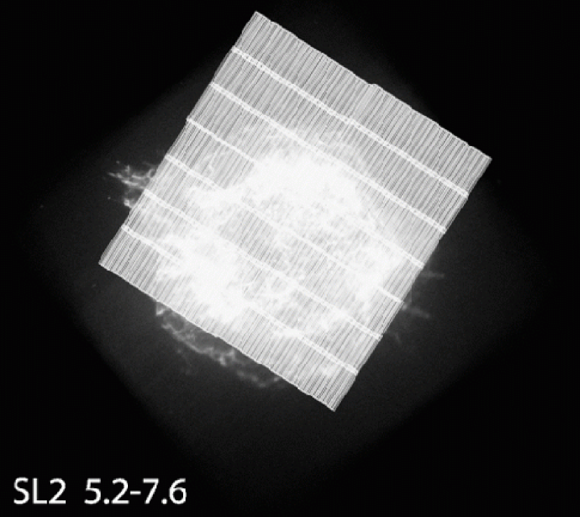
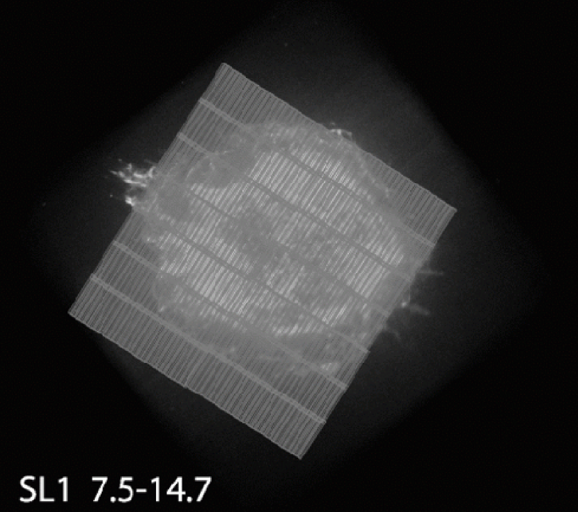
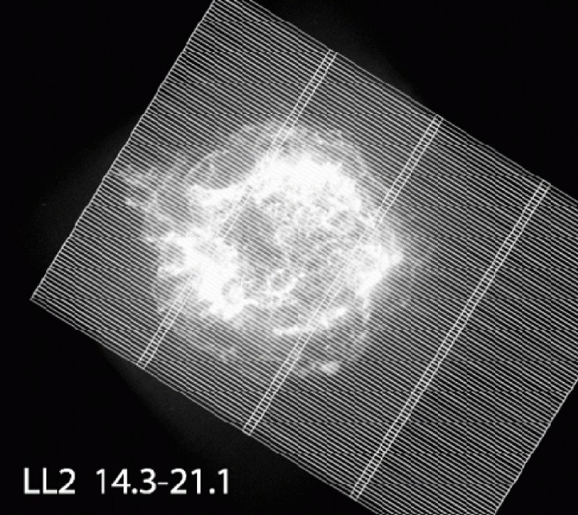
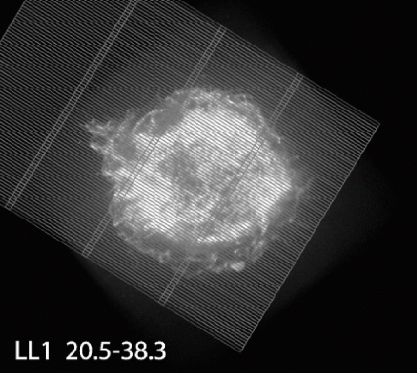
Figure 1: The slit positions for the Spitzer IRS mapping overlaid on the Chandra broadband X-ray image. The wavelength ranges in microns are indicated for each of the short-low (SL) and long-low (LL) orders.

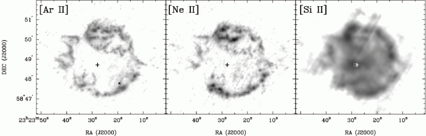
Figure 2: Left: 6.99 µm [Ar II] image and center: 12.81 µm [Ne II] image showing the Bright Ring. Right: 34.8 µm [Si II] image showing the Diffuse Interior Emission. For reference, the location of the central compact object is denoted by the crosses. The [Ar II] spectrum in Figure 4 was extracted from the small box region on the southwest Bright Ring. The [Si II] spectrum in Figure 4 was extracted from the central box near the CCO.

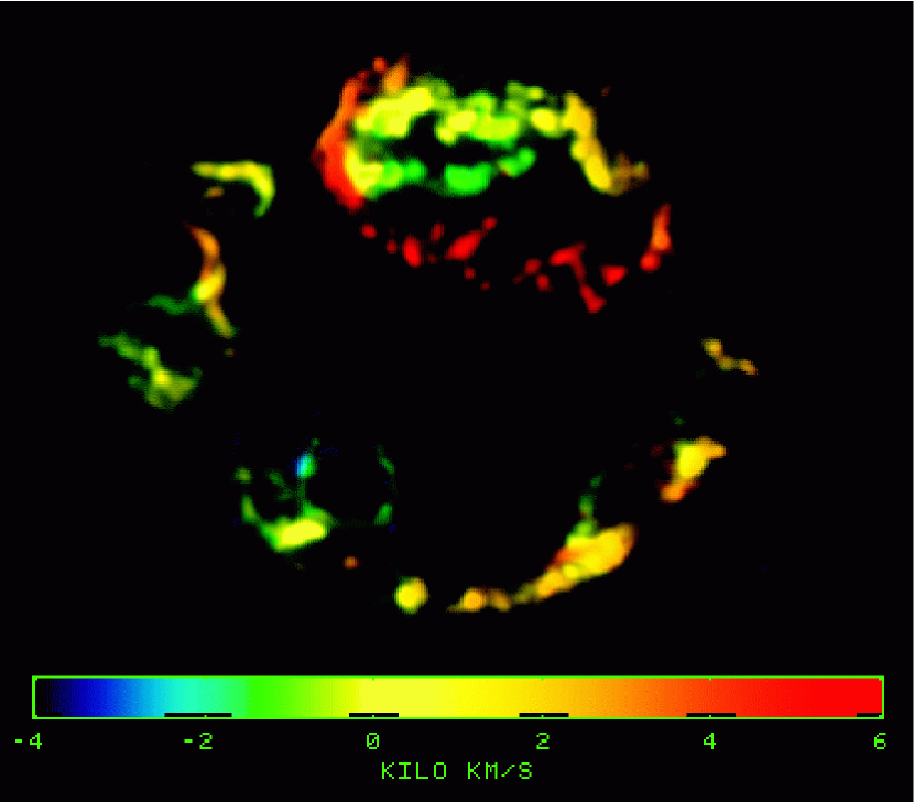
Figure 3: 1st moment map for [Ar II] showing the major Doppler structures that define the Bright Ring. Note that in locations with more than one Doppler component, the color represents a brightness-weighted average velocity.

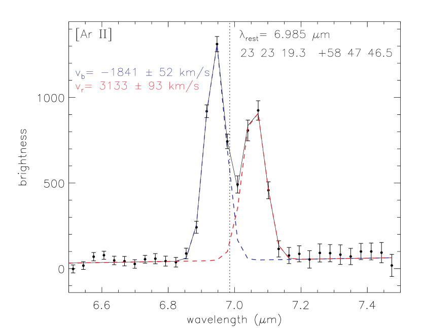
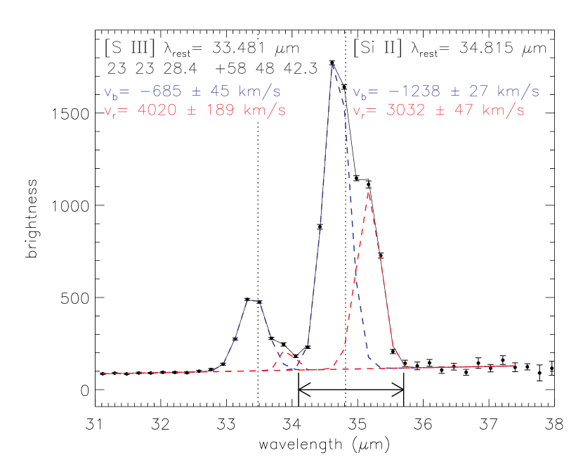
Figure 4: Top: Gaussians plus continuum fit (solid line) to the [Ar II] emission in a region on the Bright Ring (see Figure 2) with 2 line-of-sight Doppler components (dashed red and blue lines). Bottom: Joint Gaussians plus continuum fit to the [S III] and [Si II] emission in a region near the center of the remnant (see Figure 2), each with 2 line-of-sight Doppler components. The velocities of the blue ($v_{b}$) and red ($v_{r}$) components are indicated with 1-$\sigma$ statistical errors. The rest wavelengths of the [Ar II], [S III], and [Si II] lines are indicated by the vertical dotted lines. The wavelength range plotted in Figure 5 is indicated at the bottom of the plot.

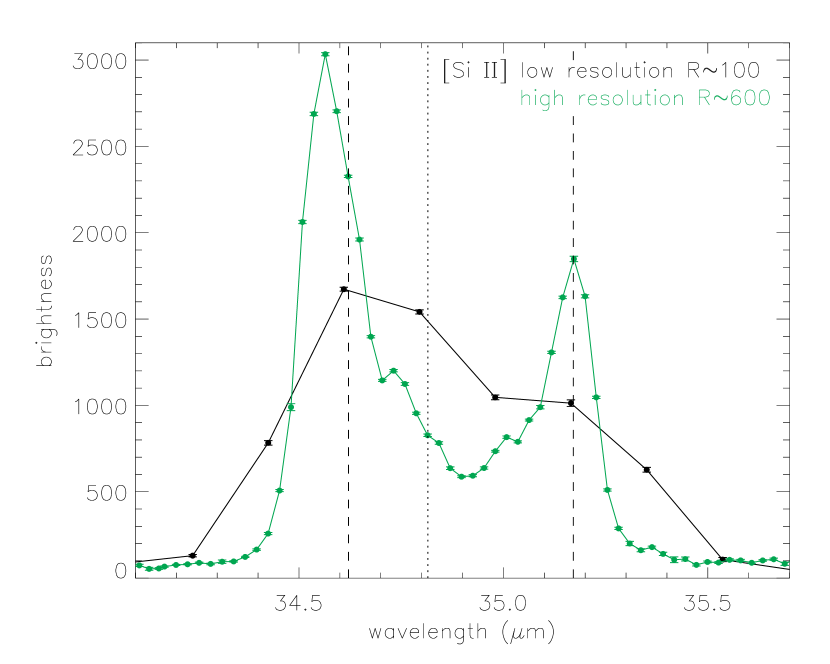
Figure 5: High-resolution [Si II] spectrum (green) from same region as the right panel of Figure 4 showing two primary Doppler components with smaller velocity structures extending to the center of the remnant. The low-resolution spectrum is plotted in black for comparison and the low-resolution line centroids are indicated by the vertical dashed lines. The vertical dotted line denotes the rest wavelength of [Si II].

Figure 6: HETG-derived Si Doppler velocity compared to ACIS-derived Si Doppler velocity for the sample of 17 ejecta knots measured by Lazendic et al. (2006). The best-fit straight line to the data is shown and indicates both a velocity scaling and offset between the two data sets. The rest wavelength used to compute the ACIS velocities was 6.648Å.

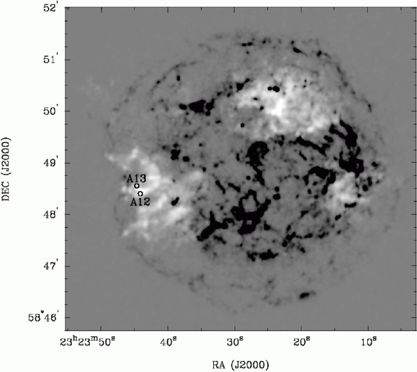
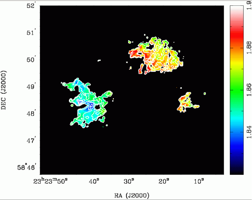
Figure 7: Left: Spectral tomography image showing the Fe-K emission as positive brightness. The spectra from regions A12 and A13 of Hwang & Laming (2003) are shown in Figure 8. Right: Effective Doppler map showing the fitted Gaussian line centers measured in Ångstroms. The approximate velocity range is $\pm 4000$ km s^-1, however ionization effects are not accounted for. The contours represent brightness levels on the spectral tomography image.

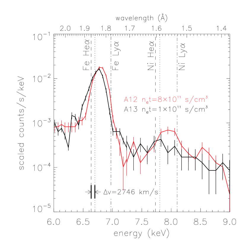
Figure 8: X-ray spectra for regions A12 and A13 of Hwang & Laming (2003) (marked in Figure 7) showing the Fe-K and Ni-K emission lines. The higher ionization age of region A12 results in an apparent blueshift in the spectrum. The rest wavelengths of the dominant Fe-K and Ni-K He$\alpha$ forbidden (dashed line) and resonance (dotted line) lines and Ly$\alpha$ lines (dot-dashed line) are indicated. At the bottom of the plot, we show that a shift of 0.017Å corresponds to an apparent Doppler shift of 2746 km s^-1.

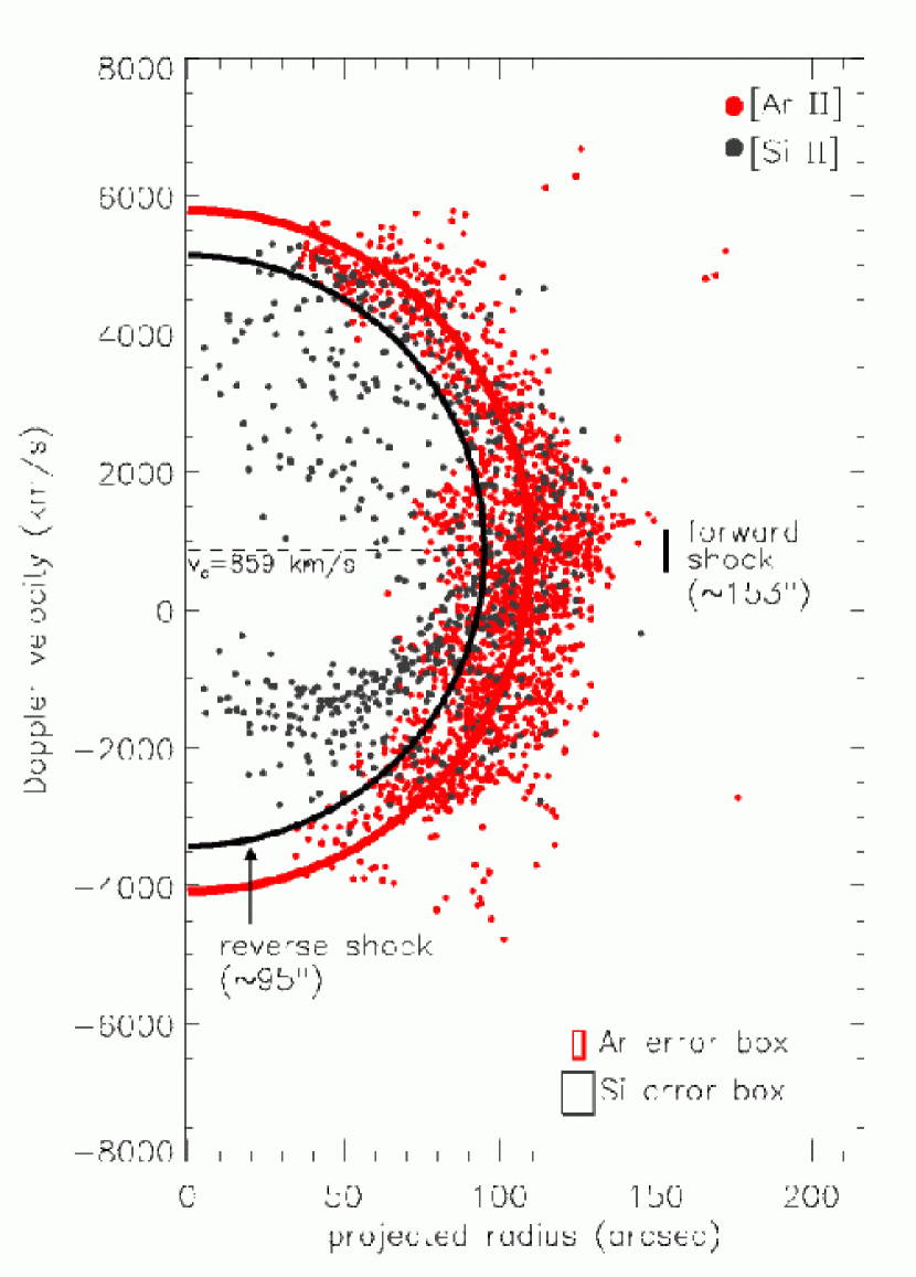
Figure 9: Doppler velocity vs. projected radius for [Ar II] in red and [Si II] in grey. The mean velocity errors and spatial resolution are indicated by error boxes at the bottom of the figure. The red semicircle represents the best-fit spherical expansion model. The black semicircle represents the reverse shock and the projected radius of the forward shock is also indicated. Note that the center of the spherical expansion model is not at zero velocity.

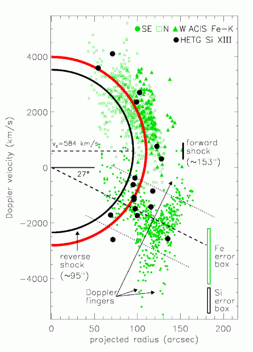
Figure 10: Doppler velocity vs. projected radius for Fe-K in green and HETG Si XIII in black. Different symbols are used to represent the north (open square), west (filled triangle), and southeast (filled circle) Fe-K distributions. The mean velocity errors and spatial resolution are indicated by error boxes at the bottom of the figure. The red semicircle represents the best-fit spherical expansion model from Figure 9, but scaled appropriately for the decelerated X-ray ejecta. The black semicircle represents the reverse shock in this decelerated reference frame. The forward shock projected radius is indicated at 153$\arcsec$. A few Doppler fingers that are due to ionization effects are identified. These correspond to fingers 1-3 in Figure 14.

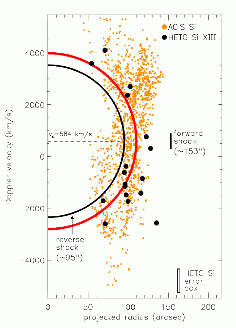
Figure 11: Doppler velocity vs. projected radius for ACIS Si in orange and HETG Si XIII in black. The mean velocity error and spatial resolution for the HETG data is indicated by the error box at the bottom of the figure. The red semicircle represents the best-fit spherical expansion model from Figure 9, but scaled appropriately for the decelerated X-ray ejecta. The black semicircle represents the reverse shock in this decelerated reference frame. The forward shock projected radius is indicated at 153$\arcsec$.

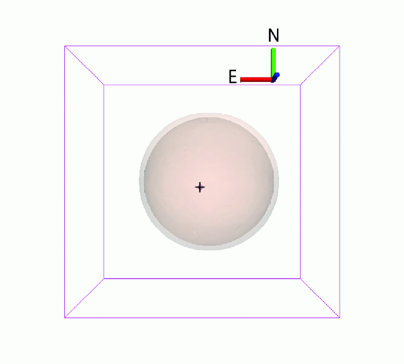
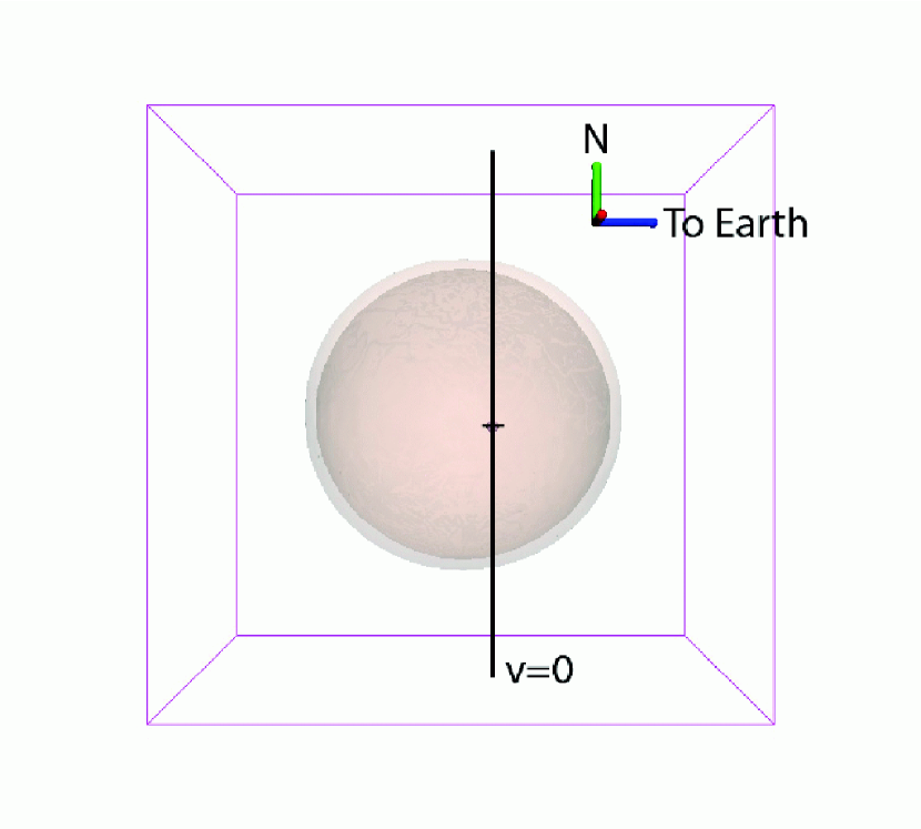
Figure 12: Three-dimensional projections showing the fiducial reverse shock (sphere) and CCO (cross) as seen from Earth (left) and from a 90$\arcdeg$ rotation to the east (right). The location where ejecta Doppler velocities=0 is identified in the right panel. Here and in subsequent 3D projections, the coordinate system is identified at upper right in each panel with red=east, green=north and blue=to Earth. The color-coding for this and subsequent 3D projections is described in Table The Three-Dimensional Structure of Cassiopeia A.

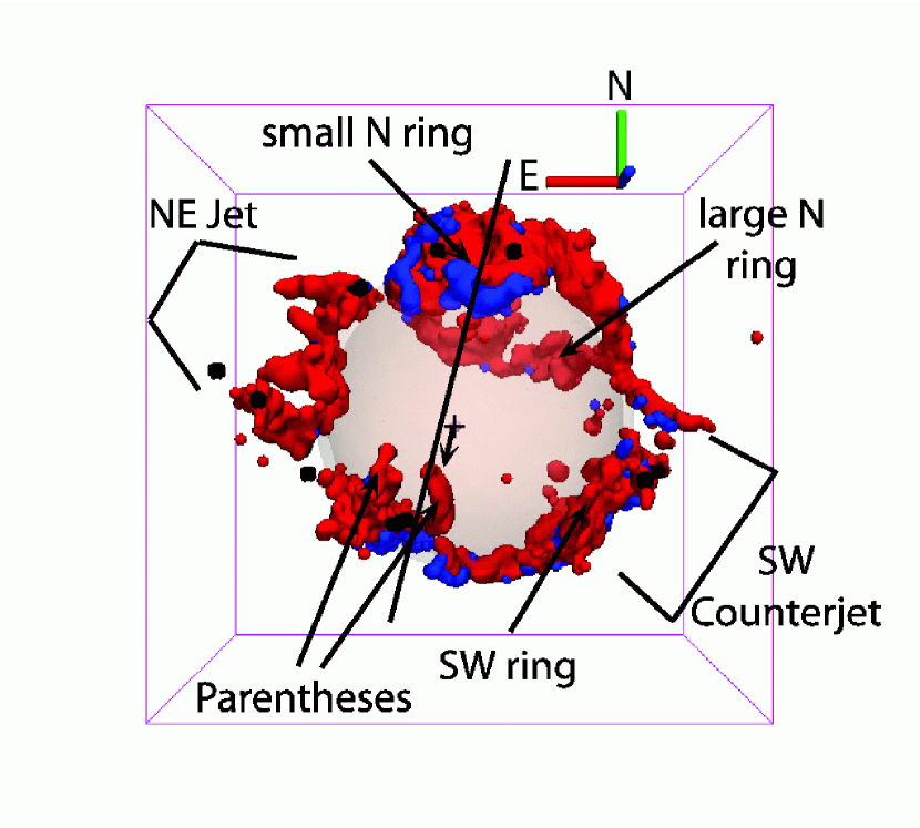
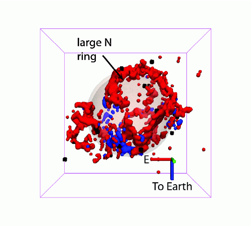
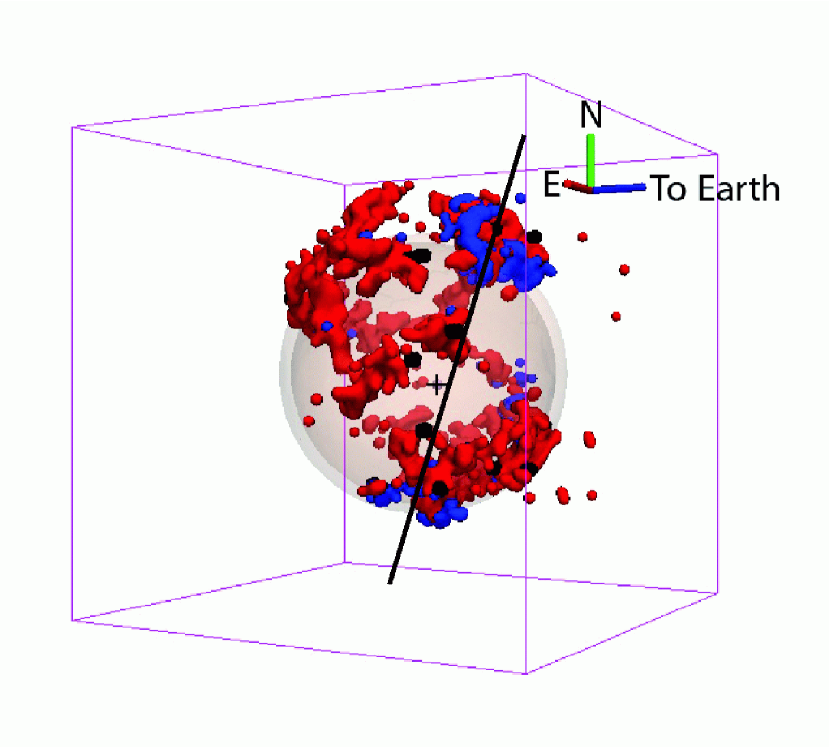
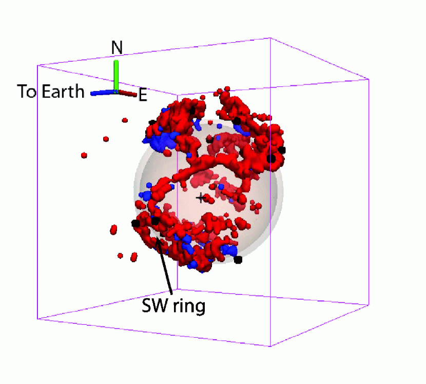
Figure 13: Three-dimensional projections of the infrared [Ar II] emission (red), X-ray Si XIII emission (black), the fiducial reverse shock (sphere), and the CCO (cross). Locations where the [Ne II]/[Ar II] ratio are high are indicated in blue. The lines in the top left and bottom left panels identify an apparent symmetry axis for the Ne-rich regions. The inferred CCO proper motion direction is indicated in the top left panel. Major structures discussed in §4.3 are indicated. The individual views are: top left - from Earth, top right - from the north, bottom left - 60$\arcdeg$ rotation to the east, bottom right - 120$\arcdeg$ rotation to the west. These same four projections will be used for all subsequent 3D figures.

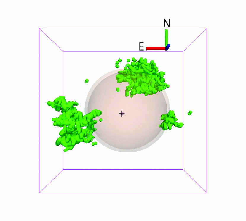
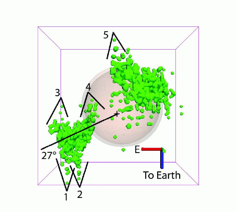
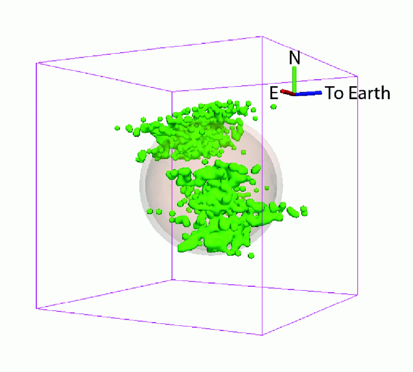
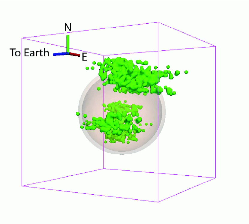
Figure 14: Three-dimensional projections of the X-ray Fe-K emission (green) with the reverse shock (sphere) and CCO (cross). Regions 1-5 in the upper right panel identify red- and blue-shifted Doppler fingers that result from ionization effects. The Doppler fingers in the southeast Fe-K complex (1-4) were collimated to lie along the 27$\arcdeg$ line.

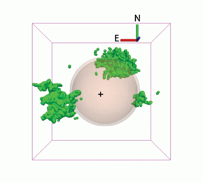
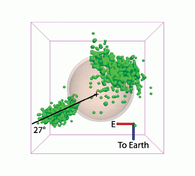
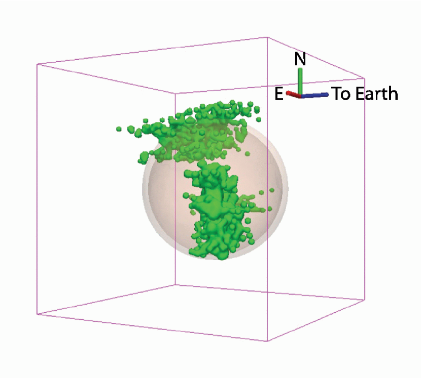
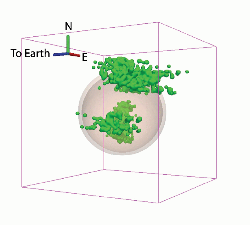
Figure 15: Three-dimensional projections of the ionization corrected X-ray Fe-K emission with the reverse shock (sphere) and CCO (cross).

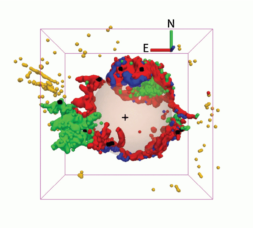
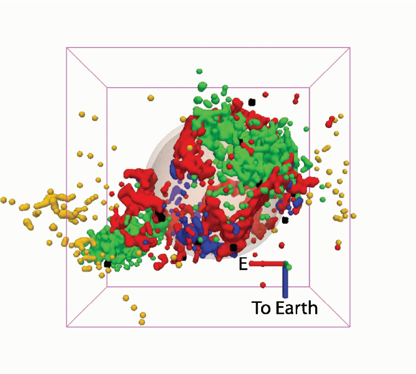
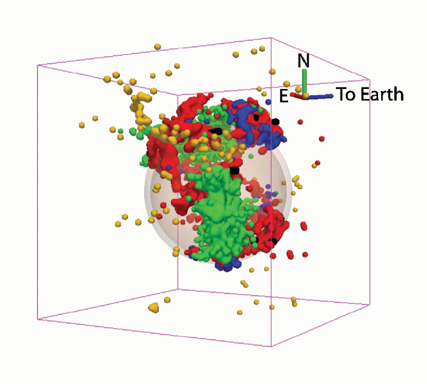
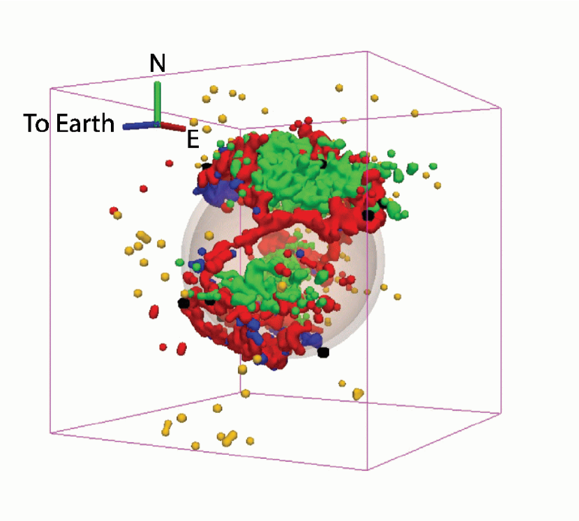
Figure 16: Three-dimensional projections of the infrared [Ar II] (red), high infrared [Ne II]/[Ar II] ratio (blue), X-ray Si XIII (black), X-ray Fe-K (green), outer optical ejecta (yellow), fiducial reverse shock (sphere), and CCO (cross). The fastest moving outer optical ejecta defining the northeast Jet and southwest Counterjet may have moved as much as 12$\arcsec$ in the intervening years, which is about twice the size of the plotting symbols.

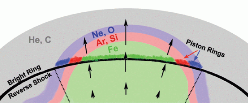
Figure 17: Cross-section of a simple ejecta piston model in which the layering of the progenitor star has been preserved. At the intersection between the wedge-shaped piston and reverse shock, shock-heated Fe is enclosed by a ring of shock-heated Ne/O and Ar/Si emission. Interior to the reverse shock, the Fe sits within a hole in the unshocked Si distribution. The center of the piston is moving faster than the edges of the piston accounting for the Fe layer having crossed the reverse shock in the center while the Ne/O and Ar/Si layers are just now reaching the reverse shock at the edges. All of the ejecta currently crossing the reverse shock have velocities of $\approx 5000$ km s^-1.

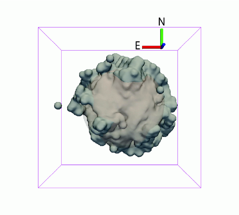
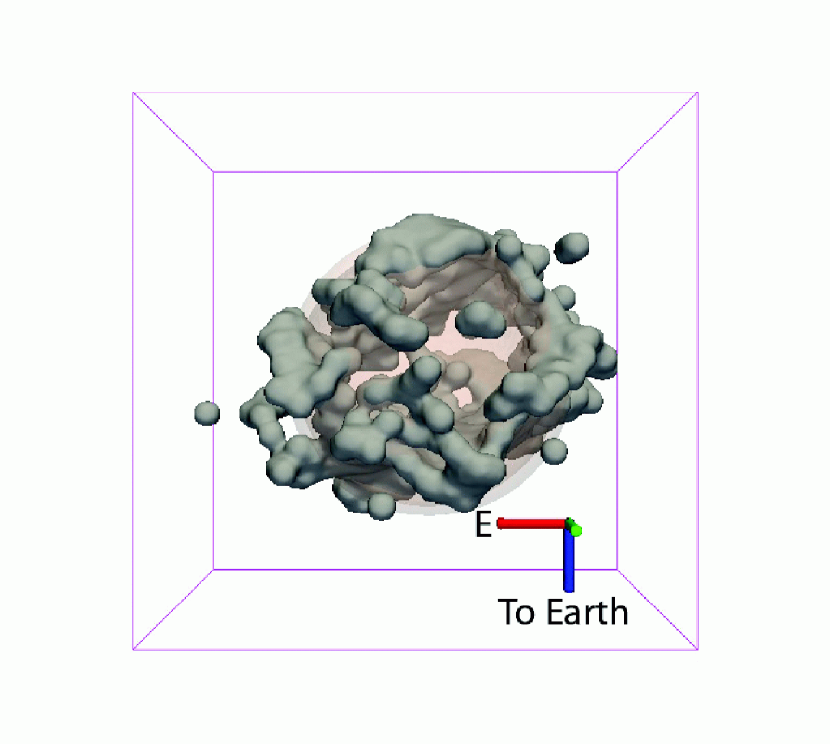
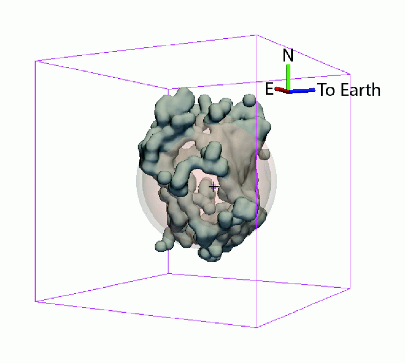
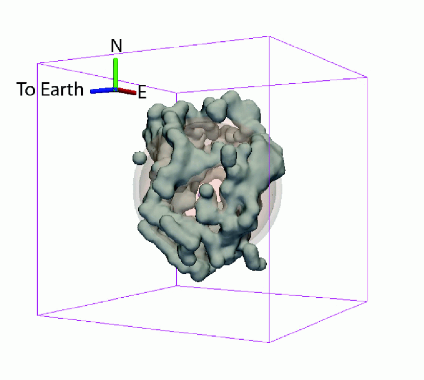
Figure 18: Three-dimensional projections of the infrared [Si II] emission (grey), fiducial reverse shock (sphere) and CCO (cross). There are two populations of [Si II] ejecta – a shocked population that resides on the Bright Ring and an unshocked population that is physically interior to the reverse shock.

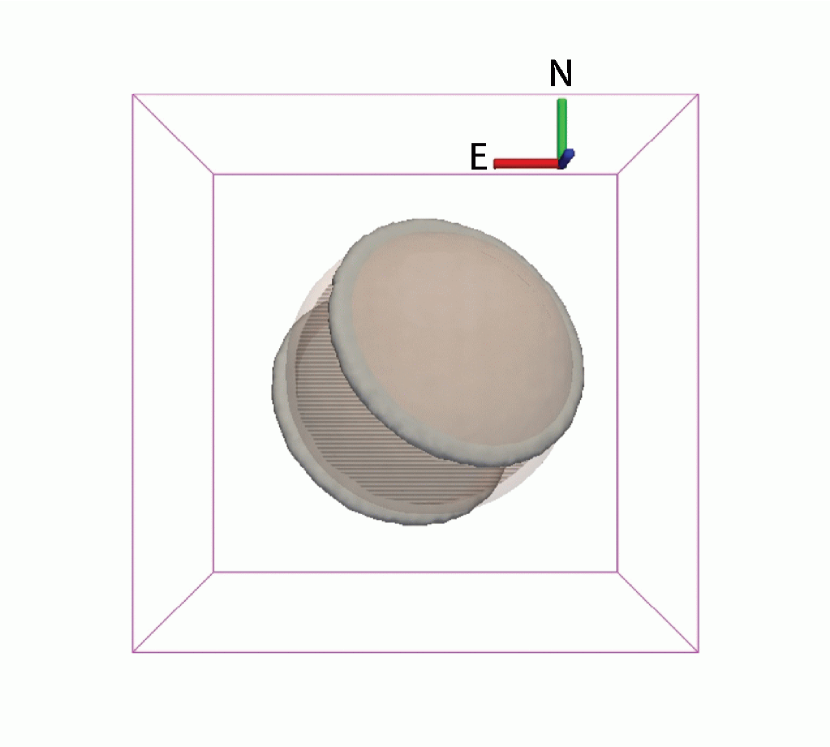
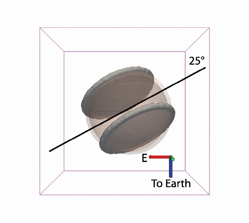
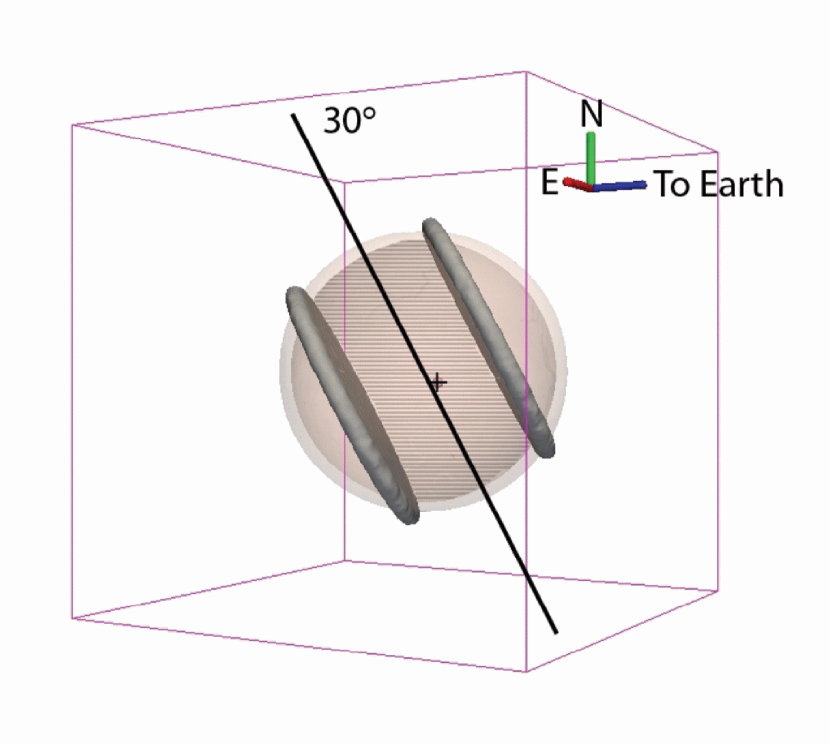
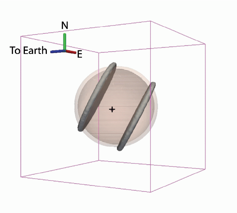
Figure 19: Three-dimensional projections showing the tilted thick disk model (grey and hashed) with the fiducial reverse shock (sphere) and the CCO (cross). The hash marks between the faces indicate that the region is not empty but contains weak emission from unshocked Si, S, and O and probably undetected unshocked Fe. Approximate orientations with respect to the north-south and east-west axes are indicated.

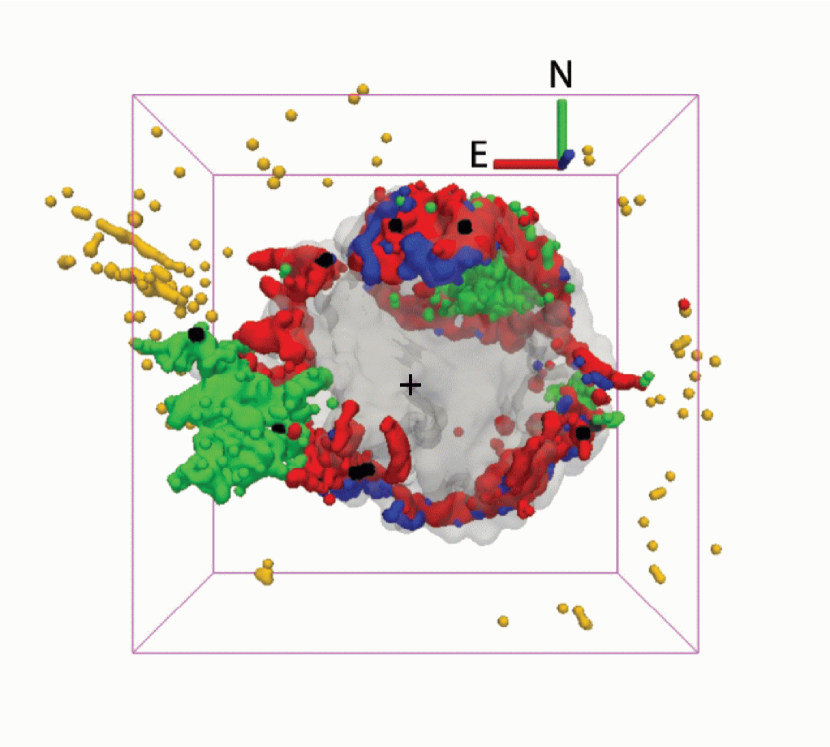
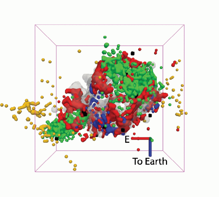
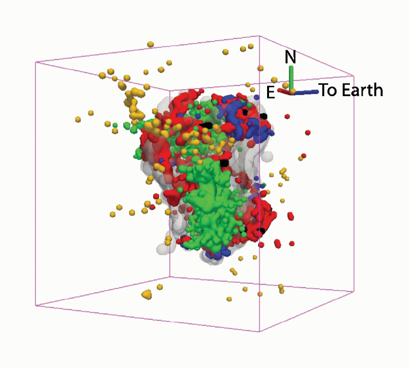
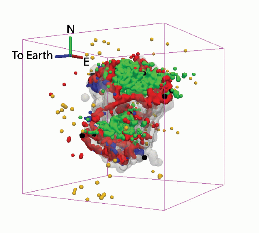
Figure 20: Three-dimensional projections of the infrared [Ar II], high [Ne II]/[Ar II] ratio, and [Si II] emission, the X-ray Fe-K and Si XIII emission, and the outer optical knots. The color coding is described in Table The Three-Dimensional Structure of Cassiopeia A. This figure is also available as an mpeg animation and a 3D PDF in the electronic edition of the Astrophysical Journal. The mpeg animation and 3D PDF are also available at http://homepages.spa.umn.edu/${}_{\textrm{\~{}}}$tdelaney/paper.

Figure 21: Grayscale: 34.48 µm [Si II] emission smoothed to 20$\arcsec$ resolution; Red contours: X-ray Fe-K emission; Blue contours: optical H$\alpha$ and [N II] emission from diffuse and clumpy CSM. The green lines denote the linear northeast jet structures and the green circle identifies the location of the outermost optical ejecta observed by Fesen et al. (2006). The edges of the LL1 slit mapping shown in Figure 1 are indicated.

References

- Akiyama et al. (2003) Akiyama, S., Wheeler, J. C., Meier, D., & Lichtenstadt, I. 2003, ApJ, 584, 954
- Arendt, Dwek, & Moseley (1999) Arendt, R. G., Dwek, E., & Moseley, S. H. 1999, ApJ, 521, 234
- Bisnovatyi-Kogan & Blinnikov (1982) Bisnovatyi-Kogan, G. S. & Blinnikov, S. I. 1982, Soviet Ast., 26, 530
- Blondin et al. (2003) Blondin, J. M., Mexxacappa, A. & DeMarino, C. 2003, ApJ, 584, 971
- Braun, Gull, & Perley (1987) Braun, R., Gull, S. F., & Perley, R. A. 1987, Nature, 327, 395
- Burrows et al. (2005) Burrows, A., Walder, R., Ott, C. & Livne, E. 2005, in ASP Conf. Ser. 332, ed. R. M. Humphreys & K.Z. Stanek (San Francisoco: ASP), 350
- Burrows et al. (2007) Burrows, A., Dessart, L., Ott, C. D. & Livne, E. 2007, Phys. Rep., 442, 23
- Burrows (2009) Burrows, A. 2009, KITP Conference: Stellar Death and Supernovae (August 17-21, 2009), http://online.kitp.ucsb.edu/online/sdeath_c09/burrows/
- Chevalier (1976) Chevalier, R. 1976, ApJ, 208, 826
- Chevalier & Kirshner (1979) Chevalier, R. & Kirshner, R. 1979, ApJ, 233, 154
- Chevalier & Soker (1989) Chevalier, R. & Soker, N. 1989, ApJ, 341, 867
- Davis et al. (2005) Davis, J. E., Houck, J. C., Allen, G. E., & Stage, M. D. 2005, in ASP Conf. Ser. 347, Astronomical Data Analysis Software and Systems XIV, ed. P. Shopbell, M. Britton, & R. Ebert (San Francisco: ASP), 444
- DeLaney & Rudnick (2003) DeLaney, T. & Rudnick, L. 2003, ApJ, 589, 818
- DeLaney et al. (2004) DeLaney, T., Rudnick, L., Fesen, R. A., Jones, T. W., Petre, R., & Morse, J. A. 2004, ApJ, 613, 343
- Dohm-Palmer & Jones (1996) Dohm-Palmer, R. & Jones, T. W. 1996, ApJ, 471, 279
- Ennis et al. (2006) Ennis, J. A., Rudnick, L., Reach, W. T., Smith, J. D., Rho, J., DeLaney, T., Gomez, H., & Kozasa, T. 2006, ApJ, 652, 376
- Fesen (2001) Fesen, R. A. 2001, ApJS, 133, 161
- Fesen et al. (2001) Fesen, R. A., Morse, J. A., Chevalier, R. A., Borkowski, K. J., Gerardy, C. L., Lawrence, S. S., & van den Bergh, S. 2001, AJ, 122, 2644
- Fesen & Gunderson (1996) Fesen, R. A. & Gunderson, K. S. 1996, ApJ, 470, 967
- Fesen et al. (2006) Fesen, R. A., Hammell, M. C., Morse, J., Chevalier, R. A., Borkowski, K. J., Dopita, M. A., Gerardy, C. L., Lawrence, S. S., Raymond, J. C., & van den Bergh, S. 2006, ApJ, 645, 283
- Fesen, Pavlov, & Sanwal (2006) Fesen, R. A., Pavlov, G. G., & Sanwal, D. 2006, ApJ, 636, 848
- Gerardy & Fesen (2001) Gerardy, C. L. & Fesen, R. A. 2001, AJ, 121, 2781
- Gnat & Sternberg (2006) Gnat, O. & Sternberg, A. 2007, ApJ, 168, 213
- Gotthelf et al. (2001) Gotthelf, E. V., Koralesky, B., Rudnick, L., Jones, T. W., Hwang, U., & Petre, R. 2001, ApJ, 552, L39
- Hamilton & Fesen (1998) Hamilton, A. J. S. & Fesen, R. A. 1998, ApJ, 327, 178
- Hamilton et al. (1997) Hamilton, A. J. S., Fesen, R. A., Wu, C.-C., Crenshaw, D. M., & Sarazin, C. L. 1997, ApJ, 481, 838
- Hammell & Fesen (2009) Hammell, M. C. & Fesen, R. A. 2008, ApJS, 179, 195
- Hammer, Janka, & Mueller (2010) Hammer, N. J., Janka, H.-Th., & Mueller, E. 2010, ApJ, 714, 1371
- Hines et al. (2004) Hines, D. C. et al. 2004, ApJS, 154, 290
- Holt et al. (1994) Holt, S. S., Gotthelf, E. V., Tsunemi, H., & Negoro, H. 1994, PASJ, 46, L151
- Houck & Denicola (2000) Houck, J. C. & Denicola, L. A. 2000, in ASP Conf. Ser. 216, Astronomical Data Analysis Software and Systems IX, ed. N. Manset, C. Veillet, & D. Crabtree (San Francisco: ASP), 591
- Hughes et al. (2000) Hughes, J. P., Rakowski, C. E., Burrows, D. N., & Slane, P. O. 2000, ApJ, 528, L109
- Hwang, Holt, & Petre (2000) Hwang, U., Holt, S., & Petre, R. 2000, ApJ, 537, L119
- Hwang et al (2001) Hwang, U., Szymkowiak, A. E., Petre, R., & Holt, S. S. 2001, ApJ, 560, L175
- Hwang & Laming (2003) Hwang, U. & Laming, J. M. 2003, ApJ, 597, 362
- Hwang & Laming (2009) Hwang, U. & Laming, J. M. 2009, ApJ, 703, 883
- Hwang et al. (2004) Hwang, U., et al. 2004, ApJ, 615, L117
- Isensee et al. (2010) Isensee, K., et al. 2010, ApJin press (arXiv:1006.0918)
- Janka et al. (2005) Janka, H.-Th., Scheck, L., Kifonidis, K., Müller, E. & Plewa, T. 2005, in ASP Conf. Ser. 332, eds. R. M. Humphreys & K. S. Stanek (San Francisco: ASP), 363
- Joggerst, Woosley & Heger (2009) Joggerst, C. C., Woosley, S. E., & Heger, A. 2009, ApJ, 693, 1780
- Kamper & van den Bergh (1976) Kamper, K. & van den Bergh, S. 1976, ApJS, 32, 351
- Kassim et al. (1995) Kassim, N. E., Perley, R. A., Dwarakanath, K. S., & Erickson, W. C. 1995, ApJ, 455, L59
- Kifonidis et al. (2003) Kifonidis, K., Plewa, T., Janka, H.-Th. & Müller, E. 2003, A&A408, 621
- Kifonidis et al. (2006) Kifonidis, K., Plewa, T., Scheck, L., Janka H.-Th. & Müller, E. 2006, A&A, 453, 661
- Krause et al. (2008) Krause, O., Birkmann, S. M., Usuda, T., Hattori, T., Goto, M., Rieke, G. H., & Misselt, K. A. 2008, Science, 320, 1195
- Laming & Hwang (2003) Laming, J. M. & Hwang, U. 2003, ApJ, 597, 347
- Laming et al. (2006) Laming, J. M., Hwang, U., Radics, B., Lekli, G., & Takács, E. 2006, ApJ, 644, 260
- Lawrence et al. (1995) Lawrence, S. S., MacAlpine, G. M., Uomoto, A., Woodgate, B. E., Brown, L. W., Oliverson, R. J., Lowenthal, J. D., & Liu, C. 1995, AJ, 109, 2635
- Lazendic et al. (2006) Lazendic, J. S., Dewey, D., Schultz, N. S., & Canizares, C. R. 2006, ApJ, 651, 250
- Markert et al. (1983) Markert, T. H., Canizares, C. R., Clark, G. W., & Winkler, P. F. 1983, ApJ, 268, 134
- Mazzali et al. (2005) Mazzali, P. et al. 2005, Science, 308, 1284
- Milisavljevic & Fesen (2010) Milisavljevic, D. & Fesen, R. 2010, BAAS, 42, 469
- Minkowski (1959) Minkowski, R. 1959, IAU Symposium, 9, 315
- Moiseenko, Bisnovatyi-Kogan & Gennady (2007) Moiseenko, S., Bisnovatyi-Kogan & Gennady, S. 2007, Ap&SS, 311, 191
- Morse et al. (2004) Morse, J. A., Fesen, R. A., Chevalier, R. A., Borkowski, K. J., Gerardy, C. L., Lawrence, S. S., & van den Bergh, S. 2004, ApJ, 614, 727
- Patnaude & Fesen (2007) Patnaude, D. & Fesen, R. 2007, AJ, 133, 147
- Predehl & Schmitt (1995) Predehl, P. & Schmitt, J. H. M. M. 1995, A&A, 293, 889
- Rampp & Janka (2000) Rampp, M. & Janka, H.-T. 2000, ApJ, 539, L33
- Reed et al. (1995) Reed, J. E., Hester, J. J., Fabian, A. C., & Winkler, P. F. 1995, ApJ, 440, 706
- Rest et al. (2008) Rest, A. et al. 2008, ApJ, 681, L81
- Rest et al. (2010) Rest, A. et al. 2010, ApJ, submitted (arXiv:1003.5660)
- Rho et al. (2008) Rho, J., Kozasa, T., Reach, W. T., Smith, J. D., Rudnick, L., DeLaney, T., Ennis, J. A., Gomez, H., & Tappe, A. 2008, ApJ, 673, 271
- Rho et al. (2003) Rho, J., Reynolds, S. P., Reach, W. T., Jarrett, T. H., Allen, G. E., & Wilson, J. C. 2003, ApJ, 592, 299
- Scheck et al. (2004) Scheck, L., Plewa, T., Janka, H.-Th., Kifonidis, K., & Müller, E. 2004, Phys. Rev. Lett., 92, 011103
- Schure et al. (2008) Schure, K. M., Vink, J., Garcia-Segura, G., & Achterberg, A. 2008, ApJ, 686, 399
- Shklovsky (1979) Shklovsky, I. S. 1979, Nature, 279, 703
- Smith et al. (2007a) Smith, J. D., Armus, L., Dale, D. A., Roussel, H., Sheth, K., Buckalew, B. A., Jarret, T. H., Helou, G., & Kennicutt, R. C. 2007, PASP, 119, 1133
- Smith et al. (2007b) Smith, N., Li, W., Foley, R., Wheeler, J. C., Pooley, D., Chornock, R., Filippenko, A., Silverman, J., Quimby, R., Bloom, J. & Hansen, C. 2007, ApJ, 666, 1116
- Smith et al. (2009) Smith, J. D. et al. 2009, ApJ, 693, 713
- Smith & Townsend (2007) Smith, N. & Townsend, R. 2007, ApJ, 666, 967
- Stage et al. (2004) Stage, M. D., Allen G. E., Houck, J. C., & Davis, J. E. 2004, BAAS, 36, 948
- Stage et al. (2006) Stage, M. D., Allen G. E., Houck, J. C., & Davis, J. E. 2006, NatPh, 2, 614
- Tanaka et al. (2008) Tanaka, M., Kawabata, K., Maeda, K., Hattori, T. & Nomoto, K. 2008, ApJ, 689, 1191
- Thorstensen, Fesen, & van den Bergh (2001) Thorstensen, J. R., Fesen, R. A., & van den Bergh, S. 2001, AJ, 122, 297
- Truelove & McKee (1999) Truelove, J. K. & McKee, C. F. 1999, ApJS, 120, 299
- van den Bergh & Dodd (1970) van den Bergh, S. & Dodd, W. W. 1970, ApJ, 162, 485
- van den Bergh & Kamper (1983) van den Bergh, S. & Kamper, K. 1983, ApJ, 268, 129
- van den bergh & Kamper (1985) van den Bergh, S. & Kamper, K. 1985, ApJ, 293, 537
- Wang et al. (2001) Wang, L., Howell, D. Höflich, P. & Wheeler, J. C. 2001, ApJ, 550, 1030
- Wang et al. (2002) Wang, L. et al. 2002, ApJ, 579, 671
- Wang, Baade & Patat (2007) Wang, L., Baade, D. & Patat, F. 2007, Science, 315, 212
- Wheeler, Maund, & Couch (2008) Wheeler, J. C., Maund, J. R., & Couch, S. M. 2008, ApJ, 677, 1091
- Willingale et al. (2002) Willingale, R., Bleeker, J. A. M., van der Heyden, K. J., Kaastra, J. S., & Vink, J. 2002, A&A, 381, 1039
- Willingale et al. (2003) Willingale, R., Bleeker, J. A. M., van der Heyden, K. J., & Kaastra, J. S. 2003, A&A, 398, 1021
- Woosley (1988) Woosley, S. E. 1988, ApJ, 330, 218
- Yang, Lu, & Chen (2008) Yang, X.-J., Lu, F.-J., & Chen, Li 2008, Chinese J. Astron. Astrophys., 8, 439
- Zhang, Woosley & Heger (2004) Zhang, W., Woosley, S. & Heger, A. 2004, ApJ, 608, 365