We propose a strategy to demonstrate the transition from the quantum Zeno effect (QZE) to the anti-Zeno effect (AZE) using a superconducting qubit coupled to a transmission line cavity, by varying the central frequency of the cavity mode. Our results are obtained without the rotating wave approximation (RWA), and the initial state (a dressed state) is easy to prepare. Moreover, we find that in the presence of both qubit’s intrinsic bath and the cavity bath, the emergence of the QZE and the AZE behaviors relies not only on the match between the qubit energy level spacing and the central frequency of the cavity mode, but also on the coupling strength between the qubit and the cavity mode.
Keywords: Quantum Zeno effect, anti-Zeno effect, qubit, cavity

The transition from quantum Zeno to anti-Zeno effects for a qubit in a cavity by varying the cavity frequency

I Introduction

The QZE predicts that the decay rate of a system can be slowed down by measuring it frequently enough pra-41-2295 ; pra-42-5720 ; pra-44-1466 ; pascazio . However some systems are predicted to have an enhancement of the decay due to the frequent measurements, namely the AZE or inverse Zeno effect nature-405-546 ; p ; q . The QZE and AZE have been observed in an unstable system prl-87-040402 .

Recently, the QZE-AZE crossover in quantum Brownian motion model was investigated prl-97-130402 , where a system of damped harmonic oscillator interacts with a bosonic reservoir in thermal equilibrium. It was found prl-97-130402 that controlling the system-environment coupling by an artificially-controllable engineered environment (e.g., nature-407-57 ; nature-403-269 ) would allow one to monitor the transition from the QZE to the AZE dynamics. The QZE and AZE of a nanomechanical resonator measured by a quantum point contact detector (non-equilibrium fermionic reservoir) also was studied prb-81-115307 . Therefore, modulating the system and reservoir parameters can induce the QZE-AZE crossover.

In cavity QED, the coupling between the qubit and the cavity, in which the electromagnetic field modes are concentrated around the cavity resonant frequency, depends on the cavity frequency. For an excited qubit located in a cavity, the cavity mode is the dominant one available for the qubit to emit photons. If the qubit energy level spacing is resonant with the cavity mode, the rate of decay into the particular cavity mode is enhanced. Otherwise, it is inhibited. Therefore, one may manipulate the qubit decay rate by varying the central frequency of the cavity mode in or off resonance with the qubit level energy spacing. The variation of the qubit decay pra-81-062131 ; pra-54-R3750 in the cavity is an increasingly important topic for experimental and theoretical studies prl-85-2272 ; prl-101-180402 ; pra-81-062131 .

In this paper, we propose to modulate the qubit’s decay rate in cavity QED by the QZE, which means invoke the frequent measurements in the qubit and achieve the transition between QZE and AZE. We study a model of a qubit in a cavity, and investigate the occurrence of either the QZE or AZE by varying the cavity central frequency. We insert frequent projection measurements in the qubit decay process and find that the normalized decay rate depends on whether the central frequency of the cavity mode is in resonance with the qubit energy level spacing or not. In the resonant case, the normalized decay rate is lower than 1, so the QZE of the qubit occurs. However, when the cavity mode is detuned from the energy level spacing of the qubit, the normalized decay rate is larger than 1 and the qubit exhibits AZE. The variation from the QZE to the AZE, by varying the central frequency of the cavity mode, should help distinguishing these two kinds of effects. Moreover, we consider the case when both the qubit’s intrinsic bath and the cavity bath are simultaneously present. And find the dependence of the behaviors (the QZE and the AZE) on the coupling strength of the qubit-cavity and the cavity central frequency.

The QZE-AZE crossover may be achieved in a superconducting qubit coupled to a transmission line cavity jqyou ; prl-103-147003 ; pra-81-042304 ; pra-69-062320 . This is because there are two physical mechanisms to tune the resonant frequency of the transmissionline resonator. One method is to change the boundary condition of the electromagnetic field in the transmission line prb-74-224506 ; apl-92-203905 ; apl-93-042510 , as shown in the Fig. 1(a). Another method is to construct a transmission line resonator by using a series of magnetic-flux biased SQUIDs, as shown in the Fig. 1(b). Because the effective inductor of a magnetic-flux-biased SQUID can be tuned by changing the applied magnetic flux nature-4-929 ; apl-91-083509 , the inductance per unit length of the SQUID array is controllable.

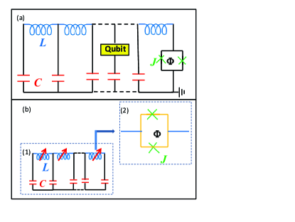
Figure 1: (Color online) (a) Superconducting circuit model of a frequency-tunable transmission line resonator, which is archived by changing the boundary condition, coupled with a qubit. (b) Superconducting circuit model (1) of the effective tunable inductors, which are consisted of a series array of SQUIDs (2).

II Hamiltonian of a qubit in a cavity beyond the rotating wave approximation

Including the qubit dissipation environment, the Hamiltonian of a qubit in a lossy cavity can be written as

$$H = \frac{1}{2}\Delta\sigma_{z}+\sum_{k}\omega_{k,1}b_{k}^{\dagger}b_{k}+\sum_{k}f_{k}(b_{k}^{\dagger}+b_{k})\sigma_{x}$$ (1)

$$+\sum_{k}\omega_{k,2}a_{k}^{\dagger}a_{k}+\sum_{k}g_{k}(a_{k}^{\dagger}+a_{k})\sigma_{x}.$$

The Pauli operators, $\sigma_{z}$ and $\sigma_{x},$ describe the qubit level energy spacing and tunneling. The operators $b_{k}$ and $b_{k}^{\dagger}$ are the annihilation and creation operators characterizing the qubit’s intrinsic bath with frequencies $\omega_{k,1}$. The lossy cavity is modeled as a collection of harmonic oscillators with frequencies $\omega_{k,2},$ with the creation operators $a_{k}^{\dagger}$ and the annihilation operators $a_{k}$. Figure 2(a) schematically shows the model considered here.

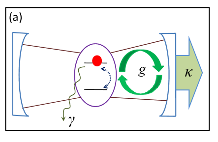
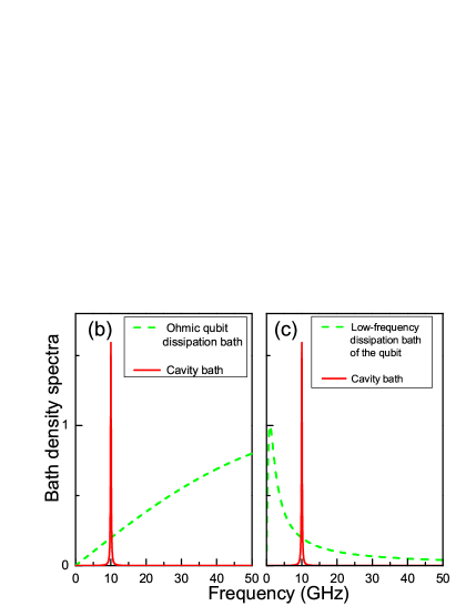
Figure 2: (Color online) (a) Sketch of a qubit with the spontaneous dissipation rate $\gamma$ coupled to a cavity with the loss rate $\kappa$ via a coupling strength $g.$ (b) and (c) schematically show the bath density spectrum of the qubit environment: (b) the Ohmic qubit’s intrinsic bath (green dashed) and the Lorentzian cavity bath (red solid), (c) the low-frequency qubit’s intrinsic bath (green dashed) and the Lorentzian cavity bath (red solid).

Notice that no RWA is invoked in the Hamiltonian $H$ and thus it can not be diagonalized exactly.

Now let us solve the Schrödinger equation of the Hamiltonian (1). We take the anti-rotating terms into account, which guarantees that our discussions extend to the off-resonant regime and also the case when there is a strong qubit-cavity interaction. Due to the anti-rotating terms, we apply a unitary transformation to the Hamiltonian $H$,

$$H^{\prime}=\exp(S)H\exp\left(-S\right),$$ (2)

with

$$S=\sum_{k}\left[\frac{f_{k}}{\omega_{k,1}}\xi_{k,1}(b_{k}^{\dagger}-b_{k})+\frac{g_{k}}{\omega_{k,2}}\xi_{k,2}(a_{k}^{\dagger}-a_{k})\right]\sigma_{x}.$$ (3)

Here, the $k$-dependent variables

$$\xi_{k,1}=\omega_{k,1}/(\omega_{k,1}+\eta_{1}\;\Delta),$$ (4)

and

$$\xi_{k,2}=\omega_{k,2}/(\omega_{k,2}+\eta_{2}\;\Delta),$$ (5)

are introduced in the transformation. The transformed Hamiltonian $H^{\prime}$ can be written as

$$H^{\prime} \approx \frac{1}{2}\eta\;\Delta\sigma_{z}+\sum_{k}\omega_{k,1}b_{k}^{\dagger}b_{k}+\sum_{k}\omega_{k,2}a_{k}^{\dagger}a_{k}$$ (6)

$$+\sum_{k}V_{k,1}(b_{k}^{\dagger}\sigma_{-}+b_{k}\sigma_{+})$$

$$+\sum_{k}V_{k,2}(a_{k}^{\dagger}\sigma_{-}+a_{k}\sigma_{+}),$$

with $\sigma_{\pm}=\left(\sigma_{x}\pm i\sigma_{y}\right)/2$ and

$$\eta=\eta_{1}\>\eta_{2}.$$ (7)

Then, the qubit energy-level-spacing $\Delta$ is renormalized to $\eta\;\Delta$ because of its coupling to the qubit’s intrinsic bath and the cavity bath. These factors $\eta_{1}$ and $\eta_{2},$ are respectively denoted by

$$\eta_{1} = \exp\left(-\sum_{k}2f_{k}^{2}\xi_{k,1}^{2}{}/\omega_{k,1}^{2}\right),$$ (8)

$$\eta_{2} = \exp\left(-\sum_{k}2g_{k}^{2}\xi_{k,2}^{2}{}/\omega_{k,2}^{2}\right).$$ (9)

The coupling constants $f_{k}$ and $g_{k},$ of the qubit-environment interaction are also renormalized. The renormalized factors are respectively denoted by

$$V_{k,1} = 2\eta_{1}\;\Delta\;f_{k}/\left(\omega_{k,1}+\eta_{1}\;\Delta\right),$$ (10)

$$V_{k,2} = 2\eta_{2}\;\Delta\;g_{k}/\left(\omega_{k,2}+\eta_{2}\;\Delta\right),$$ (11)

owing to the anti-rotating coupling terms. In Eq. (6), we drop the higher-order terms, which include the induced effect of the two baths by the coupling to the same qubit $\mathcal{O}$$\left(f_{k}\cdot g_{k}\right)$, whose contributions to the physical quantities are of the order $\mathcal{O}$$\left(g_{k}^{4}\right)$ $\left[\text{or }\mathcal{O}\left(f_{k}^{4}\right),\text{ or }\mathcal{O}\left(f_{k}^{2}g_{k}^{2}\right)\right]$ and higher.

III Equation of motion of a qubit in a cavity beyond the rotating wave approximation

Below, we will solve the equation of motion of the wave function, beyond the RWA, in the transformed Hamiltonian $H^{\prime}$ in Eq. (6). Since the total excitation number operator

$$N=\sum_{k}\left(a_{k}^{\dagger}a_{k}+b_{k}^{\dagger}b_{k}\right)+\left(1+\sigma_{z}\right)/2,$$ (12)

of the dissipative qubit-cavity system is a conserved observable, i.e., $\left[N,H^{\prime}\right]=0,$ it is reasonable to restrict our discussion to the single-particle excitation subspace. A general state in this subspace can be written as

$$\left|\Phi(t)\right\rangle=\chi(t)\left|\uparrow\right\rangle\left|\{0_{k}\;0_{k}\}\right\rangle+\sum_{k,i}\beta_{k,i}(t)\left|\downarrow\right\rangle\left|\{0_{k,\overline{i}}\;1_{k,i}\}\right\rangle,$$ (13)

where $\left|\uparrow\right\rangle$ and $\left|\downarrow\right\rangle$ are the eigenstates of $\sigma_{z}$ ($\sigma_{z}\left|\uparrow\right\rangle=\left|\uparrow\right\rangle$ and $\sigma_{z}\left|\downarrow\right\rangle=-\left|\downarrow\right\rangle$), the state $\left|\{0_{k,\overline{i}}\;1_{k,i}\}\right\rangle$ ($i$ can be $1,2$) means that either the cavity bath or the qubit’s intrinsic bath has one quantum excitation. Substituting $\left|\Phi(t)\right\rangle$ into the Schrödinger equation, we have

$$i\frac{d\chi(t)}{dt}=\frac{\eta\;\Delta}{2}\chi(t)+\sum_{k,i}V_{k,i}\;\beta_{k,i}(t),$$ (14)

$$i\frac{d\beta_{k,i}(t)}{dt}=\left(\omega_{k,i}-\frac{\eta\;\Delta}{2}\right)\beta_{k,i}(t)+\sum_{k,i}V_{k,i}\;\chi(t).$$ (15)

Applying the transformation

$$\chi(t)\! \!=\! \!\widetilde{\chi}(t)\exp\left(-i\frac{\eta\;\Delta}{2}t\right),$$ (16)

$$\beta_{k,i}(t)\! \!=\! \!\widetilde{\beta}_{k,i}(t)\exp\left[-i\left(\omega_{k,i}-\frac{\eta\;\Delta}{2}\right)t\right],$$ (17)

Eqs. (14) and (15) is simplified as

$$\frac{d\widetilde{\chi}(t)}{dt}\!=\!-i\sum_{k,i}V_{k,i}\;\widetilde{\beta}_{k,i}(t)\exp\left[-i(\omega_{k,i}-\eta\;\Delta)t\right],$$ (18)

$$\frac{d\widetilde{\beta}_{k,i}(t)}{dt}=-iV_{k,i}\;\widetilde{\chi}(t)\exp\left[i(\omega_{k,i}-\eta\;\Delta)t\right].$$ (19)

Integrating Eq. (19) and substituting it into Eq. (18), we obtain

$$\frac{d\widetilde{\chi}(t)}{dt}=-\int\limits_{0}^{t}\sum_{k,i}V_{k,i}^{2}\exp\left[-i(\omega_{k,i}-\eta\;\Delta)(t-t^{\prime})\right]\;\widetilde{\chi}(t^{\prime})\;dt^{\prime}.$$ (20)

This integro-differential equation can be solved exactly by a Laplace transformation,

$$\overline{\widetilde{\chi}(p)}=\frac{\widetilde{\chi}(0)}{p+\sum_{k,i}V_{k,i}^{2}/\left[p-i(\eta\;\Delta-\omega_{k,i})\right]},$$ (21)

with

$$\overline{\widetilde{\chi}(p)}=\int\widetilde{\chi}(t)\exp(-pt)dt.$$ (22)

Inversing of the Laplace transformation, we obtain the amplitude in the excited-state

$$\widetilde{\chi}(t)=\frac{1}{2\pi i}\int_{\sigma-i\infty}^{\sigma+i\infty}\frac{\widetilde{\chi}(0)\exp(pt)}{p+\sum_{k,i}V_{k,i}^{2}/\left[p-i(\eta\;\Delta-\omega_{k,i})\right]}dp$$ (23)

Then replace $p$ to $i\omega+0^{+},$

$$\widetilde{\chi}(t)=\frac{1}{2\pi i}\int_{-\infty}^{\infty}\frac{\widetilde{\chi}(0)\exp(i\omega t)}{\omega-\sum_{k,i}V_{k,i}^{2}/\left[(\omega+\eta\;\Delta)-\omega_{k,i}-i0^{+}\right]}d\omega$$ (24)

Denote $R(\omega)$ and $\Gamma(\omega)$ as the real and imaginary parts of the summation term $\sum_{k,i}V_{k,i}^{2}/(\omega-\omega_{k,i}-i0^{+}),$ then

$$R(\omega) = \wp\sum_{k,i}V_{k,i}^{2}/(\omega-\omega_{k,i}-i0^{+})$$ (25)

$$\Gamma(\omega) = \pi\sum_{k,i}V_{k,i}^{2}\delta(\omega-\omega_{k,i}-i0^{+})$$ (26)

where $\wp$ is the Cauchy principal value. Applying the pole approximation,

$$\widetilde{\chi}(t)=\widetilde{\chi}(0)\sum_{j}\exp(i\omega_{j}t)Q_{j}(\omega_{j})$$ (27)

where $\omega_{j}$ corresponds to the singularity of the quantity $\overline{\widetilde{\chi}(p)}$ and $Q_{j}(\omega_{j})$ is the normalized factor.

Before doing further calculations, let us now focus on the initial state of the system $\widetilde{\chi}(0)$, since different initial states may result in distinct predictions about the QZE and the AZE PRL-101-200404 ; pra-ai . Indeed, these two effects can strongly depend on the initial conditions. Through the unitary transformation in Eq. (2), the Hamiltonian (1), which contains the anti-rotating terms, is reduced to $H^{\prime}$ in Eq. (6), which has the similar form of the Hamiltonian under the RWA, with the parameters renormalized. Under energy conservation, the ground state of $H^{\prime}$ is $\left|g^{\prime}\right\rangle=\left|\downarrow\right\rangle\left|\{0_{k}\;0_{k}\}\right\rangle$ and the corresponding ground-state energy is $-\eta\;\Delta/2$. Therefore, through inversing the unitary transformation, we obtain the ground state of the original Hamiltonian $H$ as $\left|g\right\rangle=\exp[-S]\left|\downarrow\right\rangle\left|\{0_{k}\;0_{k}\}\right\rangle,$ which is a dressed state of the qubit and its environment due to the anti-rotating terms prl-103-147003 ; pra-80-053810 . In this paper, we choose the excited state $\exp[-S]\left|\uparrow\right\rangle\left|\{0_{k}\;0_{k}\}\right\rangle$ as the initial state, which can be achieved by acting the operator $\sigma_{x}$ on the ground state,

$$\left|\psi(0)\right\rangle=\sigma_{x}\left|g\right\rangle=\exp[-S]\left|\uparrow\right\rangle\left|\{0_{k}\;0_{k}\}\right\rangle.$$ (28)

Thus, the initial state after the transformation is $\left|\psi^{\prime}(0)\right\rangle=\left|\uparrow\right\rangle\left|\{0_{k}\;0_{k}\}\right\rangle$, correspondingly the excited-state probability amplitude $\chi(0)=1.$

To obtain the final result, we need the knowledge of the interacting spectra of the qubit’s intrinsic bath and also the cavity bath. From the quasi-mode approach, the qubit-cavity coupling density spectrum is a Lorentzian density spectrum pra-71-032302 ; a

$$J_{\mathrm{cav}}(\omega)=\sum g_{k,2}^{2}\delta(\omega-\omega_{k})=\frac{g^{2}\;\lambda}{\pi[(\omega-\omega_{\mathrm{cav}})^{2}+\lambda^{2}]},$$ (29)

where $g$ is the coupling constant between the cavity and the qubit, $\omega_{\mathrm{cav}}$ the central frequency of the cavity mode, and $\lambda$ is the frequency width of the cavity bath density spectrum and is related to the cavity bath correlation time. The physical quantity $\omega_{\mathrm{cav}}/\lambda$ denotes the quality factor $Q$ of the cavity.

Experiments in some superconducting qubits indicate that the noise chiefly comes from the low-frequency region. The density spectrum of the low-frequency bath can be approximately written as

$$J_{\mathrm{qb}}^{\mathrm{low}}(\omega)=\sum_{k}g_{k,2}^{2}\delta(\omega-\omega_{k,1})=\frac{2\;\alpha_{\mathrm{low}}\;\omega}{\left(\omega/\Delta\right)^{2}+\left(\omega_{\mathrm{low}}/\Delta\right)^{2}}.$$ (30)

where $\omega_{\mathrm{low}}$ is an energy lower than the qubit energy spacing $\Delta$, and $\alpha_{\mathrm{low}}$ a dimensionless coupling strength between the qubit and the intrinsic bath. In semiconductor quantum dot qubits, the qubit spontaneous dissipation bath, mainly the phonon bath, is usually described by an Ohmic density spectrum. Thus, the density spectrum $J_{\mathrm{qb}}(\omega)$ of the Ohmic bath with Drude cutoff can be given as

$$J_{\mathrm{qb}}^{\mathrm{Ohm}}(\omega)=\sum_{k}g_{k,1}^{2}\delta(\omega-\omega_{k,1})=\frac{2\;\alpha_{\mathrm{Ohm}}\;\omega}{1+\left(\omega/\omega_{\mathrm{Ohm}}\right)^{2}},$$ (31)

where $\omega_{\mathrm{Ohm}}$ is the high-frequency cutoff, which is typically assumed to be larger than the qubit energy level spacing, and $\alpha_{\mathrm{Ohm}}$ is the dimensionless coupling strength.

So we consider three kinds of interacting density spectra: Lorentzian cavity bath, low-frequency qubit’s intrinsic bath and Ohmic qubit’s intrinsic bath, and present a sketch of the density spectra of the qubit environment in Fig. 2(b, c): showing the same cavity bath and different qubit’s intrinsic baths (a low-frequency bath in (b) and an Ohmic bath in (c)).

Figure 3: (Color online) Time dependence of the probability for the qubit at its excited state. In the resonant case, the parameters are $\omega_{\mathrm{cav}}=\Delta=100~{}g$ and $\tau=0.1~{}g^{-1}$. In the detuning case, the cavity mode frequency is varied to $\omega_{\mathrm{cav}}=80~{}g$. Note that the successive measurements slow down the decay rate of excited state in the resonant case, which is the QZE. While in the detuning case, the measurements speed up the qubit decay rate, which is the AZE.

Before illustrate our results, let us recall the standard master equation of a qubit coupled to a single-mode cavity under the RWA and Markov approximation pra-40-5516

$$\dot{\rho} = -i\left[H_{\mathrm{RWA}},\rho\right]+\gamma\left(2\sigma_{-}\rho\sigma_{+}-\sigma_{+}\sigma_{-}\rho-\rho\sigma_{+}\sigma_{-}\right)$$ (32)

$$+\kappa\left(2a\rho a^{\dagger}-a^{\dagger}a\rho-\rho a^{\dagger}a\right),$$

where $H_{\mathrm{RWA}}=g(\sigma_{-}a^{\dagger}+\sigma_{+}a),$ $g$ is the qubit-cavity coupling strength, $a^{\dagger}$ and $a$ are the creation and annihilation operators for the single-mode cavity. The two parameters $\kappa$ and $\gamma$ correspond to the decay rates induced by the two baths: the qubit’s intrinsic bath and the cavity bath, respectively. Then the survival probability of the qubit in the excited state is approximately pra-40-5516

$$P_{\mathrm{e}}(t)=\left|\chi(t)\right|^{2}\;=\cos\left(gt\right)\exp\left[-\left(\kappa+\gamma\right)t/2\right],$$ (33)

where the subscript “$\mathrm{e}$” refers to the initial and final excited states. The exponential factor $\left(\kappa+\gamma\right)/2$ can be considered as an effective decay rate. In the RWA case, the qubit energy is splitting to $\Delta\pm g/2.$

While in our results beyond the RWA, the qubit energy splitting depends on the qubit environment. Assume $\lambda=0.1~{}g,$ $\omega_{\mathrm{cav}}=100~{}g.$ If the qubit in the low-frequency bath with $\omega_{\mathrm{low}}=10~{}g$ and $\alpha_{\mathrm{low}}=10^{-4}$, the qubit energy is splitting to $\Delta-0.4786~{}g$ and $\Delta+0.5011~{}g.$ While, if the qubit in the Ohmic bath with $\omega_{\mathrm{Ohm}}=10^{3}~{}g$ and $\alpha_{\mathrm{Ohm}}=10^{-4},$ the qubit energy level is splitting to $\Delta-0.5018~{}g$ and $\Delta+0.4782~{}g.$

Figure 3 shows the probability $P_{\mathrm{e}}(t)$ for the qubit to be in the excited state in the region $0<t<\pi$. When the qubit and the cavity mode is resonant, the qubit decay with the measurements, whose interval between successive measurements is $\tau=0.1~{}g^{-1},$ is slowed down compared to the case without measurement (the interval $\tau$ extends to infinite), which means QZE. While tune the cavity mode to $\omega_{\mathrm{cav}}=80~{}g$ and fix the energy level spacing of the qubit $\Delta=100~{}g$, the decay with the measurements ($\tau=0.1~{}g^{-1}$) is speeded up contrast to the case without the measurements, which means AZE.

IV The effective decay rate of a qubit in a cavity with successive measurements

In the following, we will solve the Eq. (20) iteratively and obtain the effective decay rate with successive measurement pra-54-R3750 ; A10 . When the interval between measurements is sufficiently short, the evolution of the qubit after measurements can be approximately expressed by an exponential form. So the discussion in nature-405-546 can be extended to damped oscillations. Namely, if the exponential factor is larger or smaller than the effective decay rate $\left(\kappa+\gamma\right)/2,$ then the measurements reduce or enhance the decay rate. After the first iteration, Eq. (20) is solved as

$$\widetilde{\chi}(t)\simeq 1-\int\limits_{0}^{t}(t-t^{{}^{\prime}})\sum_{k,i}V_{k,i}^{2}\exp[-i(\omega_{k,i}-\eta\;\Delta)t^{{}^{\prime}}]\;dt^{{}^{\prime}}.$$ (34)

For a small $t$, we can approximately write $\widetilde{\chi}(t)$ in an exponential form:

$$\widetilde{\chi}(t) = \exp\left[-\int\limits_{0}^{t}(t-t^{{}^{\prime}})\sum_{k,i}V_{k,i}^{2}\exp\left[-i(\omega_{k,i}-\eta\;\Delta)t^{{}^{\prime}}\right]dt^{{}^{\prime}}\right]$$ (35)

$$= \exp\left\{-t\left[-\frac{1}{t}\sum_{k,i}V_{k,i}^{2}\frac{\exp\left[-i\left(\omega_{k,i}-\eta\;\Delta\right)t\right]-1+i\left(\omega_{k,i}-\eta\;\Delta\right)t}{\left(\omega_{k,i}-\eta\;\Delta\right)^{2}}\right]\right\}$$

$$= \exp\left\{-t\left[\sum_{k,i}V_{k,i}^{2}\left(\frac{2\sin\left(\frac{\omega_{k,i}-\eta\;\Delta}{2}t\right)^{2}}{t\left(\omega_{k,i}-\eta\;\Delta\right)^{2}}-i\frac{\left(\omega_{k,i}-\eta\;\Delta\right)t-\sin\left[\left(\omega_{k,i}-\eta\;\Delta\right)t\right]}{t\left(\omega_{k,i}-\eta\;\Delta\right)^{2}}\right)\right]\right\}.$$

Note that only when $\tau\ll g^{-1},$ the qubit evolution can be approximately described as an exponential decay pra-40-5516 ; pra-54-R3750 ; pra-81-062131 , which has been reflected in Fig. 2. Assume now that the instantaneously-ideal projection measurement is performed periodically, separated by time intervals $\tau$. For a single measurement, the probability amplitude of the qubit maintaining in the initial state is $\widetilde{\chi}(t=\tau).$ After a sufficiently large number of measurements, the survival probability of the initial state becomes

$$P_{\mathrm{e}}(t=n\tau)\;=\;\left|\widetilde{\chi}(t=n\tau)\right|^{2}\;=\;\exp[-\gamma(\tau)t].$$ (36)

And the exponential decay constant $\gamma(\tau)$ is obtained

$$\gamma(\tau) = 2\pi\int_{0}^{\infty}d\omega\sum_{k,i}V_{k,i}^{2}\;\frac{2\sin^{2}(\frac{\eta\;\Delta-\omega}{2}\tau)}{\pi(\eta\;\Delta-\omega)^{2}\tau}$$ (37)

$$= 2\pi\int_{0}^{\infty}d\omega J(\omega)f(\omega)F(\omega-\eta\;\Delta,\tau),$$

where

$$f(\omega)=\left(1-\frac{\omega-\eta\;\Delta}{\omega+\eta\;\Delta}\right)^{2},$$ (38)

$$J(\omega) = \sum_{k}\left[f_{k}^{2}\delta(\omega-\omega_{k,1})+g_{k}^{2}\delta(\omega-\omega_{k,2})\right]$$ (39)

$$= J_{\mathrm{cav}}(\omega)+J_{\mathrm{qb}}(\omega),$$ (40)

and

$$F(\omega-\eta\;\Delta,\tau)=\frac{2\sin^{2}\left[\left(\eta\;\Delta-\omega\right)\tau/2\right]}{\pi(\eta\;\Delta-\omega)^{2}\tau}.$$ (41)

In Eq. (40), $J(\omega)$ is the entire interacting density spectrum with $J_{\mathrm{cav}}(\omega)$ from the cavity bath and $J_{\mathrm{qb}}(\omega)$ the qubit’s intrinsic bath. The function $F(\omega-\eta\;\Delta,\tau)$ comes from the projection measurements and can be called a modulating function of the measurements.

The decay rate $\gamma(\tau)$, in Eq. (37),  depends on the renormalization factor $\eta$ and $f(\omega)$ in Eq. (38), which are mainly from the anti-rotating terms. If we use the RWA, $\eta=1$ and $f(\omega)=1,$ which is consistent with the case of weak interaction. Therefore, our results can apply to not only the weak coupling case, but also to the case of strong coupling between the qubit and the environment. Furthermore, since the function $F(\omega-\Delta,\tau)$ becomes $\delta(\omega-\eta\;\Delta)$ in the long-time limit, we obtain the effective decay rate under the Weisskopf-Wigner approximation

$$\gamma_{0}=\gamma(\tau\rightarrow\infty)=2\pi J(\eta\;\Delta).$$ (42)

The normalized decay rate, which characterizes the QZE and the AZE, is determined by

$$\frac{\gamma(\tau)}{\gamma_{0}}=\frac{\int_{0}^{\infty}d\omega J(\omega)f(\omega)F(\omega-\eta\;\Delta,\tau)}{J(\eta\;\Delta)}.$$ (43)

For a finite time $\tau,$ and when $\gamma(\tau)/\gamma_{0}<1$ holds, we have the QZE, i.e., measurements hinder the decay. However, when $\gamma(\tau)/\gamma_{0}>1,$ this implies the AZE, i.e., measurements enhance the decay.

To see the contribution of each bath to the decay rate, Eq. (43) can be reexpressed as

$$\frac{\gamma(\tau)}{\gamma_{0}}$$ (44)

$$= \frac{J_{\mathrm{cav}}(\eta\;\Delta)}{J(\eta\;\Delta)}\frac{\int_{0}^{\infty}d\omega J_{\mathrm{cav}}(\omega)f(\omega)F(\omega-\eta\;\Delta,\tau)}{J_{\mathrm{cav}}(\eta\;\Delta)}$$

$$+\frac{J_{\mathrm{qu}}(\eta\;\Delta)}{J(\eta\;\Delta)}\frac{\int_{0}^{\infty}d\omega J_{\mathrm{qu}}(\omega)f(\omega)F(\omega-\eta\;\Delta,\tau)}{J_{\mathrm{qu}}(\eta\;\Delta)}.$$

From this Eq. (44), we see that the normalized decay rate due to the two baths is combined by the normalized decay rate from each bath by the weights $J_{\mathrm{qb}}(\eta\;\Delta)/J(\eta\;\Delta)$ and $J_{\mathrm{cav}}(\eta\;\Delta)/J(\eta\;\Delta),$ respectively.

V Results and Discussion

In this section, we will show the normalized decay rate of the qubit-cavity system in three cases: $\left(i\right)$ only the cavity bath, $\left(ii\right)$ both the cavity bath and the low-frequency qubit spontaneous dissipation bath coexist, as well as both the cavity bath and the Ohmic qubit’s intrinsic bath coexistence. According to the experiment nature-431-162 , we consider the qubit weakly coupled to the qubit intrinsic bath with coupling constants $\alpha_{\mathrm{Ohm}}=10^{-4}$ and $\alpha_{\mathrm{low}}=10^{-4}.$ The quality factor $Q$ of the cavity is assumed in the range of $2\times 10^{2}\sim 10^{4}$.

V.1 Only cavity bath

Let us first consider the case of a qubit only in a cavity bath. For example, when the qubit-cavity interaction $g\gg\alpha_{\mathrm{low}}\Delta,$ or $g\gg\alpha_{\mathrm{Ohm}}\Delta$, which has been realized in a superconducting qubit coupled to a transmission line cavity nature-458-178 ; add8 . For such strong coupling between the qubit and cavity, the normalized decay rate mainly depends on the cavity bath. Then in this case, the decay rate can be approximately written as

$$\gamma(\tau)=2\pi\int_{0}^{\infty}d\omega\;J_{\mathrm{cav}}(\omega)\;f(\omega)\;F(\omega-\eta\;\Delta,\tau).$$ (45)

From the normalized decay rate in Eq. (43), we see that the qubit-cavity coupling strength $g$ is in both, the numerator and denominator, so it cancels out. Therefore, the normalized decay rate $\gamma(\tau)$ is independent of the qubit-cavity coupling strength $g.$ However we still note that only in the case when $\tau\ll g^{-1},$ the qubit evolution can be approximately described by an exponential decay. This means that if there is a strong qubit-cavity coupling $g=0.1\Delta,$ the measurement interval becomes $\tau\ll g^{-1}\sim 10\Delta^{-1}.$ When the qubit-cavity is not so strong, $g=10^{-2}\Delta,$ the measurement interval could be $\tau\ll g^{-1}\sim 10^{2}\Delta^{-1}.$

Figure 4 displays the normalized decay rate as a function of the measurement interval $\tau$ and the cavity central frequency $\omega_{\mathrm{cav}}.$ Figures 4(a) and (b) correspond to two quality factors of the cavity: $Q=10^{4}$ and $Q=2\times 10^{3}$, respectively. We can see that in the limit when $\tau\rightarrow 0,$ only the QZE occurs.  For a finite interval, the normalized decay rate of the qubit exhibits a transition from the QZE to the AZE, by modulating the central frequency of the cavity mode $\omega_{\mathrm{cav}}$ in and off resonance with the qubit energy level spacing $\Delta$. The variation should be useful to distinguish the QZE and the AZE.

Let us now estimate the condition for the transition between the QZE and the AZE. From Fig. 4(a), the crossover from QZE to AZE, by varying the cavity frequency, appears only for the measurement interval $\tau>0.6\Delta^{-1}$. Using the condition $\tau\ll g^{-1}$, we obtain the qubit-cavity coupling strength $g\ll 1.7\Delta.$ Similarly, for the cavity quality factor $Q=2\times 10^{3},$ we obtain the qubit-cavity coupling strength $g\ll 0.38\Delta.$

In Fig. 5, we plot the normalized decay rate with the cavity frequency in resonance with the qubit, $\omega_{\mathrm{cav}}=\Delta$, versus the time interval $\tau$ between successive measurements, and the cavity spectral width $\lambda$. It is obvious that only the QZE exists in the resonant case. The normalized decay rate $\gamma(\tau)/\gamma_{0}$ becomes smaller as the cavity spectral width $\lambda$ decreases. This indicates that the transition from the QZE to the AZE becomes sharper as the cavity spectral width $\lambda$ reduces.

Figure 4: (Color online) Contour plots of the normalized decay rate $\gamma(\tau)/\gamma_{0}$ of the qubit only in the cavity bath, versus the time interval $\tau$ between successive measurements, and the central frequency $\omega_{\mathrm{cav}}$ of the cavity mode. (a) The width of the cavity frequency is $\lambda=10^{-4}\Delta$, and accordingly the cavity quality factor $Q=10^{4}.$ (b) The width of the cavity frequency $\lambda=5\times 10^{-3}\Delta$, corresponding to the cavity quality factor $Q=2\times 10^{3}$. The region $1\leq\gamma(\tau)/\gamma_{0}\leq 1.05$ is shown as light magenta. The QZE region corresponds to $\gamma(\tau)/\gamma_{0}<1$. The AZE region covers the rest, when $\gamma(\tau)/\gamma_{0}>1$. Evidently, a transition from the QZE to the AZE is observed by varying the central frequency of the cavity mode at finite $\tau$ ($\tau>0.6\Delta^{-1}$ when $Q=10^{4}$, and $\tau>2.6\Delta^{-1}$ when $Q=2\times 10^{3}$).

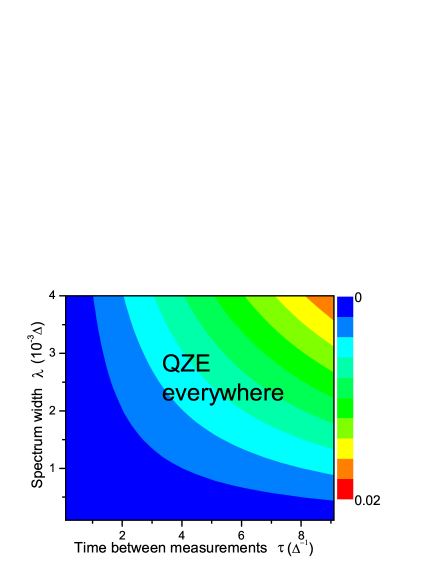
Figure 5: (Color online) Contour plots of the normalized effective decay rate $\gamma(\tau)/\gamma_{0}$ of the qubit in the resonant case $\Delta=\omega_{\mathrm{cav}}$.

To better understand the transition from the QZE to the AZE, we discuss the results in two regimes of near-resonance (including on-resonance) and off-resonance (the central frequency of the cavity mode higher and lower than the qubit spacing $\Delta$):

1. In the case of on-resonance $\Delta=\omega_{\mathrm{cav}},$ and near-resonance $\left|\Delta-\omega_{\mathrm{cav}}\right|<\lambda$, without measurements, the effective decay rate of the qubit is given by $J(\Delta).$ Moreover, the qubit is resonant with the cavity mode, $\Delta=\omega_{\mathrm{cav}}$. Note that $\omega_{\mathrm{cav}}$ is the peak of the density spectrum of the cavity-bath, where the probability of energy transfer from the qubit to the cavity bath is maximum. In this case, the qubit strongly decays in its evolution. Every measurement to project the qubit on the initial state protects the qubit from decay, i.e., protects the qubit from exchanging energy with the cavity. From Eq. (41), the modulating function $F(\omega-\eta\Delta,\tau)$ of the measurements is a periodically oscillating function versus energy $\omega$ for a fixed time interval $\tau$. Moreover, its integral over all energies is $1$. Thus we consider each oscillator peak as a decay channel induced by measurements. Without measurements, $F(\omega-\eta\;\Delta,\tau)$ becomes $\delta(\omega-\eta\;\Delta,\tau)$. Only one channel $\omega=\eta\;\Delta$ exists. With measurements, more channels will appear, but the probability of qubit-energy-decay via every channel decreased to less than 1. Among these channels, the largest one is still $\omega=\eta\;\Delta$, which is less than the non-measurement one. Therefore, the superposition of the density spectrum function $J_{\mathrm{cav}}(\omega)$ of the cavity-bath and the modulating function $F(\omega-\eta\;\Delta,\tau)$ of the measurements reduces the effective decay rate and protects the qubit energy from leaking to the cavity-bath when the qubit is resonantly coupled to the cavity.

2. For the case of off-resonance $\left|\Delta-\omega_{\mathrm{cav}}\right|>\lambda,$ especially for the large-detuning limit $\left|\Delta-\omega_{\mathrm{cav}}\right|\gg\lambda,$ the effective interaction between the qubit and the cavity becomes very weak. For example, the ratio of the effective decay rate in $\omega_{\mathrm{cav}}=0.98\Delta$ (or $\omega_{\mathrm{cav}}=1.02\Delta$) to $\omega_{\mathrm{cav}}=\Delta$ is about $2\times 10^{-5}.$ In most quantum optics papers, large-detuning means that the qubit is free from decay. Thus, the probability of the qubit maintaining its initial state is close to 1. After introducing frequent measurements, the qubit suffers from AZE, i.e., measurements enhance the decay, which is opposite to the on-resonant case. The reason for this also comes from the modulating function of the measurements $F(\omega-\eta\;\Delta,\tau),$ a periodic oscillation function of the energy. As long as one of the oscillation peaks of $F(\omega-\eta\;\Delta,\tau)$ is located in the effective region of the density spectrum $J(\omega)$, especially the half-width of the maximum, the product of these two functions will lead to an enhancement of the effective decay rate. In other words, the periodic oscillations of $F(\omega-\eta\;\Delta,\tau)$ connect the qubit energy with the density spectrum of the cavity bath and open the decay channels of the qubit energy to the cavity bath. From this point of view, the measurements act as a new decay element, besides the cavity and the qubit intrinsic bath. The AZE becomes more obvious as the detuning increases.

In the above discussion, we have investigated the qubit decay dynamics subject to measurements mainly induced by the cavity bath. Also, we have studied the qubit decay dynamics subject to measurements due to either the low-frequency qubit spontaneous dissipation bath or the Ohmic qubit intrinsic bath in Ref. [arkiv, ]. In the next two subsections, we will show the normalized effective decay rate of the qubit in the presence of both the cavity bath and the qubit’s intrinsic bath.

V.2 Coexistence of the cavity bath and the low-frequency qubit intrinsic bath

Figure 6: (Color online) Contour plots of the normalized effective decay rate $\gamma(\tau)/\gamma_{0}$ in the presence of both the cavity bath and the low-frequency qubit’s intrinsic bath. The interaction strength $\alpha_{\mathrm{low}}=10^{-4}$, between the qubit and qubit’s intrinsic bath, and the qubit-cavity coupling $g=10^{-2}\Delta$. (a) Results for the cavity quality factor $Q=10^{4}.$ (b) Results for the cavity quality factor $Q=2\times 10^{3}.$ The region $1\leq\gamma(\tau)/\gamma_{0}\leq 1.05$ is shown as light magenta. The QZE region corresponds to $\gamma(\tau)/\gamma_{0}<1$. The AZE region covers the rest, when $\gamma(\tau)/\gamma_{0}>1$. Evidently, a transition from the  QZE to the AZE is observed by varying the central frequency $\omega_{\mathrm{cav}}$ of the cavity mode at finite $\tau$.

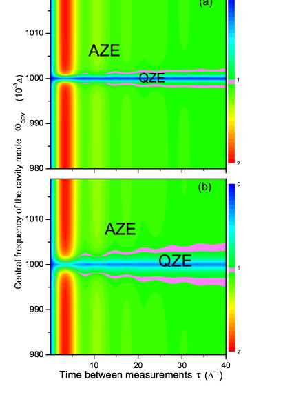
Figure 7: (Color online) The qubit-cavity coupling is $g=10^{-3}\Delta$. The other caption is the same as Fig. 6.

In Figs. 6 and 7, we plot the normalized effective decay rate, when the cavity bath and the low-frequency qubit spontaneous dissipation bath coexist, versus the time interval $\tau$ between measurements in the regime of strong ($g=10^{-2}\Delta$) and weak ($g=10^{-3}\Delta$) cavity-qubit coupling with the cavity central frequency around the qubit energy-level-spacing $\Delta.$ Figures 6(a) and (b) correspond to the cavity quality factor $Q=10^{4}$ and $Q=2\times 10^{3}$, respectively. From Fig. 6, we see that for a strong qubit-cavity coupling, by modulating the cavity central frequency from in-resonance to off-resonance with the qubit energy-level-spacing, the normalized effective decay rate grows and becomes larger than $1,$ which clearly displays the transition from the QZE to the AZE. Comparing Figs. 6(a) and (b), as the width $\lambda$ of the cavity frequency decreases (or the quality factor $Q=\omega_{\mathrm{cav}}/\lambda$ increases), the region of the cavity frequency for the QZE becomes narrower. For example, Table I presents the normalized effective decay rate $\gamma(\tau)/\gamma_{0}$ for two quality factors $Q$ and different central frequencies $\omega_{\mathrm{cav}}$ of the cavity, when $\tau=5\;\Delta^{-1}$.

Table 1: The normalized effective decay rate $\gamma(\tau)/\gamma_{0}$ of the qubit for two quality factors $Q$ when $\tau=5\;\Delta^{-1}$, in the presence of both the cavity bath and the low-frequency qubit’s intrinsic bath.

Cavity quality factor	Central frequency of the cavity
	$0.98\Delta$	$\;0.99\Delta$	$0.999\Delta$	$\Delta$	$1.001\Delta$	$1.01\Delta$	$1.02\Delta$
$Q=10^{4}$	1.994	1.784	0.122	0.001	0.122	1.777	1.979
$Q=2\times 10^{3}$	1.727	1.149	0.032	0.006	0.032	1.145	1.714

For weak qubit-cavity coupling in Fig. 7, only in the short-time regime (about $2\Delta^{-1}<\tau<6\Delta^{-1}$), the normalized effective decay rate of the qubit shows obviously the transition from the QZE to the AZE. When the measurement interval $\tau$ increases to $\tau>10\Delta^{-1}$, although the transition still exists, $\gamma(\tau)/\gamma_{0}$ for the AZE is slightly larger than 1, which is mainly in the region between $1.0$ and $1.1.$

In Figs. 6 and 7, there appear distinct oscillations in the qubit’s QZE-AZE transition processes. From the results of Ref. [arkiv, ], we have known that the AZE always occurs for a qubit in the low-frequency bath. While, for a qubit in the cavity bath, the transition from QZE to AZE takes place by varying the cavity frequency. These oscillations in Figs. 6-7 come from the different impacts of the cavity-bath and the low-frequency bath on the qubit’s measurement dynamics.

V.3 Coexistence of the cavity bath and the Ohmic qubit spontaneous dissipation bath

Figure 8: (Color online) Contour plots of the normalized effective decay rate $\gamma(\tau)/\gamma_{0}$ in the presence of both: the cavity bath and the Ohmic qubit’s intrinsic bath. The interaction strength $\alpha_{\mathrm{Ohm}}=10^{-4}$, between the qubit and the qubit’s intrinsic bath. Also the qubit-cavity coupling $g=10^{-2}\Delta$. (a) The cavity quality factor of the cavity $Q=10^{4}.$ (b) The cavity quality factor $Q=2\times 10^{3}.$ The region $1\leq\gamma(\tau)/\gamma_{0}\leq 1.05$ is shown as light magenta. The QZE region corresponds to $\gamma(\tau)/\gamma_{0}<1$. The AZE region is the rest, when $\gamma(\tau)/\gamma_{0}>1$. Evidently, a transition from the  QZE to the AZE is observed by varying the central frequency $\omega_{\mathrm{cav}}$ of the cavity mode at finite $\tau$.

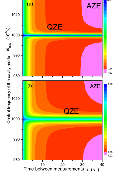
Figure 9: (Color online) The qubit-cavity coupling $g=10^{-3}\Delta$. The other caption is the same as Fig. 8

In Figs. 8 and 9, we show the normalized effective decay rate $\gamma(\tau)/\gamma_{0}$ in the presence of both the Ohmic intrinsic bath and cavity bath. Comparing Figs. 8 with 6, we find that for the strong qubit-cavity coupling $g=10^{-2}\Delta,$ the time interval $\tau$ for the QZE increases in the short-time region. In the long-time region, the features of Figs. 6 and 8 are almost identical. From Fig. 9 we can see that in the short-time region, ($0<\tau<30\Delta^{-1})$, only the QZE exists, regardless of the central frequency of cavity. For $\tau>30\Delta^{-1},$ the normalized effective decay rate $\gamma/\gamma_{0}$ for the AZE is in the small region of $1.0\sim 1.02$, which is not conducive to observe the transition from the QZE to the AZE.

VI Summary

We investigated the QZE and AZE of a qubit in a cavity when both the cavity bath and the qubit’s intrinsic bath (either low-frequency or Ohmic bath) are simultaneously present. We find that in the case of strong qubit-cavity coupling, modulating the cavity central frequency from on-resonance ($\omega_{\mathrm{cav}}=\Delta)$ to off-resonance ($\omega_{\mathrm{cav}}$ larger or smaller than $\Delta)$ with the qubit energy-level-spacing, the transition from the QZE to the AZE occurs. Thus, our results provide a proposal to observe the QZE and the AZE in the qubit-cavity system.

Acknowledgements

We thank A. G.  Kofman for comments on the manuscript. FN acknowledges partial support from DARPA, AFOSR, the National Security Agency (NSA), Laboratory for Physical Sciences (LPS), Army Research Office (USARO), National Science Foundation (NSF) under Grant No. 0726909, JSPS-RFBR under Contract No. 09-02-92114, MEXT Kakenhi on Quantum Cybernetics, and FIRST (Funding Program for Innovative R&D on S&T). X.-F. Cao acknowledges support from the National Natural Science Foundation of China under Grant No. 10904126 and Fujian Province Natural Science Foundation under Grant No. 2009J05014.

——————–

References

- (1) W. M. Itano, D. J. Heinzen, J. J. Bollinger, and D. J. Wineland , Phys. Rev. A 41, 2295 (1990).
- (2) A. Peres and A. Ron, Phys. Rev. A 42, 5720 (1990).
- (3) E. Block and P. R. Berman, Phys. Rev. A 44, 1466 (1991).
- (4) M. Namiki, S. Pascazio and H. Nakazato, Decoherence and Quantum measurements (World Scientific, Singapore, 1997).
- (5) A. G. Kofman and G. Kurizki, Nature 405, 546 (2000).
- (6) P. Facchi, H. Nakazato, and S. Pascazio, Phys. Rev. Lett. 86, 2699(2001).
- (7) Q. Ai, D. Xu, S. Yi, A. G. Kofman, C. P. Sun, F. Nori, arXiv:1007.4859 (2010).
- (8) M. C. Fischer, B. Gutiérrez-Medina, and M. G. Raizen, Phys. Rev. Lett. 87, 040402 (2001).
- (9) S. Maniscalco, J. Piilo, and K.-A. Suominen, Phys. Rev. Lett. 97, 130402 (2006).
- (10) H. Park, J. Park, A. K. L. Lim, E. H. Anderson, A. P. Alivisatos, and P. L. McEuen, Nature (London) 407, 57 (2000).
- (11) C. J. Myatt, B. E. King, Q. A. Turchette, C. A. Sackett, D. Kielpinski, W. M. Itano, C. Monroe, and D. J. Wineland, Nature (London) 403, 269 (2000).
- (12) P.-W. Chen, D.-B. Tsai and P. Bennett, Phys. Rev. B 81, 115307 (2010).
- (13) I. Lizuain, J. Casanova, J. J. Carcía-Ripoll, J. G. Muga, and E. Solano, Phys. Rev. A 81, 062131 (2010).
- (14) A. G. Kofman and G. Kurizki, Phys. Rev. A 54, R3750 (1996).
- (15) C. Search and P. R. Berman, Phys. Rev. Lett. 85, 2272 (2000).
- (16) J. Bernu, S. Deleglise, C. Sayrin, S. Kuhr, I. Dotsenko, M. Brune, J. M. Raimond, and S. Haroche, Phys. Rev. Lett. 101, 180402 (2008).
- (17) J. Q. You and F. Nori, Phys. Rev. B 68, 064509 (2003).
- (18) A. Blais, R.-S. Huang, A. Wallraff, S. M. Girvin, and R. J. Schoelkopf, Phys. Rev. A 69, 062320 (2004).
- (19) J. R. Johansson, G. Johansson, C. M. Wilson, and F. Nori, Phys. Rev. Lett. 103, 147003 (2009); Phys. Rev. A 82, 052509 (2010).
- (20) J.-Q. Liao, Z. R. Gong, L. Zhou, Y.-X. Liu, C. P. Sun, and F. Nori, Phys. Rev. A 81, 042304 (2010).
- (21) M. Wallquist, V. S. Shumeiko, and G. Wendin, Phys. Rev. B 74, 224506 (2006).
- (22) M. Sandberg, C. M. Wilson, F. Persson, T. Bauch, G. Johansson, V. Shumeiko, T. Duty, and P. Delsing, Appl. Phys. Lett. 92, 203501 (2008).
- (23) T. Yamamoto, K. Inomata, M. Watanabe, K. Matsuba, T. Miyazaki, W. D. Oliver, Y. Nakamura, and J. S. Tsai, Appl. Phys. Lett. 93, 042510 (2008).
- (24) M. A. Castellanos-Beltran, K. D. Irwin, G. C. Hilton, L. R. Vale, and K. W. Lehnert, Nature Phys. 4, 929 (2008).
- (25) M. A. Castellanos-Beltran and K. W. Lehnert, Appl. Phys. Lett. 91, 083509 (2007).
- (26) H. Zheng, S. Y. Zhu, and M. S. Zubairy, Phys. Rev. Lett. 101, 200404 (2008).
- (27) Q. Ai, Y. Li, H. Zheng, and C. P. Sun, Phys. Rev. A 81, 042116 (2010).
- (28) S. De Liberato, D. Gerace, I. Carusotto, and C. Ciuti, Phys. Rev. A 80, 053810 (2009).
- (29) Y. B. Gao, Y. D. Wang, and C. P. Sun, Phys. Rev. A 71, 032302 (2005).
- (30) L. Mazzola, S. Maniscalco, J. Piilo, K.-A. Suominen, and B. M. Garraway, Phys. Rev. A 79, 042302 (2009).
- (31) H. J. Carmichael, R. J. Brecha, M. G. Raizen, H. J. Kimble and P. R. Rice, Phys. Rev. A 40, 5516 (1989).
- (32) L. Zhou, S. Yang, Y.-X. Liu, C. P. Sun and F. Nori, Phys. Rev. A 80, 062109 (2009).
- (33) A. Wallraff, D. I. Schuster, A. Blais, L. Frunzio, R.-S. Huang, J. Majer, S. Kumar, S. M. Girvin, and R. J. Schoelkopf, Nature 431, 162 (2004).
- (34) G. Gunter, A. A. Anappara, J. Hees, A. Sell, G. Biasiol, L. Sorba, S. De Liberato, C. Ciuti, A. Tredicucci, A. Leitenstorfer and R. Huber, Nature 458, 178 (2009); A. A. Anappara, S. De Liberato, A. Tredicucci, C. Ciuti, G. Biasiol, L. Sorba, and F. Beltram, Phys. Rev. B 79, 201303(R) (2009).
- (35) T. Niemczyk, F. Deppe, H. Huebl, E. P. Menzel, F. Hocke, M. J. Schwarz, J. J. Garcia-Ripoll, D. Zueco, T. Hümmer, E. Solano, A. Marx and R. Gross, Nat. Phys. 6, 772 (2010).
- (36) X. Cao, J. Q. You, H. Zheng, A. G. Kofman and F. Nori, Phys. Rev. A 82, 022119 (2010).