Arrayed and checkerboard optical waveguides controlled by the electromagnetically-induced transparency

Abstract

We introduce two models of quasi-discrete optical systems: an array of waveguides doped by four-level N-type atoms, and a nonlinear checkerboard pattern, formed by doping with three-level atoms of the $\Lambda$-type. The dopant atoms are driven by external fields, to induce the effect of the electromagnetically-induced transparency (EIT). These active systems offer advantages and addition degrees of freedom, in comparison with ordinary passive waveguiding systems. In the array of active waveguides, the driving field may adjust linear and nonlinear propagation regimes for a probe signal. The nonlinear checkerboard system supports the transmission of stable spatial solitons and their ”fuzzy” counterparts, straight or oblique.

I INTRODUCTION

The transmission of light in discrete arrays of evanescently coupled waveguides is a topic of great interest in optics. The arrays are prime examples of systems in which the discrete optical dynamics can be observed and investigated Lederer (2008). Optical fields propagating in such settings exhibit a great number of novel phenomena Lederer (2008); Kartashov (2009); Schwartz (2007). However, traditional coupled arrays or lattices, such as arrays of waveguides made of AlGaAs yaron (1998) or periodically poled lithium niobate (PPLN) Iwanow (2004), virtual lattices created in photorefractive crystals (PhCs) Fleischer2 (2003) and liquid crystals Fratalocchi (2006) by means of the optical induction, etc., are built of passive ingredients.

On the other hand, it is well known that active elements, such as atoms with a near-resonant transition frequency, may lend the medium a number of specific optical characteristics, such as strong dispersion, a complex dielectric constant, and the strong variation of the dispersion relation near the resonance. Therefore, waveguide arrays made of active elements may offer low thresholds, in comparison with their passive counterparts, and possibilities for the “management” of their waveguiding characteristics. In the 1D (one-dimensional) case, active discrete systems were previously studied in detail in the form of resonantly-absorbing Bragg reflectors (RABRs) Kurizki (1998), which are used to demonstrate optical switching Prineas (2002), storage JYZhou (2005), and nonlinear conversion JTLi (2006).

Recently, a 2D (two-dimensional) “imaginary-part photonic crystal” (IPPhC, i.e., a medium with a periodic variation of the imaginary part of the refractive index) is realized by means of the techniques of multi-beam-interference holography, lithography and back-filling juntaoli (2010), which allows one to create a spatially-structured distribution of the active material. For example, active substance Rhodamine B can be doped into the homogeneous SU8 background to form an IPPhC. In this structure, the real part of the refractive index is constant if the probe wavelength is far detuned from the resonance. However, the imaginary part of refractive index affects the real part, which becomes a conspicuous effect close to the resonance. Thus, in the vicinity the absorption window, the IPPhC also acts as a traditional PhC. Very recently, a laser system in a medium featuring a periodic distribution of loss, which is akin to IPPhC, is demonstrated in the experiment WXYYYL (2010).

In this work we propose two new varieties of active light-guiding systems. In Section II, we show that the introduction of an active material into the PhC provides for a way to create active structures in the form of a coupled waveguide arrays. The difference of this system from the RABR is that guides light not across the periodic structure, but rather along it. In Section III, we introduce a checkerboard system, which is built of alternating linear and the nonlinear square cells in the $x$-$z$ plane. These systems may be controlled (“managed”) via the effect of the electromagnetic-induced transparency (EIT).

II Waveguiding arrays controlled by the electromagnetically-induced transparency

In this section we consider the possibility to use N-type near-resonant four-level atoms as the active dopant. The respective scheme of the energy levels is shown in FIG. 1(a), where $|1\rangle$ and $|2\rangle$ are the ground and a metastable states, respectively. These two states have the same parity of their wave functions, which is opposite to that of states $|3\rangle$ and $|4\rangle$.

As a part of the scheme, we assume that a weak probe wave, $E_{P}$, with Rabi frequency $\Omega_{P}=\wp_{31}E_{P}/\hbar$ is acting on transition $|1\rangle\rightarrow|3\rangle$, with single-photon detuning $\Delta_{1}$. Here $\wp_{31}$ (which is assumed real) is the matrix element of the dipole transition between $|1\rangle$ and $|3\rangle$ . Further, a traveling-wave field with Rabi frequency $\Omega_{C}$ drives the atomic transition $|2\rangle\rightarrow|3\rangle$ with detuning $\Delta_{C}=\Delta_{1}$, hence the two-photon detuning is given by $\delta=\Delta_{1}-\Delta_{C}\equiv 0$. As another ingredient of the EIT scheme, an optical-induction field with Rabi frequency $\Omega_{S}$ induces transition $|2\rangle\rightarrow|4\rangle$, with detuning $\Delta_{2}$. The decay rate for level $|n\rangle$ is $\gamma_{n}$. Here we neglect $\gamma_{1}$ and $\gamma_{2}$, and assume $\gamma_{3}\approx\gamma_{4}\equiv\gamma$.

The Hamiltonian of the system is:

$$H =\sum^{4}_{l=1}\hbar\omega_{l}|l\rangle\langle l|-{1\over 2}[\Omega_{P}e^{-i\omega_{P}t}|3\rangle\langle 1|+$$ (1)

$$\Omega_{C}e^{-i\omega_{C}t}|3\rangle\langle 2|+\Omega_{S}e^{-i\omega_{S}t}|4\rangle\langle 2|+H.C].$$

where $\omega_{l}$ is the eigenfrequency of the l-th level. The EIT effect means that, when the probe is exactly at the two-photon resonance ($\delta=0$), and the atoms are prepared in the ground state, the linear absorption of the probe vanishes, irrespective of the single-photon detuning Fleischhauer (2005).

The quasi-discrete system, which is introduced in this section, is illustrated by panel (b1) in FIG. 1, which shows the distribution of the concentration of the active component in the 1D case. The transverse width of the waveguide is $d_{1}$, the interval between the waveguides is $d_{2}$, and $N_{0}$ is the density of the N-type atoms inside the waveguides. Coefficients are chosen as per experimental in the case of Y₂SiO₅ doped with Pr³⁺ (Pr:YSO) Ham (1997): the density of active atoms inside the waveguides is $N_{0}=1.0\times 10^{18}$cm³ (which corresponds to the dopant concentration $\approx$0.1%), $\wp_{31}=1.18\times 10^{-32}$C$\cdot$m, and $\gamma=30$ kHz, the probe wavelength being 605 nm. Linear and the nonlinear properties of this system are detailed below.

(1) Linear properties of the system

If we set $\Delta_{1}=0$ and assume $\Delta_{2}\gg\Omega_{C},\gamma$ , then the absorption of the probe can be neglected. One can easily find the one-step steady-state solution for the density-matrix element of the transition between $|1\rangle$ and $|3\rangle$ , cf. Ref. Lukin (2002):

$$\rho_{31}={|\Omega_{S}|^{2}\over 2\Delta_{2}|\Omega_{C}|^{2}}\Omega_{P}.$$ (2)

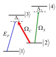
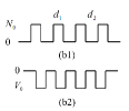
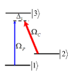
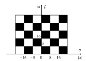
Figure 1: (Color online) (a) The energy-level diagram of the N-type atom. (b1) The structure of the active waveguide array: the transverse width of the waveguide is $d_{1}$ , the interval between the waveguides is $d_{2}$, and the density of the active atoms in the waveguide is $N_{0}$ . (b2) The respective effective periodic potential with $V_{0}=-N_{0}\wp^{2}_{31}|\Omega_{S}|^{2}/2\epsilon_{0}\hbar\Delta_{2}|\Omega_{C}|^{2}$ . (c) The energy-level diagram of the $\Lambda$-type atom. (d) The checkerboard system: black and white square cells depict areas which are, respectively, doped with the active material, or are left undoped.

Therefore, the contribution of the resonant atoms to the polarization experienced by the probe is $\mathscr{P}=2N\wp_{31}\rho_{31}$, cf. Ref. Scully (1997) (recall $N$ is the dopant density). The (1+1)D paraxial propagation equation for the slowly varying envelope of the probe field, $E_{P}$, is

$$2ik_{P}{\partial\over\partial z}E_{P}=-{\partial^{2}\over\partial x^{2}}E_{P}-{k^{2}_{P}\over\epsilon_{0}}\mathscr{P},$$ (3)

where $k_{P}=2\pi n/\lambda_{P}$ is the wavenumber of the probe, and $n$ the background refractive index. The substitution of Eq. (2) into the last term of Eq. (3) yields a scaled linear Schrödinger equation,

$$i{\partial\over\partial\zeta}U=-{1\over 2}{\partial^{2}\over\partial\eta^{2}}U+V(\eta)U,$$ (4)

where $\zeta=k_{p}z$, $\eta=k_{p}x$, $U=\Omega_{P}/\gamma$, and the effective potential,

$$V(\eta)=-{\wp^{2}_{31}\over 2\epsilon_{0}\hbar\Delta_{2}}{|\Omega_{S}|^{2}\over|\Omega_{C}|^{2}}N(\eta).$$ (5)

is induced by the concentration distribution $N(\eta)$ , as shown in panel (b1) of FIG. 1. This potential is induced by the giant Kerr effect controlled by the Rabi frequency $\Omega_{S}$ Schmidt (1996). In fact, this potential emulates a difference in the local refractive index contrast between the active (doped) and passive (undoped) regions. For $\Delta_{2}>0$ (here, we choose $\Delta_{2}=100\gamma$), the shape the potential is shown in panel (b2) of FIG. 1, which is similar to the Kronig-Penney potentials corresponding to the tight-binding model in solid-state physics Kittel (1995). The depth of local wells in the periodic potential is defined by the intensity ratio, $|\Omega_{S}|^{2}/|\Omega_{C}|^{2}$, the corresponding refractive-index contrast between the active and passive regions being $\Delta n=\wp^{2}_{31}N_{0}|\Omega_{S}|^{2}/2\epsilon_{0}\hbar\Delta_{2}|\Omega_{C}|^{2}$

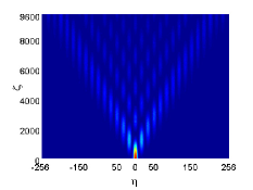
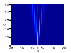
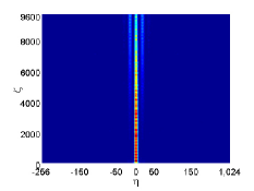
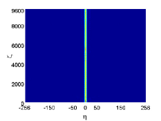
Figure 2: (Color online) Simulations of the linear transmission of light in the arrays of active waveguides. Here, we chose $d_{1}=d_{2}=8$, $\Omega_{C}=2\gamma$ and $\Delta_{2}=100\gamma$. The incident beam (at $\zeta=0$) is $U=A_{0}\exp(-\eta^{2}/d^{2}_{1})$ with $A_{0}=0.07$. (a) $|\Omega_{S}|^{2}=0.036|\Omega_{C}|^{2}$ (i.e., $\Delta n=0.09$). (b) $|\Omega_{S}|^{2}=0.064|\Omega_{C}|^{2}$ (i.e., $\Delta n=0.16$). (c) $|\Omega_{S}|^{2}=0.100|\Omega_{C}|^{2}$ (i.e., $\Delta n=0.25$). (d) $|\Omega_{S}|^{2}=0.144|\Omega_{C}|^{2}$ (i.e., $\Delta n=0.36$).

Figure 2 displays the propagation of the probe in such a system at different values of $|\Omega_{S}|^{2}/|\Omega_{C}|^{2}$ (i.e. different values of $\Delta n$), produced by numerical simulations of Eq. (4). This figure demonstrates that the quasi-discrete diffraction naturally gets suppressed when the depth of the potential, i.e., $|\Omega_{S}|^{2}/|\Omega_{C}|^{2}$ or $\Delta n$, increases, resulting in a reduced coupling between local waveguides. Thus, the diffraction in the present setting may be efficiently controlled by varying the magnitude of $|\Omega_{S}|^{2}/|\Omega_{C}|^{2}$.

(2) Nonlinear properties of the system

If both detunings satisfy conditions $\Delta_{1},\Delta_{2}\gg\Omega_{C},\gamma$, then the absorption of the probe (the losses) may be neglected. Moreover $\Delta_{1}\neq 0$ produces an enhanced Kerr nonlinearity XiaoMin (2001), provided that the density matrix element $\rho_{31}$, which accounts for transitions between $|1\rangle$ and $|3\rangle$, is taken into regard, to describe the third-order effect. The steady-state solution for this matrix element can be obtained in the following from, cf. Ref. lyy (2010):

$$\rho_{31}=\rho^{(1)}_{31}+\rho^{(2)}_{31}+\rho^{(3)}_{31}\approx{|\Omega_{S}|^{2}\over 2\Delta_{2}|\Omega_{C}|^{2}}\Omega_{P}-{|\Omega_{P}|^{2}\over 2\Delta_{1}|\Omega_{C}|^{2}}\Omega_{P}$$ (6)

With regard to this result and the above definition, $U=\Omega_{P}/\gamma$, Eq. (3) changes its form into that of the standard nonlinear Schrödinger (NLS) equation Kevekidis (2009):

$$i{\partial\over\partial\zeta}U=-{1\over 2}{\partial^{2}\over\partial\eta^{2}}U+V(\eta)U+\kappa(\eta)|U|^{2}U,$$ (7)

where the effective nonlinear coefficient is

$$\kappa(\eta)={\wp^{2}_{31}\over 2\epsilon_{0}\hbar\Delta_{1}(|\Omega_{C}|^{2}/\gamma^{2})}N(\eta)$$ (8)

Thus, $E_{P}$ is affected by the modifications of the refractive index of two types: (1) a periodic change of the linear index induced by $\Omega_{S}$ via the giant Kerr effect; (2) the nonlinear change under the action of $E_{P}$ itself, via the enhanced self-Kerr effect. The sign of detuning $\Delta_{1}$ determines whether the latter effect gives rise to the self-focusing ($\Delta_{1}<0$) or self-defocusing ($\Delta_{1}>0$) sign of the nonlinearity. When the tunneling coupling between adjacent waveguides is balanced by the nonlinearity, quasi-discrete solitons Mayteevarunyoo (2008) can be formed in this system, which is similar to those in the traditional coupled arrays made of passive materials Kominis (2006).

III Solitons in the checkerboard system controlled by the electromagnetically-induced transparency

In this section, we assume that the active material is doped periodically in both the transverse and propagation directions (i.e., along the x and z axes, respectively). The corresponding density distribution of the active material is $N(x,z)=N_{0}R(x,z)$, where $R(x,z)$ is a dimensionless structural function of the distribution. Here, we adopt for $R(x,z)$ the form checkerboard form depicted in FIG. 1(d). The white cells, with $R(x,z)=0$ , are areas which are not subject to the doping, while black cells, with $R(x,z)=1$ , depict areas doped by the active material.

Note that the formation of 2D spatial solitons in the checkerboard-shaped linear potential was considered in Ref. Malomed (2007), assuming that the probe beam was shone along the uniform direction in the bulk medium equipped with the transverse checkerboard structure. Here, the difference is that the modulation is applied to the nonlinear term, and light propagated across the structure.

If we turn off the control field $\Omega_{S}$, the four-level N-type atomic configuration reduces to the three-level one of the $\Lambda$-type, see FIG. 1(c). In this case, the linear-refractive-index contrast between the active and the passive areas vanishes, which leaves only the nonlinearity modulation in action.

Again assuming that the detuning is much larger than the decay rate, $\Delta_{1}\gg\gamma$ , the absorption of the probe may be ignored as before. Accordingly, in the present setting Eq. (6) is rewritten as:

$$\rho_{31}=\rho^{(1)}_{31}+\rho^{(2)}_{31}+\rho^{(3)}_{31}\approx-{|\Omega_{P}|^{2}\over 2\Delta_{1}|\Omega_{C}|^{2}}\Omega_{P}$$ (9)

and Eq. (3) changes into

$$i{\partial\over\partial\zeta}U=-{1\over 2}{\partial^{2}\over\partial\eta^{2}}U+\kappa(\eta,\zeta)|U|^{2}U,$$ (10)

where we define

$$\kappa(\eta,\zeta)={\wp^{2}_{31}N_{0}\over 2\epsilon_{0}\hbar\Delta_{1}(|\Omega_{C}|^{2}/\gamma^{2})}R(\eta,\zeta)\equiv\kappa_{0}R(\eta,\zeta)$$ (11)

Therefore, the white and black cells, with $\kappa(\eta,\zeta)=0$, and $\kappa(\eta,\zeta)=\kappa_{0}$, act as linear and nonlinear elements, respectively.

The periodic modulation of the nonlinearity in Eq. (10) places this equation into the broad class of models with nonlinear lattices (see original works Sakaguchi (2005) and review Kartashov (2011)). However, the present checkerboard pattern of the modulation in the longitudinal and transverse direction was not studied in previous works. More general patterns, that should be studied separately, may be represented by arrays of isolated black squares set against the white background, or vice versa.

Below, we choose values $\Delta_{1}=-100\gamma$, $\Omega_{C}=0.5\gamma$, with the other parameters taken as before. This yields the nonlinearity-modulation amplitude $\kappa_{0}=-10$ . The probe field is launched at $\zeta=0$ as a Gaussian

$$U(\eta,0)=A\exp[-(\eta-\alpha)^{2}/W^{2}],$$ (12)

with the central point at $\eta=\alpha$. For the simulations, we take the checkerboard with squares of size $8\times 8$, as shown in FIG. 1(d).

The simulations of the evolution of the Gaussian in the framework of Eq. (10) were carried out by means of the split-step Fourier method. First, we chose the amplitude and width of Gaussian (12) as, $A$=0.075, 0.065, 0.055 and $W$=8, with the center placed at the mid-point of the nonlinear cell ($\alpha=4$). Results of the simulations are displayed in FIG. 3(a)-(c). In particular, FIG. 3(a) shows that the probe field with $A$=0.075 propagates without decay and distortion over the distance longer than $z=100\times W^{2}$, i.e., $\sim$100 diffraction lengths. This dynamical regime may be naturally identified as a stable soliton. On the other hand, in FIG. 3 (b), with the Gaussian’s amplitude $A$=0.065, the probe field forms a fuzzy beam, which, nevertheless, avoids decay over the distance exceeding $z=100\times W^{2}$.

However, for $A$=0.055, FIG. 3(c) demonstrates that the input cannot form a robust beam and rapidly decays. Therefore, there must be internal borders (i.e. thresholds) separating the stable solitons, fuzzy beams, and decaying ones, in the plane of the width and amplitude of the Gaussian inputs. These borders are plotted in FIG. 3(d).

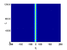
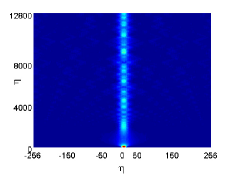
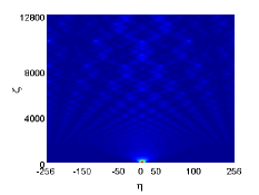
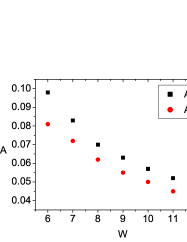
Figure 3: (Color online) Simulations of the evolution of the Gaussian input probe with width $W=8$ in the checkerboard model. (a) With amplitude $A$=0.075, the probe propagates in a stable fashion over the distance of $L=200\times W^{2}=12800$. This beam may be called a stable soliton. (b) With $A=0.065$, the probe propagates, keeping a fuzzy shape, still featuring robustness against the diffractive spreading-out. (c) With $A=0.055$, the probe quickly spreads out. (d) In the plane of the width and amplitude if the input Gaussian, $A^{1}_{C}(W)$ is the border between the stable and fuzzy beams, while $A^{2}_{C}(W)$ is the border between the fuzzy but robust beams and decaying inputs.

Further simulations, displayed in FIG. 4(a), show that stable straight solitons can be formed as well if the Gaussian is launched at the midpoint of the linear cell. However, if the center of the Gaussian does not coincide with the center of the linear or nonlinear cell, the propagation of the soliton beam becomes oblique, see an example in FIG. 4(b).

It may be interesting to consider the oblique propagation of beams across the checkerboard, induced by the application of a lateral kick to the input. Another issue of obvious interest is the interaction of beams in this setting. These generalizations will be reported elsewhere.

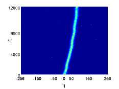
Figure 4: (Color online) (a) The probe with parameters $A=0.075$, $W=8$, and $\alpha=-4$ is launched at the mid-point of the linear cell. The probe propagates in a stable fashion over distance $L=200\times W^{2}=12800$, therefore it is categorized as a stable soliton. (b) The probe with $A=0.075$, $W=8$, $\alpha=0$ propagate obliquely if it is launched off the mid-point of a linear or nonlinear cell.

IV CONCLUSION

In this work, we have proposed a method for building systems of coupled active waveguides, and also a new system with the checkerboard pattern of the modulation of the nonlinearity coefficient. These settings can be created using the appropriate doping patterns of the N-type four-level and $\Lambda$-type three-level resonant atoms, respectively, and driving them by means of the EIT mechanism. Such active systems offer certain advantages, admitting more possibilities for the design and management, in comparison to the passive media. Firstly, the nonlinearity in the active systems can be switched via the sign of detuning $\Delta_{1}$: the incident beam with $\Delta_{1}<0$ and $\Delta_{1}>0$ will experience the action of the self-focusing and self-defocusing nonlinearity, respectively. Next, it is well known that the EIT may be efficiently applied to few-photon settings, especially in the nonlinear regimen Fleischhauer (2005); T-Hong (2003). Therefore, the systems introduced here may, in principle, offer an advantage for handling quantum and non-classical light beams, composed of few photons. Further, it is well known that the group velocity of the probe can be coherent controlled lyy3 (2009) and tuned to a very small value under the action of the EIT Hau (1999), which implies that the probe signal in this system can be trapped in the from of the slow light. Thus, various applications of the EIT, such as dark-state polaritons Lukin (2000), the few-photon four-wave mixing Fleischhauer (2002), ultra-weak and ultraslow light liyongyao (2010), etc., may be realized in the systems proposed here. Furthermore, using properly designed holographic patterns, various complex spatial structures of the distribution of the dopant concentration can be photoinduced in the 2D geometry, such as quasi-crystals Freeedman (2006), honeycomb lattices Peleg (2007), defect lattices liyongyao3 (2009), ring lattices WXS (2006), etc., in addition to the simplest checkerboard patterns analyzed herein. Such 2D structures may have their own spectrum of potential applications.