Homogenization of spectral problem on Riemannian manifold consisting of two domains connected by many tubes

Abstract

The paper deals with the asymptotic behavior as ${\varepsilon}\to 0$ of the spectrum of Laplace-Beltrami operator $\Delta^{\varepsilon}$ on the Riemannian manifold $M^{\varepsilon}$ ($\mathrm{\dim}M^{\varepsilon}=N\geq 2$) depending on a small parameter ${\varepsilon}>0$. $M^{\varepsilon}$ consists of two perforated domains which are connected by array of tubes of the length $q^{\varepsilon}$. Each perforated domain is obtained by removing from the fix domain $\Omega\subset\mathbb{R}^{N}$ the system of ${\varepsilon}$-periodically distributed balls of the radius $d^{\varepsilon}=\bar{o}({\varepsilon})$. We obtain a variety of homogenized spectral problems in $\Omega$, their type depends on some relations between ${\varepsilon}$, $d^{\varepsilon}$ and $q^{\varepsilon}$. In particular if the limits $\lim\limits_{{\varepsilon}\to 0}q^{\varepsilon}$ and $\lim\limits_{{\varepsilon}\to 0}\displaystyle{(d^{\varepsilon})^{N-1}q^{\varepsilon}{\varepsilon}^{-N}}$ are positive then the homogenized spectral problem contains the spectral parameter in a nonlinear manner, and its spectrum has a sequence of accumulation points.

Introduction

The aim of this paper is to study the asymptotic behavior as ${\varepsilon}\to 0$ of the spectrum of Laplace-Beltrami operator $\Delta^{\varepsilon}$ (with Dirichlet boundary conditions) on the $N$-dimensional Riemannian manifold $M^{\varepsilon}$ $(N\geq 2)$ depending on small parameter ${\varepsilon}>0$. The manifold $M^{\varepsilon}$ is embedded in $\mathbb{R}^{N+1}$. It is constructed in the following way. Let $\Omega$ be a bounded smooth domain in $\mathbb{R}^{N}$ and let $\left\{D_{i}^{\varepsilon}\right\}_{i}$ be a system of disjoint balls (”holes”) of the radius $d^{\varepsilon}$ distributed ${\varepsilon}$-periodically in $\Omega$. Denote $\Omega^{\varepsilon}=\Omega\setminus\bigcup\limits_{i}D_{i}^{\varepsilon}$. Then $M^{\varepsilon}$ consists of two parallel perforated sets $\Omega_{1}^{\varepsilon}$ and $\Omega_{2}^{\varepsilon}$ (each of them is the copy of $\Omega^{\varepsilon}$) and the set $\left\{G_{i}^{\varepsilon}\right\}_{i}$ of cylinders of the length $q^{\varepsilon}$ and the radius $d^{\varepsilon}$ (the cylinder $G_{i}^{\varepsilon}$ connects the boundaries of $i$-th holes in $\Omega_{1}^{\varepsilon}$ and $\Omega_{2}^{\varepsilon}$):

$$M^{\varepsilon}=\Omega_{1}^{\varepsilon}\cup\left(\bigcup\limits_{i}G_{i}^{\varepsilon}\right)\cup\Omega_{2}^{\varepsilon}.$$

The manifold $M^{\varepsilon}$ is presented on Fig.1. We equip $M^{\varepsilon}$ by Riemannian metric $g^{\varepsilon}$ which is induced on $M^{\varepsilon}$ by Euclidean metric in $\mathbb{R}^{N+1}$. More precise description of $M^{\varepsilon}$ will be specified later in Section 1.

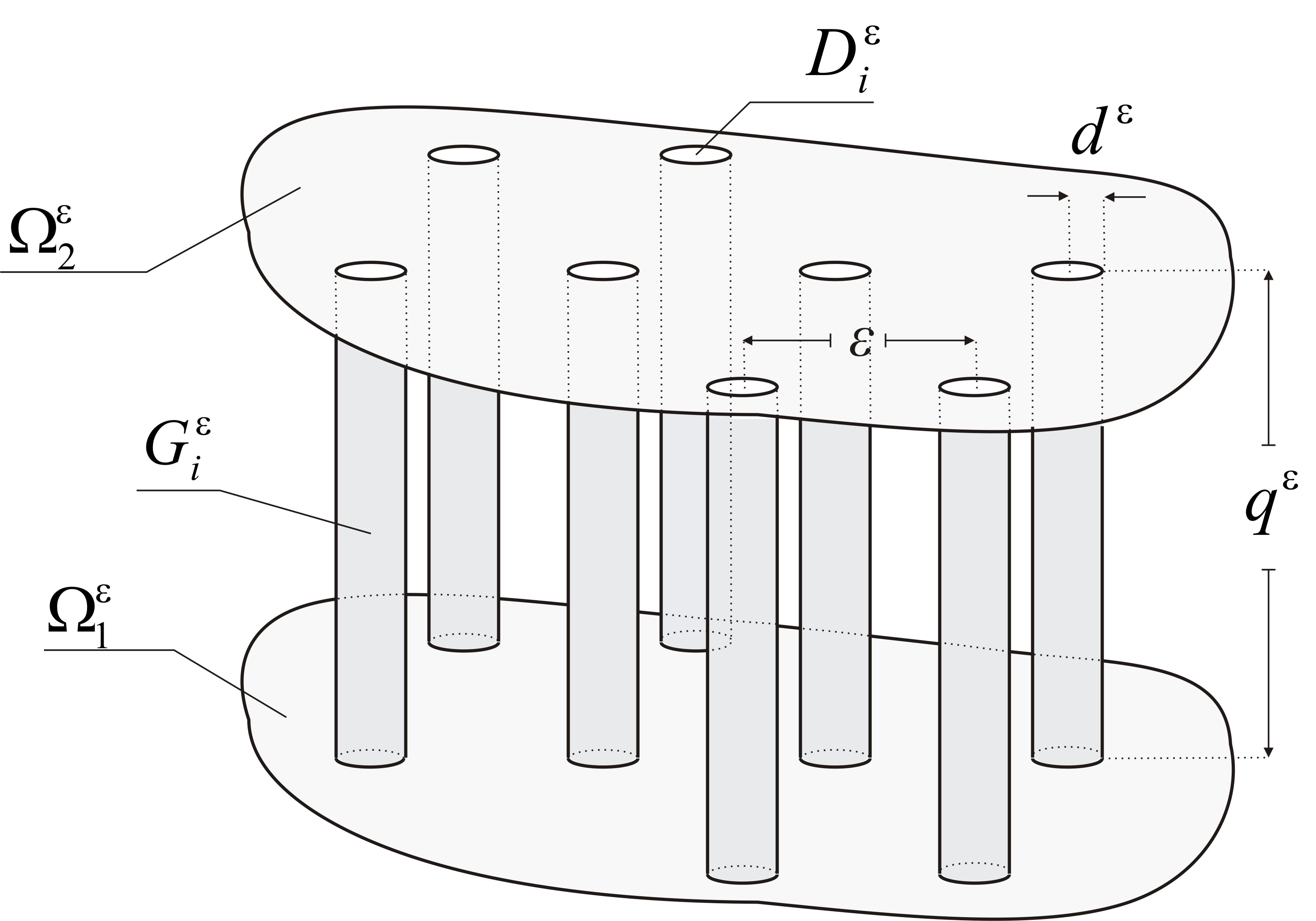
Figure 1: The manifold $M^{\varepsilon}$

We denote by $\sigma(-\Delta^{\varepsilon})=\{\lambda^{\varepsilon}_{m}\}_{m\in\mathbb{N}}$ the sequence of eigenvalues of $-\Delta^{\varepsilon}$ (here they are renumbered in the increasing order and repeated according to their multiplicity). By $\left\{u^{\varepsilon}_{m}\right\}_{m\in\mathbb{N}}$ we denote the system of corresponding eigenfunctions that are chosen orthonormal in ${L_{2}(M^{\varepsilon})}$.

Our goal is to find the homogenized spectral problem in $\Omega$ whose spectrum is a limit of $\sigma(-\Delta^{\varepsilon})$ as ${\varepsilon}\to 0$. Let us note that we choose the Dirichlet boundary conditions only for the sake of definiteness, all results are still valid for Neumann or mixed boundary conditions too.

In one special case of the relationship between ${\varepsilon}$, $d^{\varepsilon}$ and $q^{\varepsilon}$ this problem was studied in [14] (see the remark after Theorem 1.4 below). In the current work we impose much more weaker restrictions on $d^{\varepsilon}$ and $q^{\varepsilon}$ comparing with the work [14].

Firstly the homogenization problem on Riemannian manifolds of complex microstructure was studied in [5]. The investigations in [5] are motivated by the problem to describe asymptotic behavior of colored particles moving in the domain with small obstacles when the number of obstacles tends to infinity: it turns out that this problem can be reduced to the homogenization of diffusion equation on some Riemannian manifold depending on small parameter ${\varepsilon}$.

The next works in this direction were devoted to the homogenization of semi-linear parabolic equations and their attractors [6], the homogenization of harmonic vector fields [7] and the homogenization of Maxwell equations [20]. The works [7, 20] are related to the general relativity (according to Wheeler [30] such manifolds can be interpreted as models of the Universe). Some applications of the homogenization theory on manifolds were also presented in [15].

The asymptotic behavior of the spectrum of Laplace-Beltrami operator on Riemannian manifolds of complex microstructure firstly was studied in [26]. In this work the manifold $M^{\varepsilon}$ consists of some fixed manifold (possibly without a boundary) and an increasing number of attached thin handles. Close problems were also considered in [14, 17]. The same problem on the manifolds with one attached handle of small thickness was studied in [2, 8, 9] (see also the survey [21], where the convergence of spectra is studied on various Riemannian manifolds depending on a small parameter but the dependence on this parameter has essentially another nature comparing with homogenization problems). The spectral problems on manifolds consisting of a fixed manifold with increasing number of attached small spherical manifolds (”bubbles”) were studied in [16, 18].

In the works [14, 5, 6, 7, 20, 17, 16, 26] it is assumed that the radiuses $d^{\varepsilon}$ of holes are of order ${\varepsilon}^{N\over N-2}$ if $N>2$ or $\exp\left(-a/{\varepsilon}^{2}\right)$ if $N=2$ (incidentally, the homogenization of Dirichlet BVP for Poisson equation in the perforated domain with such holes leads to the appearance of the potential like term in the homogenized equation, see e.g. [11, 22]). Also in the works [14, 17, 26] it is supposed that the length of the attached tubes tends to zero as ${\varepsilon}\to 0$.

As it was mentioned above in the current work we impose much more weaker restrictions on the sizes of holes and tubes: we suppose that $d^{\varepsilon}=\bar{o}({\varepsilon})$ as ${\varepsilon}\to 0$, and the total volume of tubes and the length $q^{\varepsilon}$ of tubes are bounded uniformly in ${\varepsilon}$ (${\varepsilon}<{\varepsilon}_{0}$). For more precise statement see the conditions (1) below. For example if $d^{\varepsilon}=\mathbf{d}{\varepsilon}^{\alpha}$, $q^{\varepsilon}=\mathbf{q}{\varepsilon}^{\beta}$ ($\mathbf{d},\mathbf{q}$ are positive constants) then these conditions are valid iff $\alpha>1$, $\alpha(N-1)+\beta-N\geq 0$ and $\beta\geq 0$.

Under these assumptions we obtain a variety of qualitatively different types of the homogenized spectral problem. It turns out that the type of homogenized spectral problem depends essentially on the limits (1), (4), (5) below. The most attention is devoted to the case when the both limits $q=\lim\limits_{{\varepsilon}\to 0}q^{\varepsilon}$ and $p=\lim\limits_{{\varepsilon}\to 0}\displaystyle{(d^{\varepsilon})^{N-1}q^{\varepsilon}{\varepsilon}^{-N}}$ exist and are positive. In this case the spectrum $\sigma(-\Delta^{\varepsilon})$ converges to the set $\mathcal{A}=\sigma\left(\mathrm{A}(\lambda)\right)\cup\left(\bigcup\limits_{n\in\mathbb{N}}\left\{(\pi n)^{2}q^{-2}\right\}\right)$, where $\sigma\left(\mathrm{A}(\lambda)\right)$ is the spectrum of some operator pencil $\mathrm{A}(\lambda)$: each operator $\mathrm{A}(\lambda)$ acts in $[L_{2}(\Omega)]^{2}$ and contains the spectral parameter $\lambda$ in a non-linear manner (see Theorem 1.1 below). The spectrum of $\mathrm{A}(\lambda)$ consists of the sequence $\left\{\lambda_{m}^{n}\right\}_{m,n\in\mathbb{N}}$ of isolated eigenvalues with finite multiplicity such that for fixed $n$ the subsequence $\{\lambda_{m}^{n}\}_{m\in\mathbb{N}}$ belongs to the open segment $\left((\pi(n-1))^{2}q^{-2},(\pi n)^{2}q^{-2}\right)$ and $\lambda_{m}^{n}\underset{m\to\infty}{\nearrow}(\pi n)^{2}q^{-2}$.

If $p=0$ (but $q$ is still positive) the pencil $\mathrm{A}(\lambda)$ becomes a linear (see Theorem 1.2).

In the case $q=0$ the spectrum $\sigma(-\Delta^{\varepsilon})$ converges to the spectrum of some homogenized operator $\mathrm{A}$ acting either in $L_{2}(\Omega)$ or in $[L_{2}(\Omega)]^{2}$ and having purely discrete spectrum (see Theorems 1.3-1.4).

Remark. Such a structure of the spectrum of homogenized problem as in the case $q>0$, $p>0$ is also characteristic for the problems posed on co-called thick junctions. Thick junctions are domains with highly oscillating boundary: they consist of a junction body and a great number of attached thin domains located along a joining zone on the surface of the junction body. Boundary-value problems in thick junctions were studied by many authors (see, e.g., [3, 4, 23, 24, 25, 19]). In particular in the work [24] the asymptotic behavior as ${\varepsilon}\to 0$ of eigenvalues and eigenfunctions of the Neumann problem is investigated on the junction $\Omega^{\varepsilon}\subset\mathbb{R}^{2}$ consisting of two domains connected by an ${\varepsilon}$-periodic system of thin strips of fixed length. Just as in the current work the spectrum of the homogenized problem in [24] consists of the sequence of isolated eigenvalues with finite multiplicity and of the points $\{P_{n}\}_{n\in\mathbb{N}}$ that divide the eigenvalues into countably many subsequences convergent to the corresponding point $P_{n}$.

Another problem that leads to such structure of the spectrum is consider in [31]. Here the author investigates the asymptotic behavior as ${\varepsilon}\to 0$ of the spectrum of operator $\mathrm{A}^{\varepsilon}=\mathrm{div}\left(a^{\varepsilon}(x)\nabla\right)$ in fixed bounded domain with coefficient $a^{\varepsilon}(x)$ that degenerates as ${\varepsilon}\to 0$ on some disperse periodic set. The operator $\mathrm{A}^{\varepsilon}$ corresponds to double-porosity media, at present there is a great number of works related to this field (see, e.g., the books [10, 22] and references therein).

The outline of the paper is the following. In Section 1 we describe precisely the structure of the manifold $M^{\varepsilon}$ and formulate the main results of the paper (Theorems 1.1-1.4) describing the Hausdorff convergence of $\sigma(-\Delta^{\varepsilon})$ as ${\varepsilon}\to 0$. Also we illustrate these results on the example mentioned above (i.e. $d^{\varepsilon}=\mathbf{d}{\varepsilon}^{\alpha}$, $q^{\varepsilon}=\mathbf{q}{\varepsilon}^{\beta}$). In Section 2 we present some auxiliary technical lemmas which are used in the proof of main results. In Section 3 we prove Theorems 1.1-1.4. The proof is based on the substitution of suitable test functions into the variational formulation of the spectral problem as in the energy method using for classical homogenization problems (see e.g. the books [13, 28, 27]). Finally in Section 4 we present the results on a number-by-number convergence of the eigenvalues, i.e. convergence as ${\varepsilon}\to 0$ of $\lambda_{m}^{\varepsilon}$ for fixed number $m$ (Theorems 4.1, 4.4, 4.7), and the convergence of eigenfunctions $u^{\varepsilon}_{m}$ (Theorems 4.3, 4.6).

1 Setting of problem and main results

Let $\Omega$ be a bounded smooth domain in $\mathbb{R}^{N}$ $(N\geq 2)$ and let $D_{i}^{\varepsilon}\ (i\in\mathcal{I}({\varepsilon})\subset\mathbb{Z}^{N})$ be a system of disjoint balls (”holes”) of the radius $d^{\varepsilon}$ with centers at $x_{i}^{\varepsilon}=i\cdot{\varepsilon}\ (i\in\mathbb{Z}^{N})$ such that $D_{i}^{\varepsilon}\subset\Omega$ and $\mathrm{dist}(x_{i}^{\varepsilon},\partial\Omega)\geq{{\varepsilon}\over 2}$. Here $\mathcal{I}({\varepsilon})$ stands for corresponding set of multiindexes $i$. We denote

$$\Omega^{\varepsilon}=\Omega\setminus\left(\bigcup\limits_{i\in\mathcal{I}({\varepsilon})}D_{i}^{\varepsilon}\right).$$

In $\mathbb{R}^{N+1}$ we consider the following sets (below $x\in\mathbb{R}^{N},\ z\in\mathbb{R},\ (x,z)\in\mathbb{R}^{N+1}$):

$$\Omega_{1}^{\varepsilon}=\big{\{}(x,z)\in\mathbb{R}^{N+1}:\ x\in\Omega^{\varepsilon},\ z=0\big{\}},\quad\Omega_{2}^{\varepsilon}=\big{\{}(x,z)\in\mathbb{R}^{N+1}:\ x\in\Omega^{\varepsilon},\ z=q^{\varepsilon}\big{\}},$$

$$G_{i}^{\varepsilon}=\big{\{}(x,z)\in\mathbb{R}^{N+1}:\ x\in\partial D_{i}^{\varepsilon},z\in[0,q^{\varepsilon}]\big{\}},$$

where $q^{\varepsilon}$ is a positive number.

Finally we obtain the set $M^{\varepsilon}$ in $\mathbb{R}^{N+1}$ consisting of two perforated domains $\Omega_{1}^{\varepsilon}$ and $\Omega_{2}^{\varepsilon}$ which are connected by the set of cylinders $G_{i}^{\varepsilon}$:

$$M^{\varepsilon}=\Omega_{1}^{\varepsilon}\cup\left(\bigcup\limits_{i\in\mathcal{I}({\varepsilon})}G_{i}^{\varepsilon}\right)\cup\Omega_{2}^{\varepsilon}.$$

We denote by $\tilde{x}$ points of $M^{\varepsilon}$. Also we denote

$$S_{1i}^{\varepsilon}=\big{\{}(x,z)\in\mathbb{R}^{N+1}:x\in\partial D_{i}^{\varepsilon},\ z=0\big{\}},\quad S_{2i}^{\varepsilon}=\big{\{}(x,z)\in\mathbb{R}^{N+1}:x\in\partial D_{i}^{\varepsilon},\ z=q^{\varepsilon}\big{\}}.$$

Clearly $M^{\varepsilon}$ can be covered by a system of charts and suitable local coordinates $\{x_{1},\dots,x_{N}\}\mapsto\tilde{x}\in M^{\varepsilon}$ can be introduced. In particular in a small neighbourhood of $S_{1i}^{\varepsilon}$ we introduce them as follows. Let $(\varphi_{1},\dots,\varphi_{N-1},r)$ be the spherical coordinates in $\Omega_{1}^{\varepsilon}$ with the origin at $x_{i}^{\varepsilon}$. Here $\varphi_{1},\dots,\varphi_{N-1}$ are the angular coordinates ($\varphi_{1}\in[0,2\pi],\varphi_{j}\in[0,\pi]\ (j={2,\dots,N-1})$), $r$ ($r\geq d^{\varepsilon}$) is the distance to $x_{i}^{\varepsilon}$ (that is $r=d^{\varepsilon}$ for the points of $S_{1i}^{\varepsilon}$). Let $(\varphi_{1},\dots,\varphi_{N-1},z)$ be the cylindrical coordinates in $G_{i}^{\varepsilon}$. We set $x_{j}^{\varepsilon}=\varphi_{j}\ (j={1,\dots,N-1})$, $x_{N}=r-d^{\varepsilon}\ (x_{N}\geq 0)$ for ${\tilde{x}}\in\Omega_{1}^{\varepsilon}$ and $x_{N}=-z$ ($x_{N}\leq 0$) for $\tilde{x}\in G_{i}^{\varepsilon}$. Similarly local coordinates can be introduce in a small neighbourhood of $S_{2i}^{\varepsilon}$.

Therefore we obtain the $N$-dimensional differential manifold $M^{\varepsilon}$. If the point $\tilde{x}$ belongs to $\Omega_{k}^{\varepsilon}$ ($k=1,2$) we assign to $\tilde{x}$ a pair $(x,k)$, where $x$ is a corresponding point in $\Omega^{\varepsilon}$. If the point $\tilde{x}$ belongs to $G_{i}^{\varepsilon}$ ($i\in\mathcal{I}({\varepsilon})$) we assign to $\tilde{x}$ a pair $(\varphi,z)$, where $\varphi=(\varphi_{1},\dots,\varphi_{N-1})$ are the angular coordinates, $z\in[0,q^{\varepsilon}]$. The boundary of $M^{\varepsilon}$ consists of the exterior boundaries of $\Omega_{1}^{\varepsilon}$ and $\Omega_{2}^{\varepsilon}$, i.e. $\partial M^{\varepsilon}=\bigcup\limits_{k=1,2}\big{\{}\tilde{x}=(x,k)\in\Omega_{k}^{\varepsilon}:x\in\partial\Omega\}.$

The Euclidean metrics in $\mathbb{R}^{N+1}$ induces on the manifold $M^{\varepsilon}$ the Riemannian metrics $g^{\varepsilon}=\left\{g^{\varepsilon}_{\alpha\beta}\right\}_{\alpha,\beta=\overline{1,N}}$. It is clear that the metrics $g^{\varepsilon}$ is continuous and piecewise-smooth (it is smooth everywhere outside the $(N-1)$-dimensional spheres $S_{ki}^{\varepsilon}$ ($k=1,2,\ i\in\mathcal{I}({\varepsilon})$)). In a small neighbourhood of $S_{1i}^{\varepsilon}$ ($i\in\mathcal{I}({\varepsilon})$) the components of $g^{\varepsilon}$ have the following form in the local coordinates $(x_{1},\dots,x_{N})$ introduced above:

$$g_{\alpha\beta}^{\varepsilon}=\delta_{\alpha\beta}\cdot\begin{cases}(x_{N}+d^{\varepsilon})^{2}\prod\limits_{j=\alpha+1}^{N-1}\sin^{2}x_{j},&x_{N}\geq 0,\\ (d^{\varepsilon})^{2}\prod\limits_{j=\alpha+1}^{N-1}\sin^{2}x_{j},&x_{N}<0,\end{cases}\ \alpha=\overline{1,N-1},\qquad g_{n\beta}=\delta_{n\beta}$$

(for $\alpha=N-1$ we set $\prod\limits_{j=\alpha+1}^{N-1}\sin^{2}x_{j}$:=1). Here $\delta_{\alpha\beta}$ is the Kronecker’s delta.

Let us introduce the following functional spaces:

• $L_{2}(M^{\varepsilon})$ be the Hilbert space of square integrable (with respect to the volume measure) functions on $M^{\varepsilon}$. The scalar product and norm are defined by

  $$(u,v)_{L_{2}(M^{\varepsilon})}={\int\limits_{M^{\varepsilon}}u\bar{v}d\tilde{x}},\quad\|u\|_{L_{2}(M^{\varepsilon})}=\sqrt{(u,u)_{L_{2}(M^{\varepsilon})}},$$

  where $d\tilde{x}=\sqrt{\det g^{\varepsilon}}dx_{1}{\dots}dx_{N}$ is the volume measure on $M^{\varepsilon}$;

• $H^{1}(M^{\varepsilon})$ be the Hilbert space of square integrable functions on $M^{\varepsilon}$ with gradient from $L_{2}(M^{\varepsilon})$. The scalar product and norm are defined by

  $$(u,v)_{H^{1}(M^{\varepsilon})}={\int\limits_{M^{\varepsilon}}\bigg{(}\nabla^{\varepsilon}u\cdot\nabla^{\varepsilon}\bar{v}+u\bar{v}\bigg{)}d\tilde{x}},\quad\|u\|_{H^{1}(M^{\varepsilon})}=\sqrt{(u,u)_{H^{1}(M^{\varepsilon})}},$$

  where $\nabla^{\varepsilon}u\cdot\nabla^{\varepsilon}\bar{v}$ is the scalar product of the vector fields $\nabla^{\varepsilon}u$ and $\nabla^{\varepsilon}\bar{v}$ with respect to the metrics $g^{\varepsilon}$. In local coordinates $\nabla^{\varepsilon}u\cdot\nabla^{\varepsilon}\overline{v}=\displaystyle\sum\limits_{\alpha,\beta=1}^{N}g_{\varepsilon}^{\alpha\beta}\displaystyle{\partial u\over\partial x_{\alpha}}{\partial\bar{v}\over\partial x_{\beta}}$, where $g_{\varepsilon}^{\alpha\beta}$ are the components of the tensor inverse to $g^{\varepsilon}_{\alpha\beta}$;

• ${H_{0}^{1}}(M^{\varepsilon})$ be the subspace of $H^{1}(M^{\varepsilon})$ consisting of functions $u$: $u|_{\partial M^{\varepsilon}}=0$.

It is well-known (see e.g. [29]) that for any $f^{\varepsilon}\in L_{2}(M^{\varepsilon})$ there exists the unique $u_{f}^{\varepsilon}\in H_{0}^{1}(M^{\varepsilon})$ such that

$$(\nabla^{\varepsilon}u_{f}^{\varepsilon},\nabla^{\varepsilon}v^{\varepsilon})_{L_{2}(M^{\varepsilon})}=(f^{\varepsilon},v^{\varepsilon})_{L_{2}(M^{\varepsilon})},\quad\forall v^{\varepsilon}\in H_{0}^{1}(M^{\varepsilon}).$$

Thus we have the operator $\mathrm{T}^{\varepsilon}$ that acts in $L_{2}(M^{\varepsilon})$ and is defined by the formula $\mathrm{T}^{\varepsilon}f^{\varepsilon}=u_{f}^{\varepsilon}$. This operator is compact and self-adjoint. We denote $\Delta^{\varepsilon}=-(\mathrm{T}^{\varepsilon})^{-1}$. The operator $\Delta^{\varepsilon}$ is called Laplace-Beltrami operator (with Dirichlet boundary conditions). In local coordinates it has the following form:

$$\Delta^{\varepsilon}={1\over\sqrt{\det{g^{\varepsilon}}}}\sum\limits_{\alpha,\beta=1}^{N}{\partial\over\partial x_{\alpha}}\left(\sqrt{\det g^{\varepsilon}}g_{\varepsilon}^{\alpha\beta}{\partial\over\partial x_{\beta}}\right)$$

$\Delta^{\varepsilon}$ is the self-adjoint operator with purely discrete spectrum. We denote by $\sigma(-\Delta^{\varepsilon})=\{\lambda^{\varepsilon}_{m}\}_{m\in\mathbb{N}}$ the sequence of eigenvalues of $-\Delta^{\varepsilon}$ written in the increasing order and repeated according to their multiplicity:

$$0<\lambda_{1}^{\varepsilon}\leq\lambda_{2}^{\varepsilon}\leq{\dots}\leq\lambda_{m}^{\varepsilon}\leq{\dots}\underset{m\to 0}{\to}\infty.$$

By $\left\{u^{\varepsilon}_{m}\right\}_{m\in\mathbb{N}}$ we denote the system of corresponding eigenfunctions such that $(u_{\alpha}^{\varepsilon},u_{\beta}^{\varepsilon})_{L_{2}(M^{\varepsilon})}=\delta_{\alpha\beta}$.

Our goal is to describe the asymptotic behavior of $\sigma(-\Delta^{\varepsilon})$ as ${\varepsilon}\to 0$. As it was mentioned in the introduction we choose the Dirichlet boundary conditions only for the sake of definiteness.

Remark. We have noted above that $g^{\varepsilon}$ is the piecewise-smooth metrics. Nevertheless $g^{\varepsilon}$ can be easily approximated by the smooth metrics $g^{{\varepsilon}\delta}$ that differs from $g^{\varepsilon}$ only in small $\delta({\varepsilon})$-neighborhoods of $S^{\varepsilon}_{ki}$ while in this neighborhoods $g^{{\varepsilon}}$ and $g^{{\varepsilon}\delta}$ are sufficiently close (see e.g. [5] for the exact construction). Let $\Delta^{{\varepsilon}\delta}$ be Laplace-Beltrami operator corresponding to the metrics $g^{{\varepsilon}\delta}$. If $\delta({\varepsilon})$ converges to $0$ sufficiently fast as ${\varepsilon}\to 0$ then the limits as ${\varepsilon}\to 0$ of the spectrums $\sigma(-\Delta^{{\varepsilon}\delta})$ and $\sigma(-\Delta^{{\varepsilon}})$ are the same. This can be proved using for example the double-sided inequality in the end of section ”Outils” in [2]. However it is more convenient to carry out the proof of the results for the piecewise-smooth metrics $g^{\varepsilon}$.

We will solve our problem under the following assumptions:

$$\lim\limits_{{\varepsilon}\to 0}\displaystyle{d^{\varepsilon}\over{\varepsilon}}=0,\quad\exists\lim\limits_{{\varepsilon}\to 0}{(d^{\varepsilon})^{N-1}q^{\varepsilon}\over{\varepsilon}^{N}}=p,\quad\exists\lim\limits_{{\varepsilon}\to 0}q^{\varepsilon}=q,\quad p,q\in[0,\infty).$$ (1)

Obviously the condition $p<\infty$ implies that the total volume of cylinders $G_{i}^{\varepsilon}$ is bounded uniformly in ${\varepsilon}$ (${\varepsilon}<{\varepsilon}_{0}$).

In the simplest situation $d^{\varepsilon}=\mathbf{d}{\varepsilon}^{\alpha}$, $q^{\varepsilon}=\mathbf{q}{\varepsilon}^{\beta}$ ($\mathbf{d},\mathbf{q}>0$ are constants) conditions (1) are valid iff $\alpha>1$, $\alpha(N-1)+\beta-N\geq 0$ and $\beta\geq 0$. This example (for $N>2$) will be discussed after Theorems 1.1-1.4 below.

In order to describe the behavior as ${\varepsilon}\to 0$ of $\sigma(-\Delta^{\varepsilon})$ we use a concept of Hausdorff convergence.

Definition. Let $\mathcal{A}^{\varepsilon}\subset\mathbb{R}$ be the set depending on the positive parameter ${\varepsilon}$. We say that $\mathcal{A}^{\varepsilon}$ converges as ${\varepsilon}\to 0$ in the Hausdorff sense to the set $\mathcal{A}_{0}$ if the following conditions hold:

$$\text{if }\lambda^{\varepsilon}\in\mathcal{A}^{\varepsilon}\text{ and }\lim\limits_{{\varepsilon}\to 0}\lambda^{\varepsilon}=\lambda_{0}\text{ then }\lambda_{0}\in\mathcal{A}_{0},$$ (A)

$$\text{for any }\lambda_{0}\in\mathcal{A}_{0}\text{ there is }\lambda^{\varepsilon}\in\mathcal{A}^{\varepsilon}\text{ such that }\lim\limits_{{\varepsilon}\to 0}\lambda^{\varepsilon}=\lambda_{0}.$$ (B)

Now we are able to formulate the main results of the paper. Starting from the case $q>0$, we introduce the following operator pencil $\mathrm{A}(\lambda)$, $\lambda\in\mathbb{\mathbb{C}}\setminus\bigcup\limits_{n\in\mathbb{N}}\left\{(\pi n)^{2}q^{-2}\right\}$: the operator $\mathrm{A}(\lambda)$ acts in $[L_{2}(\Omega)]^{2}$, it is defined by the operation

$$\mathrm{A}(\lambda)=\left(\begin{matrix}-\Delta+\displaystyle{p\omega\sqrt{\lambda}\over q\tan(q\sqrt{\lambda})}&-\displaystyle{p\omega\sqrt{\lambda}\over q\sin(q\sqrt{\lambda})}\\ -\displaystyle{p\omega\sqrt{\lambda}\over q\sin(q\sqrt{\lambda})}&-\Delta+\displaystyle{p\omega\sqrt{\lambda}\over q\tan(q\sqrt{\lambda})}\end{matrix}\right)-\lambda\mathrm{I}$$

and by the definitional domain $\mathcal{D}(\mathrm{A}(\lambda))=\left\{\mathrm{U}\in[H^{2}(\Omega)]^{2},\ \mathrm{U}|_{\partial\Omega}=0\right\}$. Here by $\omega$ we denote the volume of $(N-1)$-dimensional unit sphere, $\mathrm{I}$ is the identical operator. By $\sigma\left(\mathrm{A}(\lambda)\right)$ we denote the spectrum of the pencil $\mathrm{A}(\lambda)$, i.e. the set of such $\widehat{\lambda}\in\mathbb{\mathbb{C}}\setminus\bigcup\limits_{n\in\mathbb{N}}\left\{(\pi n)^{2}q^{-2}\right\}$ that the operator $\mathrm{A}(\widehat{\lambda})$ does not have a bounded inverse operator. A number $\widehat{\lambda}$ is called an eigenvalue of the operator pencil $\mathrm{A}(\lambda)$ if $\mathrm{A}(\widehat{\lambda})\mathrm{U}=0$ for some $\mathrm{U}\not=0$.

Theorem 1.1.

Suppose that $q>0$ and $p>0$. Then as ${\varepsilon}\to 0$ the spectrum $\sigma(-\Delta^{\varepsilon})$ converges in the Hausdorff sense to the set $\mathcal{A}=\sigma\left(\mathrm{A}(\lambda)\right)\cup\left(\bigcup\limits_{n\in\mathbb{N}}\left\{(\pi n)^{2}q^{-2}\right\}\right)$.

The spectrum $\sigma(\mathrm{A}(\lambda))$ consists of the isolated eigenvalues $\lambda_{m}^{n}$ ($m,n\in\mathbb{N}$) with finite multiplicity which are distributed on the positive semiaxis in the following way:

$$\forall n\in\mathbb{N}:\quad(\pi(n-1))^{2}q^{-2}<\lambda_{1}^{n}\leq\lambda_{2}^{n}\leq{\dots}\leq\lambda_{m}^{n}\leq{\dots}\underset{m\to\infty}{\to}(\pi n)^{2}q^{-2}$$ (2)

In the last section we will perfect the result of Theorem 1.1 proving that $\forall m\in\mathbb{N}$  $\lambda_{m}^{\varepsilon}\underset{{\varepsilon}\to 0}{\to}\lambda_{m}^{1}$ (Theorem 4.4).

Theorem 1.2.

Suppose that $q>0$ and $p=0$. Then as ${\varepsilon}\to 0$ the spectrum $\sigma(-\Delta^{\varepsilon})$ converges in the Hausdorff sense to the set $\mathcal{A}=\sigma\left(\mathrm{A}\right)\cup\left(\bigcup\limits_{n\in\mathbb{N}}\left\{(\pi n)^{2}q^{-2}\right\}\right)$. Here $\sigma\left(\mathrm{A}\right)$ is the spectrum of the operator $\mathrm{A}$ that acts in $[L_{2}(\Omega)]^{2}$ and is defined by the operation

$$\mathrm{A}=-\left(\begin{matrix}\Delta&0\\ 0&\Delta\end{matrix}\right)$$ (3)

and by the definitional domain $\mathcal{D}(\mathrm{A})=\left\{\mathrm{U}\in[H^{2}(\Omega)]^{2},\ \mathrm{U}|_{\partial\Omega}=0\right\}$.

In the last section we will perfect the result of Theorem 1.2 proving that if the number $m$ is sufficiently large then $\lambda_{m}^{\varepsilon}\underset{{\varepsilon}\to 0}{\to}\pi^{2}q^{-2}$ (Theorem 4.7).

In the case $q=0$ we additionally suppose that the following limits exist:

$$r=\lim\limits_{{\varepsilon}\to 0}{(d^{\varepsilon})^{N-1}\over{\varepsilon}^{N}q^{\varepsilon}},\quad\mathrm{D}=\lim\limits_{{\varepsilon}\to 0}\displaystyle{\mathrm{D}^{\varepsilon}\over{\varepsilon}^{N}},\quad r,\mathrm{D}\in[0,\infty]$$ (4)

where

$$\mathrm{D}^{\varepsilon}=\begin{cases}|\ln d^{\varepsilon}|^{-1},&N=2,\\ (d^{\varepsilon})^{N-2},&N>2.\end{cases}$$

If $\mathrm{D}\in(0,\infty)$ we suppose that the following limit exists:

$$\mathrm{Q}=\lim\limits_{{\varepsilon}\to 0}\begin{cases}\displaystyle{q^{\varepsilon}\over d^{\varepsilon}|\ln d^{\varepsilon}|},&N=2,\\ \displaystyle{q^{\varepsilon}\over d^{\varepsilon}},&N>2,\end{cases}\quad\mathrm{Q}\in[0,\infty]$$ (5)

Theorem 1.3.

Suppose that $q=0,\ r=\infty,\ \mathrm{D}=\infty$. Then as ${\varepsilon}\to 0$ the spectrum $\sigma(-\Delta^{\varepsilon})$ converges in the Hausdorff sense to the spectrum $\sigma(\mathrm{A})$ of operator $\mathrm{A}$ that acts in $L_{2}(\Omega)$ and is defined by the operation

$$\mathrm{A}=-\left(1+{1\over 2}{p\omega}\right)^{-1}\Delta$$ (6)

and by the definitional domain $\mathcal{D}(\mathrm{A})=\left\{u\in H^{2}(\Omega),\ u|_{\partial\Omega}=0\right\}$.

Theorem 1.4.

Suppose that $q=0$ and either $r<\infty,\ \mathrm{D}=\infty$ or $\mathrm{D}<\infty$. Then as ${\varepsilon}\to 0$ the spectrum $\sigma(-\Delta^{\varepsilon})$ converges in the Hausdorff sense to the spectrum of operator $\mathrm{A}$ that acts in $[L_{2}(\Omega)]^{2}$ and is defined by the operation

$$\mathrm{A}=\left(\begin{matrix}-\Delta+\mathrm{V}&-\mathrm{V}\\ -\mathrm{V}&-\Delta+\mathrm{V}\end{matrix}\right)$$ (7)

and by the definitional domain $\mathcal{D}(\mathrm{A})=\left\{\mathrm{U}\in[H^{2}(\Omega)]^{2},\ \mathrm{U}|_{\partial\Omega}=0\right\}$. Here $\mathrm{V}$ is the operator of multiplication by constant

$$\mathrm{V}=\begin{cases}r\omega,&0<r<\infty,\ \mathrm{D}=\infty,\\ \displaystyle{(N-2)\omega\mathrm{D}\over 2+(N-2)\mathrm{Q}},&0<\mathrm{D}<\infty,\ \mathrm{Q}<\infty,\ N>2,\\ \displaystyle{2\pi\mathrm{D}\over 2+\mathrm{Q}},&0<\mathrm{D}<\infty,\ \mathrm{Q}<\infty,\ N=2,\\ 0,&(r=0,\ \mathrm{D}=\infty)\ \text{or}\ (0<\mathrm{D}<\infty,\ \mathrm{Q}=\infty)\ \text{or}\ (\mathrm{D}=0).\end{cases}$$ (8)

Remark. In the case $N>2$, $\lim\limits_{{\varepsilon}\to 0}\displaystyle{d^{\varepsilon}\over{\varepsilon}}=0$ and $\displaystyle{q^{\varepsilon}\over d^{\varepsilon}}=\mathrm{const}$ (i.e. $G_{i}^{\varepsilon}$ is the $d^{\varepsilon}$-homothetic image of the fixed cylinder) our problem was also investigated in [14, Chapter 2] by using $\Gamma$-convergence technique. In this case $d^{\varepsilon}$ and $q^{\varepsilon}$ satisfy the conditions of Theorem 1.3 (if $\mathrm{D}=\infty$) or the conditions of Theorem 1.4 (if $\mathrm{D}<\infty$). The results obtained in the current work agree with the results obtained in [14].

Example. We consider the example mentioned above: let $d^{\varepsilon}=\mathbf{d}{\varepsilon}^{\alpha}$, $q^{\varepsilon}=\mathbf{q}{\varepsilon}^{\beta}$ ($\mathbf{d},\mathbf{q}>0$ are constants). Also let $N>2$.

Let us consider the coordinate plane $(\alpha,\beta)$ (see Fig.2). On this plane we mark some important points: $A=(1,\infty),\ B=(1,1),\ C=\left({N\over N-1},0\right),\ D=(\infty,0),\ E=\left({N\over N-2},{N\over N-2}\right)$, $F=\left({N\over N-2},\infty\right),\ G=\left({N\over N-2},0\right)$.

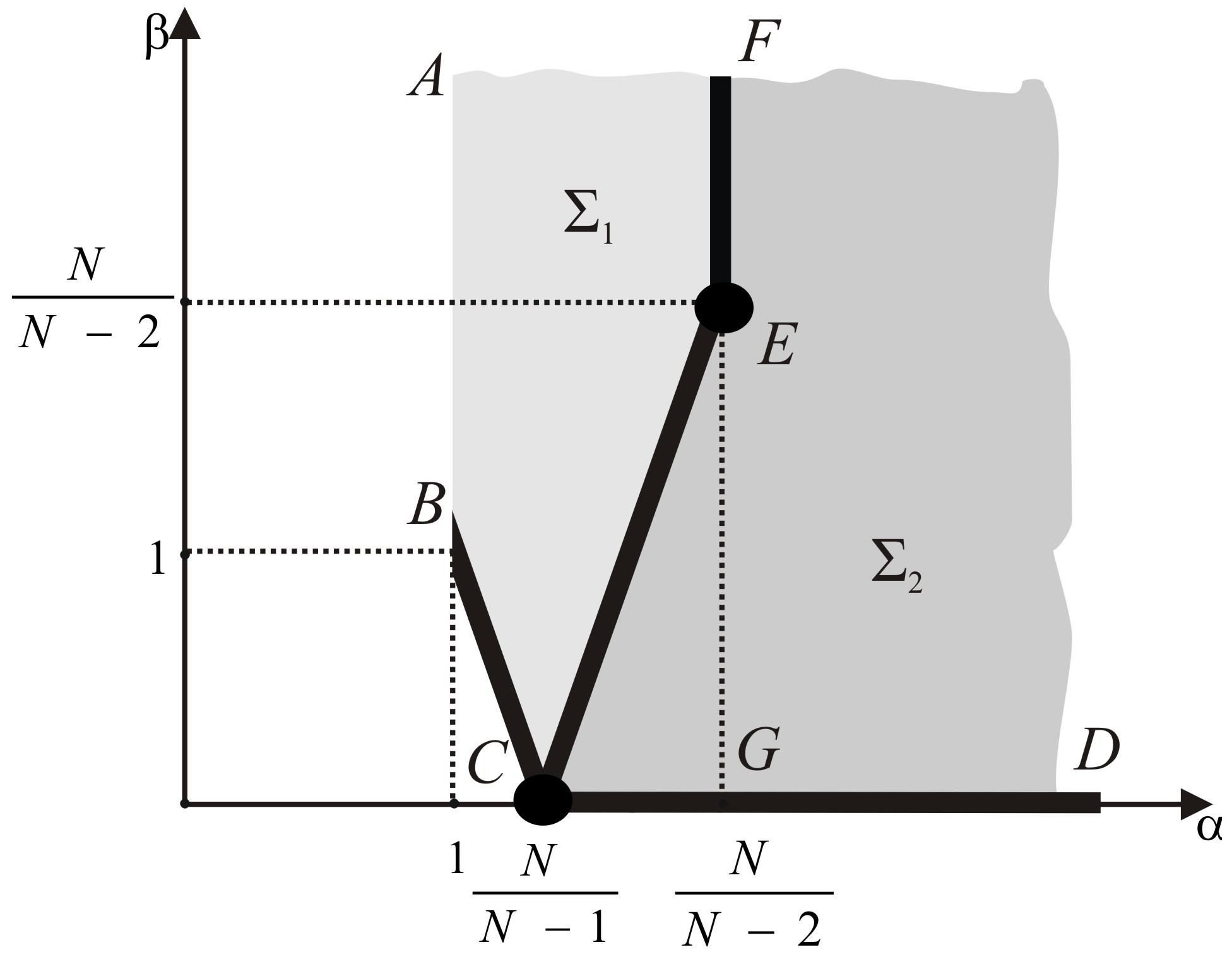
Figure 2: Plain $(\alpha,\beta)$

Since conditions (1) hold iff $\alpha>1$, $\alpha(N-1)+\beta-N\geq 0$ and $\beta\geq 0$ then we are restricted by the set involving the open unbounded domain whose boundary is the polyline $ABCD$, the open segment $(B,C)$ and the ray $[C,D)$. It is easy to see that Theorems 1.1-1.4 describe the behavior of $\sigma(-\Delta^{\varepsilon})$ for all $(\alpha,\beta)$ from this set. Indeed:

• In the point $C$ we have $q=\mathbf{q},\ p=\mathbf{d}^{N-1}\mathbf{q}$. This case is described by Theorem 1.1.

• On the open ray $(C,D)$ we have $q=\mathbf{q},\ p=0$. This case is described by Theorem 1.2.

• In the open domain $\Sigma_{1}$ whose boundary is the polyline $ABCEF$ we have $q=0$, $r=\infty$, $\mathrm{D}=\infty$. This case is described by Theorem 1.3. Here $p=0$ and therefore the homogenized operator is $-\Delta$.

• On the open segment $(B,C)$ we have $q=0,\ r=\infty,\ \mathrm{D}=\infty$. This case is also described by Theorem 1.3 but here $p=\mathbf{d}^{N-1}\mathbf{q}>0$ and the homogenized operator is $-\left(1+{1\over 2}\mathbf{d}^{N-1}\mathbf{q}\omega\right)^{-1}\Delta$.

• In the open segment $(C,E)$ we have either $q=0,\ r=\mathbf{d}^{N-1}\mathbf{q}^{-1},\ \mathrm{D}=\infty$, on the ray $[E,F)$ we have $q=0,\ \mathrm{D}=\mathbf{d}^{N-2},\ \mathrm{Q}<\infty$. These two cases are described by Theorem 1.4 (by the way in the point $E$ we have $\mathrm{Q}=\mathbf{d}^{-1}\mathbf{q}$, on the open ray $(E,F)$ we have $\mathrm{Q}=0$). In this case $\mathrm{V}>0$.

• On the open domain $\Sigma_{2}$ whose boundary is the polyline $FECD$ we have $r=0,\ \mathrm{D}=\infty$ (within the triangle $CEG$) or $\mathrm{D}=0$ (in the open domain whose boundary is the polyline $FGD$) or $\mathrm{D}=\mathbf{d}^{N-2},\ \mathrm{Q}=\infty$ (on the open segment $(E,G)$). This case is described by Theorem 1.4 but here $\mathrm{V}=0$, the homogenized operator is $-\left(\begin{matrix}\Delta&0\\ 0&\Delta\end{matrix}\right)$.

We remark that the spectrums of homogenized operators in $\Sigma_{1}$ and $\Sigma_{2}$ coincide but the multiplicity of each eigenvalue in $\Sigma_{2}$ is of two times grater then its multiplicity in $\Sigma_{1}$. This difference will be taken into account in Section 4 where a number-by-number convergence of the eigenvalues is studied.

Also we remark that in the case $N=2$ we have $\mathrm{D}=\infty$ for any $\alpha$. Therefore in this case in order to cover all types of homogenized problems we also have to consider the radius $d^{\varepsilon}$ that tends to zero faster then ${\varepsilon}^{\alpha}$, $\forall\alpha$. For example if $d^{\varepsilon}=\exp(-a/{\varepsilon}^{2})$ ($a\in(0,\infty)$) then $\mathrm{D}=a^{-1}$.

2 Auxiliary results

In this section we obtain some technical lemmas which are used in the proof of Theorems 1.1-1.4.

Let us introduce the list of notations. Recall that if the point $\tilde{x}$ belongs to $\Omega_{k}^{\varepsilon}$ ($k=1,2$) we assign to $\tilde{x}$ a pair $(x,k)$, where $x$ is a corresponding point in $\Omega^{\varepsilon}$; if the point $\tilde{x}$ belongs to $G_{i}^{\varepsilon}$ ($i\in\mathcal{I}({\varepsilon})$) we assign to $\tilde{x}$ a pair $(\varphi,z)$, where $\varphi=(\varphi_{1},{\dots},\varphi_{N-1})$ are the angular coordinates, $z\in[0,q^{\varepsilon}]$.

• $\square_{i}^{\varepsilon}$ be the cube in $\mathbb{R}^{N}$ with the center at $x_{i}^{\varepsilon}$, side-length ${\varepsilon}$ and edges which are parallel to the coordinate axes;

• $B_{ki}^{\varepsilon}=\left\{\tilde{x}=(x,k)\in\Omega_{k}^{\varepsilon}:\ d^{\varepsilon}\leq|x-x_{i}^{\varepsilon}|\leq{\varepsilon}/2\right\}$;

• $C_{ki}^{\varepsilon}=\left\{\tilde{x}=(x,k)\in\Omega_{k}^{\varepsilon}:\ |x-x_{i}^{\varepsilon}|={\varepsilon}/2\right\}$;

• $S_{i}^{\varepsilon}[\tau]=\left\{\tilde{x}=(\varphi,z)\in G_{i}^{\varepsilon}:\ z=\tau\right\},\ \tau\in[0,q^{\varepsilon}]$ (that is $S_{1i}^{\varepsilon}=S_{i}^{\varepsilon}[0],\ S_{2i}^{\varepsilon}=S_{i}^{\varepsilon}[q^{\varepsilon}]$);

• $\langle u\rangle_{B}$ (where either $B\subset M^{\varepsilon}$ or $B\subset\Omega$) be the mean value of the function $u\in L_{2}(B)$. That is $\displaystyle\langle u\rangle_{B}={1\over|B|}\int\limits_{B}ud\tilde{x}$, where $|B|$ is the volume of $B$;

• $\mathrm{S}_{N-1}$ be the $(N-1)$-dimensional unit sphere, $d\varphi=\left(\prod\limits_{k=1}^{N-1}\sin^{k-1}\varphi_{k}\right)d\varphi_{1}{\dots}d\varphi_{N-1}$ be the volume measure on $\mathrm{S}_{N-1}$;

• $C,\ C_{1},\ C_{2},$ etc. be generic positive constants independent of ${\varepsilon}$.

We introduce the operators $\widehat{X}^{\varepsilon}:C^{1}(\Omega)\to L_{2}(\Omega)$, $\widehat{\square}^{\varepsilon}:L_{2}(\Omega)\to L_{2}(\Omega)$, $\widehat{B}_{k}^{\varepsilon}:L_{2}(M^{\varepsilon})\to L_{2}(\Omega)$, $\widehat{S}_{k}^{\varepsilon}:L_{2}(M^{\varepsilon})\to L_{2}(\Omega)$ by the following formulae

$$\begin{matrix}[{\widehat{X}}^{\varepsilon}u](x)=\begin{cases}u(x_{i}^{\varepsilon}),&x\in\square_{i}^{\varepsilon}\\ 0,&\Omega\setminus\bigcup\limits_{i\in\mathcal{I}({\varepsilon})}\square_{i}^{\varepsilon};\end{cases}&[{\widehat{\square}}^{\varepsilon}u](x)=\begin{cases}\langle u\rangle_{\square_{i}^{\varepsilon}},&x\in\square_{i}^{\varepsilon}\\ 0,&\Omega\setminus\bigcup\limits_{i\in\mathcal{I}({\varepsilon})}\square_{i}^{\varepsilon};\end{cases}\\ \ \\ [\widehat{B}_{k}^{\varepsilon}u^{\varepsilon}](x)=\begin{cases}\langle u^{\varepsilon}\rangle_{B_{ki}^{\varepsilon}},&x\in\square_{i}^{\varepsilon}\\ 0,&\Omega\setminus\bigcup\limits_{i\in\mathcal{I}({\varepsilon})}\square_{i}^{\varepsilon};\end{cases}&[\widehat{S}_{k}^{\varepsilon}u^{\varepsilon}](x)=\begin{cases}\langle u^{\varepsilon}\rangle_{S_{ki}^{\varepsilon}},&x\in\square_{i}^{\varepsilon}\\ 0,&\Omega\setminus\bigcup\limits_{i\in\mathcal{I}({\varepsilon})}\square_{i}^{\varepsilon}.\end{cases}\end{matrix}$$ (9)

Also we introduce an extension operators $\Pi_{k}^{\varepsilon}:H^{1}(M^{\varepsilon})\to H^{1}(\Omega)$ ($k=1,2$) such that

$$\text{if }x\in\Omega^{\varepsilon}\text{ then }[\Pi_{k}^{\varepsilon}u^{\varepsilon}](x)=u^{\varepsilon}(\tilde{x}),\ \tilde{x}=(x,k)\in\Omega_{k}^{\varepsilon};$$

$$\forall u^{\varepsilon}\in H^{1}(\Omega_{k}^{\varepsilon}):\ \|\Pi_{k}^{\varepsilon}u^{\varepsilon}\|_{H^{1}(\Omega)}\leq C\|u^{\varepsilon}\|_{H^{1}(\Omega_{k}^{\varepsilon})}.$$

It is well-known (see e.g. [1, 12]) that such operators exist.

Lemma 2.1.

Let $u^{\varepsilon}\in H^{1}(M^{\varepsilon})$. Then the following inequalities hold:

$$\text{{\bf\rm I}.\qquad}\left|\langle u^{\varepsilon}\rangle_{S_{ki}^{\varepsilon}}-\langle u^{\varepsilon}\rangle_{B_{ki}^{\varepsilon}}\right|^{2}\leq C{\|\nabla u^{\varepsilon}\|^{2}_{L_{2}(B_{ki}^{\varepsilon})}\over\mathrm{D}^{\varepsilon}},\quad k=1,2,\ i\in\mathcal{I}({\varepsilon}),$$ (10)

$$\text{{\bf\rm II}.\qquad}\left|\langle\Pi_{k}^{\varepsilon}u^{\varepsilon}\rangle_{\square_{i}^{\varepsilon}}-\langle u^{\varepsilon}\rangle_{B_{ki}^{\varepsilon}}\right|^{2}\leq C{\varepsilon}^{2-N}\|\nabla\Pi_{k}^{\varepsilon}u^{\varepsilon}\|^{2}_{L_{2}(\square_{i}^{\varepsilon})},\quad k=1,2,\ i\in\mathcal{I}({\varepsilon}),$$ (11)

$$\text{{\bf\rm III}.\qquad}\left|\langle u^{\varepsilon}\rangle_{S_{i}^{\varepsilon}[\tau_{1}]}-\langle u^{\varepsilon}\rangle_{S_{i}^{\varepsilon}[\tau_{2}]}\right|^{2}\leq\omega^{-1}\|\nabla^{\varepsilon}u^{\varepsilon}\|^{2}_{L_{2}(G_{i}^{\varepsilon})}{q^{\varepsilon}\over(d^{\varepsilon})^{N-1}},\quad\forall\tau_{1},\tau_{2}\in[0,q^{\varepsilon}],\ i\in\mathcal{I}({\varepsilon}).$$ (12)

Proof. I. Let us fix $k$ and $i$, and let us introduce a spherical coordinates $(\varphi,r)$ in $B_{ki}^{\varepsilon}$. Here $r$ is a distance to $x_{i}^{\varepsilon}$ ($r\geq d^{\varepsilon}$), $\varphi=(\varphi_{1},{\dots},\varphi_{N-1})$ are the angular coordinates. Let $x=(\varphi,d^{\varepsilon})\in S_{ki}^{\varepsilon}$, $y=(\varphi,r)\in B_{ki}^{\varepsilon}$. We have

$$u^{\varepsilon}(x)-u^{\varepsilon}(y)=-\int\limits_{d^{\varepsilon}}^{r}{\partial u^{\varepsilon}(\varphi,\tau)\over\partial\tau}d\tau.$$

Then we multiply this equality by $r^{N-1}d\varphi dr$, integrate from $d^{\varepsilon}$ to ${\varepsilon}/2$ (with respect to $r$) and over $\mathrm{S}_{N-1}$ (with respect to $\varphi$), divide by $|B_{ki}^{\varepsilon}|$ and square. Using Cauchy inequality we obtain:

$$\left|\langle u^{\varepsilon}\rangle_{S_{ki}^{\varepsilon}}-\langle u^{\varepsilon}\rangle_{B_{ki}^{\varepsilon}}\right|^{2}={1\over|B_{i}^{\varepsilon}|^{2}}\left|\int\limits_{d^{\varepsilon}}^{{\varepsilon}/2}r^{N-1}\int\limits_{\mathrm{S}_{N-1}}\int\limits_{d^{\varepsilon}}^{r}{\partial u^{\varepsilon}(\varphi,\tau)\over\partial\tau}(\varphi,\tau)d\tau d\varphi dr\right|^{2}\leq$$

$$\leq{\omega\over|B_{i}^{\varepsilon}|^{2}}\left(\displaystyle{{\varepsilon}\over 2}-d^{\varepsilon}\right)\displaystyle\int\limits_{d^{\varepsilon}}^{{\varepsilon}/2}r^{2(N-1)}dr\int\limits_{\mathrm{S}_{N-1}}\int\limits_{d^{\varepsilon}}^{{\varepsilon}/2}\left|{\partial u^{\varepsilon}(\varphi,\tau)\over\partial\tau}\right|^{2}\tau^{N-1}d\tau d\varphi\int\limits_{d^{\varepsilon}}^{{\varepsilon}/2}{d\tau\over\tau^{N-1}}\leq C{\|\nabla u^{\varepsilon}\|^{2}_{L_{2}(B_{ki}^{\varepsilon})}\over\mathrm{D}^{\varepsilon}}.$$

II. The inequality (11) is a particular case of Lemma 2.1 from [18].

III. Let $\tilde{x}=(\varphi,\tau_{1})\in S_{i}^{\varepsilon}[\tau_{1}]$, $\tilde{y}=(\varphi,\tau_{2})\in S_{i}^{\varepsilon}[\tau_{2}]$. Then $\displaystyle u^{\varepsilon}(\tilde{x})-u^{\varepsilon}(\tilde{y})=-\int\limits_{\tau_{1}}^{\tau_{2}}\displaystyle{\partial u^{\varepsilon}(\varphi,\tau)\over\partial\tau}d\tau,$ and we obtain

$$\left|\langle u^{\varepsilon}\rangle_{S_{i}^{\varepsilon}[\tau_{1}]}-\langle u^{\varepsilon}\rangle_{S_{i}^{\varepsilon}[\tau_{2}]}\right|^{2}\leq\\ \leq\omega^{-1}|\tau_{1}-\tau_{2}|\int\limits_{\mathrm{S}_{N-1}}\int\limits_{\tau_{1}}^{\tau_{2}}\left({\partial u^{\varepsilon}(\varphi,\tau)\over\partial\tau}\right)^{2}d\tau d\varphi_{1}{\dots}d\varphi_{N-1}\leq\omega^{-1}\|\nabla u^{\varepsilon}\|^{2}_{L_{2}(G_{i}^{\varepsilon})}{q^{\varepsilon}\over(d^{\varepsilon})^{N-1}}.\quad\square$$

Corollary 2.2.

Let $u^{\varepsilon}\in H^{1}(M^{\varepsilon})$, $\|\nabla^{\varepsilon}u^{\varepsilon}\|^{2}_{L_{2}(M^{\varepsilon})}<C$ and $\Pi_{k}^{\varepsilon}u^{\varepsilon}\underset{{\varepsilon}\to 0}{\to}u_{k}$ strongly in $L_{2}(\Omega)$ ($k=1,2$). Then we have

$$\text{if\ }\mathrm{D}=\infty:\quad \widehat{S}_{k}^{\varepsilon}u^{\varepsilon}\underset{{\varepsilon}\to 0}{\to}u_{k},$$ (13)

$$\widehat{B}_{k}^{\varepsilon}u^{\varepsilon}\underset{{\varepsilon}\to 0}{\to}u_{k},$$ (14)

$$\text{\ if\ }\displaystyle\lim\limits_{{\varepsilon}\to 0}{(d^{\varepsilon})^{N-1}\over{\varepsilon}^{N}}=0:\quad \displaystyle{(d^{\varepsilon})^{N-1}\over{\varepsilon}^{N}}\|\widehat{S}_{k}^{\varepsilon}u^{\varepsilon}\|^{2}_{L_{2}(\Omega)}\underset{{\varepsilon}\to 0}{\to}0,$$ (15)

$$\text{if\ }r=\mathrm{D}=\infty:\quad u_{1}=u_{2}\text{\ \ {\rm and}\ }\lim\limits_{{\varepsilon}\to 0}\displaystyle\sum\limits_{i\in\mathcal{I}({\varepsilon})}\|u^{\varepsilon}\|^{2}_{L_{2}(G_{i}^{\varepsilon})}=p\omega\|u_{1}\|^{2}_{L_{2}(\Omega)}.$$ (16)

Proof. We present the proof only for the statement (13) (another statements are proved similarly using Lemma 2.1). One has:

$$\|\widehat{S}_{k}^{\varepsilon}u^{\varepsilon}-u_{k}^{\varepsilon}\|_{L_{2}(\Omega)}\leq\left(\|\widehat{S}_{k}^{\varepsilon}u^{\varepsilon}-\widehat{B}_{k}^{\varepsilon}u^{\varepsilon}\|_{L_{2}(\Omega)}+\|\widehat{B}_{k}^{\varepsilon}u^{\varepsilon}-\widehat{\square}^{\varepsilon}\Pi_{k}^{\varepsilon}u^{\varepsilon}\|_{L_{2}(\Omega)}+\right.\\ \left.+\|\widehat{\square}^{\varepsilon}\Pi_{k}^{\varepsilon}u^{\varepsilon}-\Pi_{k}^{\varepsilon}u^{\varepsilon}\|_{L_{2}(\Omega)}+\|\Pi_{k}^{\varepsilon}u^{\varepsilon}-u_{k}\|_{L_{2}(\Omega)}\right).$$ (17)

Due to the inequality (10) the first term in (17) tends to zero if $\mathrm{D}=\infty$:

$$\|\widehat{S}_{k}^{\varepsilon}u^{\varepsilon}-\widehat{B}_{k}^{\varepsilon}u^{\varepsilon}\|^{2}_{L_{2}(\Omega)}={\varepsilon}^{N}\sum\limits_{i\in\mathcal{I}({\varepsilon})}\left|\langle u^{\varepsilon}\rangle_{S_{ki}^{\varepsilon}}-\langle u^{\varepsilon}\rangle_{B_{ki}^{\varepsilon}}\right|^{2}\leq C{{\varepsilon}^{N}\over\mathrm{D}^{\varepsilon}}\|\nabla^{\varepsilon}u^{\varepsilon}\|^{2}_{L_{2}(\Omega_{k}^{\varepsilon})}\underset{{\varepsilon}\to 0}{\to}0.$$

In a similar way inequality (11) implies that the second term also tends to zero. The third term tends to zero by virtue of the Poincare inequality for the cube $\square_{i}^{\varepsilon}$. And finally the last term tends to zero by the given data. Thus the statement (13) is proved. $\square$

Lemma 2.3.

Let $q=p=0$. Let $u^{\varepsilon}\in H^{1}(M^{\varepsilon})$, $\|\nabla^{\varepsilon}u^{\varepsilon}\|^{2}_{L_{2}(M^{\varepsilon})}<C$. Then

$$\lim\limits_{{\varepsilon}\to 0}\sum\limits_{i\in\mathcal{I}({\varepsilon})}\|u^{\varepsilon}\|^{2}_{L_{2}(G_{i}^{\varepsilon})}=0.$$

Proof follows directly from the following inequality: for $\forall u^{\varepsilon}\in H^{1}(M^{\varepsilon})$

$$\|u^{\varepsilon}\|^{2}_{G_{i}^{\varepsilon}}\leq C\left\{(q^{\varepsilon})^{2}\|\nabla u^{\varepsilon}\|^{2}_{L_{2}(G_{i}^{\varepsilon})}+{{q^{\varepsilon}}(d^{\varepsilon})^{N-1}\over{\varepsilon}^{N}}\|u^{\varepsilon}\|^{2}_{L_{2}(B_{i}^{\varepsilon})}+{q^{\varepsilon}(d^{\varepsilon})^{N-1}\over\mathrm{D}^{\varepsilon}}\|\nabla u^{\varepsilon}\|^{2}_{L_{2}(B_{i}^{\varepsilon})}\right\}.$$ (18)

This inequality is proved in [17] (Lemma 2.2) for $N=2$. For $N>2$ the proof is fully similar. $\square$

Lemma 2.4.

Let $q>0$. Let $\lambda^{\varepsilon}\in\sigma(-\Delta^{\varepsilon})$, $u^{\varepsilon}$ be the corresponding eigenfunction such that $\|u^{\varepsilon}\|_{L_{2}(M^{\varepsilon})}=1$. Suppose that $\lambda^{\varepsilon}\underset{{\varepsilon}\to 0}{\to}\lambda_{0}\notin\bigcup\limits_{n\in\mathbb{N}}\left\{(\pi n)^{2}q^{-2}\right\}$ and $\Pi^{\varepsilon}_{k}u^{\varepsilon}\underset{{\varepsilon}\to 0}{\to}u_{k}\in H_{0}^{1}(\Omega)$ ($k=1,2$) strongly in $L_{2}(\Omega)$.

Then if $p>0$ one has

$$\lim\limits_{{\varepsilon}\to 0}\sum\limits_{i\in\mathcal{I}({\varepsilon})}\|u^{\varepsilon}\|^{2}_{L_{2}(G_{i}^{\varepsilon})}=p\omega\bigg{\{}k_{1}\left(\|u_{1}\|_{L_{2}(\Omega)}^{2}+\|u_{2}\|_{L_{2}(\Omega)}^{2}\right)+2k_{2}(u_{1},u_{2})_{L_{2}(\Omega)}\bigg{\}},$$ (19)

where $k_{1}=\displaystyle{q\sqrt{\lambda_{0}}-\sin(q\sqrt{\lambda_{0}})\cos(q\sqrt{\lambda_{0}})\over 2q\sqrt{\lambda_{0}}\sin^{2}(q\sqrt{\lambda_{0}})}$, $k_{2}=-\displaystyle{q\sqrt{\lambda_{0}}\cos(q\sqrt{\lambda_{0}})-\sin(q\sqrt{\lambda_{0}})\over 2q\sqrt{\lambda_{0}}\sin^{2}(q\sqrt{\lambda_{0}})}$.

If $p=0$ one has

$$\lim\limits_{{\varepsilon}\to 0}\sum\limits_{i\in\mathcal{I}({\varepsilon})}\|u^{\varepsilon}\|^{2}_{L_{2}(G_{i}^{\varepsilon})}=0.$$ (20)

Proof. We introduce on $G_{i}^{\varepsilon}$ the function $v_{i}^{\varepsilon}(\varphi,z)=\langle u^{\varepsilon}\rangle_{S_{i}^{\varepsilon}[z]}$ (it is clear that $v_{i}^{\varepsilon}$ is independent of $\varphi$). By the Poincare inequality

$$\sum\limits_{i\in\mathcal{I}({\varepsilon})}\|u^{\varepsilon}-v_{i}^{\varepsilon}\|^{2}_{G_{i}^{\varepsilon}}\leq C(d^{\varepsilon})^{2}\sum\limits_{i\in\mathcal{I}({\varepsilon})}\|\nabla^{\varepsilon}u^{\varepsilon}\|^{2}_{L_{2}(G_{i}^{\varepsilon})}\leq C(d^{\varepsilon})^{2}\lambda^{\varepsilon}.$$ (21)

Since $-\Delta^{\varepsilon}u^{\varepsilon}=\lambda^{\varepsilon}u^{\varepsilon}$ then it is easy to see that

$$-(v_{i}^{\varepsilon})^{\prime\prime}=\lambda^{\varepsilon}v_{i}^{\varepsilon},\ z\in(0,q^{\varepsilon}),\quad v_{i}^{\varepsilon}(0)=\langle u^{\varepsilon}\rangle_{S_{1i}^{\varepsilon}},\quad v_{i}^{\varepsilon}(q^{\varepsilon})=\langle u^{\varepsilon}\rangle_{S_{2i}^{\varepsilon}}.$$ (22)

So long as $\lambda^{\varepsilon}\underset{{\varepsilon}\to 0}{\to}\lambda_{0}\notin\bigcup\limits_{n\in\mathbb{N}}\left\{(\pi n)^{2}q^{-2}\right\}$ and $q^{\varepsilon}\underset{{\varepsilon}\to 0}{\to}q$ then for sufficiently small ${\varepsilon}$ $\lambda^{\varepsilon}\not\in\bigcup\limits_{n\in\mathbb{N}}\left\{{(\pi n)^{2}(q^{\varepsilon})^{-2}}\right\}$. Therefore the problem (22) has the unique solution

$$v_{i}^{\varepsilon}(z)=A_{i}^{\varepsilon}\sin(z\sqrt{\lambda^{\varepsilon}})+B_{i}^{\varepsilon}\cos(z\sqrt{\lambda^{\varepsilon}}),\text{ where }A_{i}^{\varepsilon}={\langle u^{\varepsilon}\rangle_{S_{2i}^{\varepsilon}}-\langle u^{\varepsilon}\rangle_{S_{1i}^{\varepsilon}}\cos(q^{\varepsilon}\sqrt{\lambda^{\varepsilon}})\over\sin(q^{\varepsilon}\sqrt{\lambda^{\varepsilon}})},\ B_{i}^{\varepsilon}=\langle u^{\varepsilon}\rangle_{S_{1i}^{\varepsilon}}.$$

Direct computations show that

$$\|v_{i}^{\varepsilon}\|^{2}_{L_{2}(G_{i}^{\varepsilon})}=\omega(d^{\varepsilon})^{N-1}q^{\varepsilon}\bigg{\{}k^{\varepsilon}_{1}\left(\langle u^{\varepsilon}\rangle^{2}_{S_{1i}^{\varepsilon}}+\langle u^{\varepsilon}\rangle^{2}_{S_{2i}^{\varepsilon}}\right)+2k^{\varepsilon}_{2}\langle u^{\varepsilon}\rangle_{S_{1i}^{\varepsilon}}\cdot\langle u^{\varepsilon}\rangle_{S_{2i}^{\varepsilon}}\bigg{\}},$$

where $\displaystyle k_{1}^{\varepsilon}=\displaystyle{q\sqrt{\lambda^{\varepsilon}}-\sin(q^{\varepsilon}\sqrt{\lambda^{\varepsilon}})\cos(q^{\varepsilon}\sqrt{\lambda^{\varepsilon}})\over 2q^{\varepsilon}\sqrt{\lambda^{\varepsilon}}\sin^{2}(q^{\varepsilon}\sqrt{\lambda^{\varepsilon}})}$, $k_{2}=-\displaystyle{q\sqrt{\lambda^{\varepsilon}}\cos(q^{\varepsilon}\sqrt{\lambda^{\varepsilon}})-\sin(q^{\varepsilon}\sqrt{\lambda^{\varepsilon}})\over 2q^{\varepsilon}\sqrt{\lambda^{\varepsilon}}\sin^{2}(q^{\varepsilon}\sqrt{\lambda^{\varepsilon}})}$. Therefore

$$\sum\limits_{i\in\mathcal{I}({\varepsilon})}\|v_{i}^{\varepsilon}\|^{2}_{L_{2}(G_{i}^{\varepsilon})}=\\ =\omega{(d^{\varepsilon})^{N-1}q^{\varepsilon}\over{\varepsilon}^{N}}\bigg{\{}k^{\varepsilon}_{1}\left(\|\widehat{S}_{1}^{\varepsilon}u^{\varepsilon}\|^{2}_{L_{2}(\Omega)}+\|\widehat{S}_{2}^{\varepsilon}u^{\varepsilon}\|^{2}_{L_{2}(\Omega)}\right)+2k^{\varepsilon}_{2}(\widehat{S}_{1}^{\varepsilon}u^{\varepsilon},\widehat{S}_{2}^{\varepsilon}u^{\varepsilon})_{L_{2}(\Omega)}\bigg{\}}.$$ (23)

Then (19) follows directly from (23), (21) and Corollary 2.2 (see (13)). Similarly (20) follows from (23), (21) and (15). Lemma is proved.  $\square$

3 Proof of the main Theorems

3.1 Proof of Theorem 1.1

Step 1. Firstly we prove that condition (A) of the Hausdorff convergence holds. Let $\lambda^{\varepsilon}\in\sigma(-\Delta^{\varepsilon})$ and $\lambda^{\varepsilon}\underset{{\varepsilon}\to 0}{\to}\lambda_{0}$. If $\lambda_{0}\in\bigcup\limits_{n\in\mathbb{N}}\left\{{(\pi n)^{2}q^{-2}}\right\}$ then (A) is proved. Therefore we are interested in the case $\lambda_{0}\notin\bigcup\limits_{n\in\mathbb{N}}\left\{{(\pi n)^{2}q^{-2}}\right\}$.

Let $u^{\varepsilon}$ be the eigenfunction that correspond to $\lambda^{\varepsilon}$ and $\|u^{\varepsilon}\|_{L_{2}(M^{\varepsilon})}=1$ (and therefore $\|\nabla^{\varepsilon}u^{\varepsilon}\|^{2}_{L_{2}(M^{\varepsilon})}=\lambda^{\varepsilon}$). Since the functions $u^{\varepsilon}$ are bounded in $H_{0}^{1}(M^{\varepsilon})$ uniformly in ${\varepsilon}$ then $\Pi_{k}^{\varepsilon}u^{\varepsilon}$ ($k=1,2$) are also bounded in $H_{0}^{1}(M^{\varepsilon})$ uniformly in ${\varepsilon}$. Therefore due to the embedding theorem there exists a subsequence (still denoted by ${\varepsilon}$) such that

$$\Pi_{k}^{\varepsilon}u^{\varepsilon}\underset{{\varepsilon}\to 0}{\to}u_{k}\in H_{0}^{1}(\Omega)\quad(k=1,2)\quad\text{\ strongly in }L_{2}(\Omega)\text{\ and weakly in }H^{1}(\Omega).$$

By Lemma 2.4 we have

$$1=\lim\limits_{{\varepsilon}\to 0}\|u^{\varepsilon}\|^{2}_{L_{2}(M^{\varepsilon})}=\|u_{1}\|^{2}_{L_{2}(\Omega)}+\|u_{2}\|^{2}_{L_{2}(\Omega)}+p\omega\bigg{\{}k_{1}\left(\|u_{1}\|^{2}_{L_{2}(\Omega)}+\|u_{2}\|^{2}_{L_{2}(\Omega)}\right)+2k_{2}(u_{1},u_{2})_{L_{2}(\Omega)}\bigg{\}}$$

and therefore $\mathrm{U}=\left(\begin{matrix}u_{1}\\ u_{2}\end{matrix}\right)\not=0$. We prove that $\mathrm{A}(\lambda_{0})\mathrm{U}=0$.

For an arbitrary $w^{\varepsilon}\in H^{1}_{0}(M^{\varepsilon})$ we have:

$$\int\limits_{M^{\varepsilon}}\nabla^{\varepsilon}u^{\varepsilon}\cdot\nabla^{\varepsilon}w^{\varepsilon}d\tilde{x}-\lambda^{\varepsilon}\int\limits_{M^{\varepsilon}}u^{\varepsilon}w^{\varepsilon}d\tilde{x}=0.$$ (24)

Let us introduce the following test function $w^{\varepsilon}$:

$$w^{\varepsilon}(\tilde{x})=\begin{cases}w_{k}(x)+\displaystyle\sum\limits_{i\in\mathcal{I}({\varepsilon})}\bigg{(}w_{k}(x_{i}^{\varepsilon})-w_{k}(x)\bigg{)}\cdot\varphi\left({|x-x_{i}^{\varepsilon}|\over d^{\varepsilon}}\right),&\tilde{x}=(x,k)\in\Omega_{k}^{\varepsilon},\ k=1,2,\\ v_{i}^{\varepsilon}(z),&\tilde{x}=(\varphi,z)\in G_{i}^{\varepsilon},\ i\in\mathcal{I}({\varepsilon}).\end{cases}$$ (25)

Here $w_{k}(x)\in C_{0}^{\infty}(\Omega)$ ($k=1,2$) are arbitrary functions, $\varphi(r):[0,\infty)\to\mathbb{R}$ is a smooth positive function equal to $1$ as $r\leq 1$ and equal to $0$ as $r\geq 2$, $v_{i}^{\varepsilon}(z)$ is defined by the formula:

$$v_{i}^{\varepsilon}(z)=A_{i}^{\varepsilon}\sin(z\sqrt{\lambda^{\varepsilon}})+B_{i}^{\varepsilon}\cos(z\sqrt{\lambda^{\varepsilon}}),\text{ where }A_{i}^{\varepsilon}={w_{2}(x_{i}^{\varepsilon})-w_{1}(x_{i}^{\varepsilon})\cos(q^{\varepsilon}\sqrt{\lambda^{\varepsilon}})\over\sin(q^{\varepsilon}\sqrt{\lambda^{\varepsilon}})},\ B_{i}^{\varepsilon}=w_{1}(x_{i}^{\varepsilon})$$

(we suppose that ${\varepsilon}$ is sufficiently small so that $\lambda^{\varepsilon}\not\in\bigcup\limits_{n\in\mathbb{N}}\left\{{(\pi n)^{2}(q^{\varepsilon})^{-2}}\right\}$). It is easy to see that

$$-(v_{i}^{\varepsilon})^{\prime\prime}=\lambda^{\varepsilon}v_{i}^{\varepsilon},\ z\in(0,q^{\varepsilon}),\quad v_{i}^{\varepsilon}(0)=w_{1}(x_{i}^{\varepsilon}),\quad v_{i}^{\varepsilon}(q^{\varepsilon})=w_{2}(x_{i}^{\varepsilon}).$$

We denote $\varphi_{i}^{\varepsilon}=\varphi\left({|x-x_{i}^{\varepsilon}|/d^{\varepsilon}}\right)$.

Substituting this $w^{\varepsilon}$ into (24) and taking into account that

$$\int\limits_{G_{i}^{\varepsilon}}\bigg{(}\nabla^{\varepsilon}u^{\varepsilon}\cdot\nabla^{\varepsilon}w^{\varepsilon}-\lambda^{\varepsilon}u^{\varepsilon}w^{\varepsilon}\bigg{)}d\tilde{x}=(d^{\varepsilon})^{N-1}\omega\left(-\langle u^{\varepsilon}\rangle_{S_{1i}^{\varepsilon}}{\partial v_{i}^{\varepsilon}(0)\over\partial z}+\langle u^{\varepsilon}\rangle_{S_{2i}^{\varepsilon}}{\partial v_{i}^{\varepsilon}(q^{\varepsilon})\over\partial z}\right),$$

we obtain

$$0=\sum\limits_{k=1,2}\int\limits_{\Omega^{\varepsilon}}\bigg{(}\nabla(\Pi_{k}^{\varepsilon}u^{\varepsilon})\cdot\nabla w_{k}-\lambda^{\varepsilon}(\Pi_{k}^{\varepsilon}u^{\varepsilon})w_{k}\bigg{)}dx+\\ +\sum\limits_{i\in\mathcal{I}({\varepsilon})}{(d^{\varepsilon})^{N-1}\omega\sqrt{\lambda^{\varepsilon}}\over\sin(q^{\varepsilon}\sqrt{\lambda^{\varepsilon}})}\bigg{(}\langle u^{\varepsilon}\rangle_{S_{1i}^{\varepsilon}}\cdot\cos(q^{\varepsilon}\sqrt{\lambda^{\varepsilon}})-\langle u^{\varepsilon}\rangle_{S_{2i}^{\varepsilon}}\bigg{)}\cdot w_{1}(x_{i}^{\varepsilon})+\\ +\sum\limits_{i\in\mathcal{I}({\varepsilon})}{(d^{\varepsilon})^{N-1}\omega\sqrt{\lambda^{\varepsilon}}\over\sin(q^{\varepsilon}\sqrt{\lambda^{\varepsilon}})}\bigg{(}\langle u^{\varepsilon}\rangle_{S_{2i}^{\varepsilon}}\cdot\cos(q^{\varepsilon}\sqrt{\lambda^{\varepsilon}})-\langle u^{\varepsilon}\rangle_{S_{1i}^{\varepsilon}}\bigg{)}\cdot w_{2}(x_{i}^{\varepsilon})+\delta^{\varepsilon}$$ (26)

and the remainder

$$\delta^{\varepsilon}=\sum\limits_{k=1,2}\int\limits_{\Omega_{k}^{\varepsilon}}\displaystyle\sum\limits_{i\in\mathcal{I}({\varepsilon})}\bigg{[}\nabla\bigg{(}\big{(}w_{k}(x_{i}^{\varepsilon})-w_{k}(x)\big{)}\varphi_{i}^{\varepsilon}(x)\bigg{)}\cdot\nabla u^{\varepsilon}(x)-\\ -\lambda^{\varepsilon}\big{(}w_{k}(x_{i}^{\varepsilon})-w_{k}(x)\big{)}\varphi_{i}^{\varepsilon}(x)u^{\varepsilon}(x)\bigg{]}dx$$ (27)

is vanishingly small as ${\varepsilon}\to 0$ (since $|w(x_{i}^{\varepsilon})-w^{\varepsilon}(x)|<Cd^{\varepsilon}$ for $x\in\mathrm{supp}(\varphi_{i}^{\varepsilon})$ ):

$$|\delta^{\varepsilon}|\leq C\|u^{\varepsilon}\|^{2}_{H^{1}(\Omega)}\sum\limits_{i\in\mathcal{I}({\varepsilon})}\left|\mathrm{supp}(\varphi_{i}^{\varepsilon})\right|\underset{{\varepsilon}\to 0}{\to}0.$$

We rewrite (26) in the form

$$0=\sum\limits_{k=1,2}\int\limits_{\Omega^{\varepsilon}}\bigg{(}\nabla(\Pi_{k}^{\varepsilon}u^{\varepsilon})\cdot\nabla w_{k}-\lambda^{\varepsilon}(\Pi_{k}^{\varepsilon}u^{\varepsilon})w_{k}\bigg{)}dx+\\ +{(d^{\varepsilon})^{N-1}\omega\over{\varepsilon}^{N}}\cdot{\sqrt{\lambda^{\varepsilon}}\over\sin(q^{\varepsilon}\sqrt{\lambda^{\varepsilon}})}\int\limits_{\Omega}\bigg{(}\widehat{S}_{1}^{\varepsilon}u^{\varepsilon}\cdot\cos(q^{\varepsilon}\sqrt{\lambda^{\varepsilon}})-\widehat{S}_{2}^{\varepsilon}u^{\varepsilon}\bigg{)}\widehat{X}^{\varepsilon}w_{1}dx+\\ +{(d^{\varepsilon})^{N-1}\omega\over{\varepsilon}^{N}}\cdot{\sqrt{\lambda^{\varepsilon}}\over\sin(q^{\varepsilon}\sqrt{\lambda^{\varepsilon}})}\int\limits_{\Omega}\bigg{(}\widehat{S}_{2}^{\varepsilon}u^{\varepsilon}\cdot\cos(q^{\varepsilon}\sqrt{\lambda^{\varepsilon}})-\widehat{S}_{1}^{\varepsilon}u^{\varepsilon}\bigg{)}\widehat{X}^{\varepsilon}w_{2}dx+\delta^{\varepsilon},$$ (28)

where the operators $\widehat{X}^{\varepsilon},\ \widehat{S}_{k}^{\varepsilon}\ (k=1,2)$ are defined by the formulae (9).

It is obvious that for any $w\in C^{1}(\Omega)$ $\widehat{X}^{\varepsilon}w\underset{{\varepsilon}\to 0}{\to}w$ strongly in $L_{2}(\Omega)$. Moreover since $p,q>0$ then $\mathrm{D}=\infty$ and therefore due to Corollary 2.2 (see (13)) $\widehat{S}_{k}^{\varepsilon}u^{\varepsilon}\underset{{\varepsilon}\to 0}{\to}u_{k}$ strongly in $L_{2}(\Omega)$. Therefore passing to the limit (as ${\varepsilon}\to\ 0$) in (28) we conclude that

$$0=\sum\limits_{k=1,2}\int\limits_{\Omega}\bigg{(}\nabla u_{k}\cdot\nabla w_{k}-\lambda_{0}u_{k}w_{k}\bigg{)}dx+{p\omega\over q}{\sqrt{\lambda_{0}}\over\sin(q\sqrt{\lambda_{0}})}\int\limits_{\Omega}\bigg{(}u_{1}\cdot\cos(q\sqrt{\lambda_{0}})-u_{2}\bigg{)}w_{1}dx+\\ +{p\omega\over q}{\sqrt{\lambda_{0}}\over\sin(q\sqrt{\lambda_{0}})}\int\limits_{\Omega}\bigg{(}u_{2}\cdot\cos(q\sqrt{\lambda_{0}})-u_{1}\bigg{)}w_{2}dx,\quad\forall w_{1},w_{2}\in C_{0}^{\infty}(\Omega).$$ (29)

It is easy to see that (29) implies that $\mathrm{A}(\lambda_{0})\mathrm{U}=0$. The fulfilment (A) is proved.

Step 2. Let us prove the fulfilment of the condition (B) of the Hausdorff convergence.

Firstly suppose that $\lambda_{0}\in\sigma(\mathrm{A}(\lambda))$. We have to prove that there exists $\lambda^{\varepsilon}\in\sigma(-\Delta^{\varepsilon})$ such that $\lambda^{\varepsilon}\underset{{\varepsilon}\to 0}{\to}\lambda_{0}$.

Proving this indirectly we assume the opposite. Then the subsequence (still denoted by ${\varepsilon}$) and a positive number $\delta$ exist such that

$$\min\limits_{\lambda^{\varepsilon}\in\sigma(-\Delta^{\varepsilon})}|\lambda_{0}-\lambda^{\varepsilon}|>\delta.$$ (30)

Since $\lambda_{0}$ belongs to the spectrum of $\mathrm{A}(\lambda)$ there exists $\mathrm{F}=\left(\begin{matrix}f_{1}\\ f_{2}\end{matrix}\right)\in[L_{2}(\Omega)]^{2}$ such that

$$\mathrm{F}\not\in\mathrm{Im}\mathrm{A}(\lambda_{0}).$$ (31)

Let us consider the following problem on $M^{\varepsilon}$:

$$-\Delta^{\varepsilon}u-\lambda_{0}u=f^{\varepsilon}.$$ (32)

In view of (30) this problem has the unique solution $u^{\varepsilon}(\tilde{x})\in H_{0}^{1}(M^{\varepsilon})$ for an arbitrary $f^{\varepsilon}\in L_{2}(M^{\varepsilon})$. We set

$$f^{\varepsilon}(\tilde{x})=\begin{cases}f_{k}(x),&\tilde{x}\in(x,k),\ k=1,2,\\ 0,&\tilde{x}\in G_{i}^{\varepsilon},\ i\in\mathcal{I}({\varepsilon}).\end{cases}$$

One has

$$\|u^{\varepsilon}\|_{L_{2}(M^{\varepsilon})}\leq{\|f^{\varepsilon}\|_{L_{2}(M^{\varepsilon})}\over\delta}\leq C_{1},$$

$$\|\nabla^{\varepsilon}u^{\varepsilon}\|^{2}_{L_{2}(M^{\varepsilon})}\leq|\lambda_{0}|\cdot\|u^{\varepsilon}\|_{L_{2}(M^{\varepsilon})}^{2}+\left|(f^{\varepsilon},u^{\varepsilon})_{L_{2}(M^{\varepsilon})}\right|\leq C_{2}.$$

Therefore $\|\Pi_{k}^{\varepsilon}u^{\varepsilon}\|_{H_{1}(\Omega)}\leq C$ ($k=1,2$) and by the embedding theorem there exists a subsequence (still denoted by ${\varepsilon}$) such that $\Pi_{k}^{\varepsilon}u^{\varepsilon}\underset{{\varepsilon}\to 0}{\to}u_{k}\in H_{0}^{1}(\Omega)\quad(k=1,2)$.

For an arbitrary $w^{\varepsilon}\in H^{1}_{0}(M^{\varepsilon})$ we have the following equality:

$$\int\limits_{M^{\varepsilon}}\left(\nabla^{\varepsilon}u^{\varepsilon}\cdot\nabla^{\varepsilon}w^{\varepsilon}-\lambda^{\varepsilon}u^{\varepsilon}w^{\varepsilon}-f^{\varepsilon}w^{\varepsilon}\right)d\tilde{x}=0.$$ (33)

Let us substitute into (33) the function $w^{\varepsilon}$ defined by the formula (25) and pass to the limit in (33) as ${\varepsilon}\to 0$. Similarly to ”Step 1” we prove that

$$\mathrm{A}(\lambda_{0})\mathrm{U}=\mathrm{F},\quad\mathrm{U}=\left(\begin{matrix}u_{1}\\ u_{2}\end{matrix}\right).$$

Thus we obtain a contradiction to (31).

In order to complite the verification of the fulfilment of (B) we have to prove that for any $\lambda_{0}\in\bigcup\limits_{n\in\mathbb{N}}\left\{{(\pi n)^{2}q^{-2}}\right\}$ there exists $\lambda^{\varepsilon}\in\sigma(-\Delta^{\varepsilon})$ such that $\lambda^{\varepsilon}\underset{{\varepsilon}\to 0}{\to}\lambda_{0}$. But this fact follows directly from the structure of $\sigma(\mathrm{A}(\lambda_{0}))$ (see (2)). Indeed (2) implies that for some $n\in\mathbb{N}$ $\lambda_{0}=\lim\limits_{m\to\infty}\lambda_{m}^{n}$, $\lambda_{m}^{n}\in\sigma(\mathrm{A}(\lambda))$, while we just prove that $\min\limits_{\lambda^{\varepsilon}\in\sigma(-\Delta^{\varepsilon})}|\lambda_{m}^{n}-\lambda^{\varepsilon}|\underset{{\varepsilon}\to 0}{\to}0$, hence $\min\limits_{\lambda^{\varepsilon}\in\sigma(-\Delta^{\varepsilon})}|\lambda_{0}-\lambda^{\varepsilon}|\underset{{\varepsilon}\to 0}{\to}0$.

Therefore it remains to prove the statement (2). We will prove it on the final third step.

Step 3. First of all let us note that on the Step 2 it was proved that the spectrum $\sigma(\mathrm{A}(\lambda))$ of $\mathrm{A}(\lambda)$ belongs to $[0,\infty)$ (because each point of $\sigma(\mathrm{A}(\lambda))$ is a limit of positive numbers from $\sigma(-\Delta^{\varepsilon})$). Therefore now we are interested only in the case $\lambda\geq 0$.

Let $\mathrm{U}=\left(\begin{matrix}u_{1}\\ u_{2}\end{matrix}\right)\in\left\{\mathrm{U}\in[H^{2}(\Omega)]^{2},\ \mathrm{U}|_{\partial\Omega}=0\right\}$. We denote $u^{\pm}=u_{1}\pm u_{2}$. Then it is easy to obtain that if

$$\mathrm{A}(\lambda)\mathrm{U}=\mathrm{F},\quad\mathrm{F}=\left(\begin{matrix}f_{1}\\ f_{2}\end{matrix}\right)\in[L_{2}(\Omega)]^{2}$$

then

$$\begin{matrix}-\Delta u^{+}-\left(\lambda+\displaystyle{p\omega\over q}\sqrt{\lambda}\tan\displaystyle\left({q\sqrt{\lambda}\over 2}\right)\right)u^{+}=f^{+},\\ -\Delta u^{-}-\left(\lambda-\displaystyle{p\omega\over q}\sqrt{\lambda}\cot\displaystyle\left({q\sqrt{\lambda}\over 2}\right)\right)u^{-}=f^{-},\end{matrix}\quad f^{\pm}=f_{1}\pm f_{2}.$$

Thus $\sigma(\mathrm{A}(\lambda))$ coincides with the spectrum of the pencil $\mathrm{\widetilde{A}}(\lambda)$ which is defined by the operation

$$\mathrm{\widetilde{A}}(\lambda)=\left(\begin{matrix}-\Delta-\displaystyle{p\omega\over q}\sqrt{\lambda}\tan\left({q\sqrt{\lambda}\over 2}\right)&0\\ 0&-\Delta+\displaystyle{p\omega\over q}\sqrt{\lambda}\cot\left({q\sqrt{\lambda}\over 2}\right)\end{matrix}\right)-\lambda\mathrm{I}$$ (34)

and by the definitional domain $\mathcal{D}(\mathrm{\widetilde{A}}(\lambda))=\mathcal{D}(\mathrm{{A}}(\lambda))$. Obviously the spectrum of $\mathrm{\widetilde{A}}(\lambda)$ consists of such $\widehat{\lambda}\geq 0$ that solves at least one of the following equations:

$$\widehat{\lambda}+{p\omega\over q}\sqrt{\widehat{\lambda}}\tan\displaystyle\left({q\sqrt{\widehat{\lambda}}\over 2}\right)=\mu\in\{\mu_{m}\}_{m\in\mathbb{N}},$$ (35)

$$\widehat{\lambda}-{p\omega\over q}\sqrt{\widehat{\lambda}}\cot\displaystyle\left({q\sqrt{\widehat{\lambda}}\over 2}\right)=\nu\in\{\mu_{m}\}_{m\in\mathbb{N}},$$ (36)

where $0<\mu_{1}\leq\mu_{2}\leq{\dots}\leq\mu_{m}\leq{\dots}\underset{m\to\infty}{\to}\infty$ is the sequence of eigenvalues of the operator $-\Delta$ in $\Omega$ (with Dirichlet boundary conditions on $\partial\Omega$).

Let $\mathcal{J}_{n}=\displaystyle\left({(\pi(n-1))^{2}q^{-2}},{(\pi n)^{2}q^{-2}}\right)$ where $n$ be odd. Then it is easy to obtain that if $m>M_{n}$, where $M_{n}$ is sufficiently large number depending on $n$, then in $\mathcal{J}_{n}$ the equation (35) with the right-hand-side $\mu=\mu_{m}$ has the unique root ${\lambda}_{m}^{n,\tan}$ and moreover ${\lambda}_{m}^{n,\tan}\underset{m\to\infty}{\to}{(\pi n)^{2}q^{-2}}$. The equation (36) also can have the roots ${\lambda}_{m}^{n,\cot}$ on the segment $\mathcal{J}_{n}$ but the number of such roots is finite (because on $\mathcal{J}_{n}$ the function in the left-hand-side of (36) is bounded above). Note that possibly some $\widehat{\lambda}$ solve the equations (35) and (36) simultaneously (of course in this case $\mu\not=\nu$).

Thus we have a countable set of point in $\mathcal{J}_{n}$ which are the roots of one of the equations (35), (36) and therefore this points are the eigenvalues of $\mathrm{A}(\lambda)$. This set has only one accumulation point $\displaystyle{(\pi n)^{2}q^{-2}}$.

The same arguments are used if $n$ is even (in this case $\tan\left({q\sqrt{\lambda}\over 2}\right)$ and $-\cot\left({q\sqrt{\lambda}\over 2}\right)$ change places). Thus the statement (2) is proved that completes the proof of Theorem 1.1. $\square$

3.2 Proof of Theorem 1.2

The fulfilment of the condition (A) of the Hausdorff convergence is proved similarly to that one in Theorem 1.1. Therefore we give only a sketch of the proof.

Let $\lambda^{\varepsilon}\in\sigma(-\Delta^{\varepsilon})$, $\lambda^{\varepsilon}\underset{{\varepsilon}\to 0}{\to}\lambda_{0}$. If $\lambda_{0}\in\bigcup\limits_{n\in\mathbb{N}}\left\{{(\pi n)^{2}q^{-2}}\right\}$ then (A) is proved. So we consider the case $\lambda_{0}\notin\bigcup\limits_{n\in\mathbb{N}}\left\{{(\pi n)^{2}q^{-2}}\right\}$.

Let $u^{\varepsilon}$ be the eigenfunction that corresponds to $\lambda^{\varepsilon}$ and $\|u^{\varepsilon}\|_{L_{2}(M^{\varepsilon})}=1$. Then there exists a subsequence (still denoted by ${\varepsilon}$) such that $\Pi_{k}^{\varepsilon}u^{\varepsilon}\underset{{\varepsilon}\to 0}{\to}u_{k}\in H_{0}^{1}(\Omega)$ $(k=1,2)$ strongly in $L_{2}(\Omega)$ and weakly in $H^{1}(\Omega)$.

For an arbitrary $w^{\varepsilon}\in H^{1}_{0}(M^{\varepsilon})$ the equality (24) holds. We substitute into (24) the function $w^{\varepsilon}$ of the form (25). Using (15) we pass to the limit as ${\varepsilon}\to 0$ in (24) and obtain that

$$\sum\limits_{k=1,2}\int\limits_{\Omega}\left(\nabla u_{k}\nabla w_{k}-\lambda_{0}u_{k}w_{k}\right)dx=0,\quad\forall w_{1},w_{2}\in C_{0}^{\infty}(\Omega).$$

By Lemma 2.4 $\displaystyle\sum\limits_{i\in\mathcal{I}({\varepsilon})}\|u^{\varepsilon}\|^{2}_{L_{2}(G_{i}^{\varepsilon})}\underset{{\varepsilon}\to 0}{\to}0$ and therefore $\mathrm{U}=\left(\begin{matrix}u_{1}\\ u_{2}\end{matrix}\right)\not=0$. Thus $\lambda_{0}$ is the eigenvalue of the operator $\mathrm{A}$ (3).

The fulfilment of the condition (B) in the case $\lambda_{0}\notin\bigcup\limits_{n\in\mathbb{N}}\left\{(\pi n)^{2}q^{-2}\right\}$ is proved completely similarly to that one in Theorem 1.1. Therefore it remains to verify the fulfilment of (B) in the case $\lambda_{0}\in\bigcup\limits_{n\in\mathbb{N}}\left\{(\pi n)^{2}q^{-2}\right\}$.

Proving (B) indirectly we assume the opposite. Then the subsequence (still denoted by ${\varepsilon}$) and a positive number $\delta$ exist such that (30) holds.

Since $\lambda_{0}\in\bigcup\limits_{n\in\mathbb{N}}\left\{(\pi n)^{2}q^{-2}\right\}$ then there exists $f\in L_{2}(0,q)$ such that the problem

$$-u^{\prime\prime}-\lambda_{0}u=f,\ x\in(0,q),\quad u(0)=u(q)=0$$ (37)

has no solutions.

In order to simplify our calculations we suppose that $q^{\varepsilon}\leq q$, in the general case the proof needs some simple modifications.

For each ${\varepsilon}$ we fix the number $\mathbf{j}=\mathbf{j}({\varepsilon})\in\mathcal{I}({\varepsilon})$ (we select this number arbitrarily). We consider the problem (32) on $M^{\varepsilon}$ with $f^{\varepsilon}\in L_{2}(M^{\varepsilon})$ defined by the formula

$$f^{\varepsilon}(\tilde{x})=\begin{cases}(d^{\varepsilon})^{-{N-1\over 2}}f(z),&\tilde{x}=(\varphi,z)\in G_{\mathbf{j}}^{\varepsilon},\\ 0,&\text{otherwise}.\end{cases}$$

In view of (30) this problem has the unique solution $u^{\varepsilon}(\tilde{x})\in H_{0}^{1}(M^{\varepsilon})$. Moreover since $\|f^{\varepsilon}\|^{2}_{L_{2}(M^{\varepsilon})}=\omega\|f\|^{2}_{L_{2}(0,q^{\varepsilon})}<C$ and by virtue of (30) the functions $u^{\varepsilon}(\tilde{x})$ are bounded in $H^{1}(M^{\varepsilon})$ uniformly in ${\varepsilon}$.

On $G_{\mathbf{j}}^{\varepsilon}$ we represent $u^{\varepsilon}$ in the form $u^{\varepsilon}(\varphi,z)=\overline{u^{\varepsilon}}(z)+v^{\varepsilon}(\varphi,z)$, where $\overline{u^{\varepsilon}}(z)=\langle u^{\varepsilon}\rangle_{S_{\mathbf{j}}[z]}$ (recall that $S_{\mathbf{j}}^{\varepsilon}[z]=\left\{\tilde{x}=(\varphi,\tau)\in G_{\mathbf{j}}^{\varepsilon}:\ \tau=z\right\}$). Notice that due to the Poincare inequality

$$\|v^{\varepsilon}\|^{2}_{L_{2}(G_{\mathbf{j}}^{\varepsilon})}\leq C(d^{\varepsilon})^{2}\|\nabla^{\varepsilon}u^{\varepsilon}\|^{2}_{L_{2}(G_{\mathbf{j}}^{\varepsilon})}\underset{{\varepsilon}\to 0}{\to}0$$ (38)

We introduce the operator $\Pi^{\varepsilon}:H^{1}(G_{\mathbf{j}}^{\varepsilon})\to H^{1}(0,q)$ by the formula

$$\Pi^{\varepsilon}u^{\varepsilon}(z)=(d^{\varepsilon})^{{N-1\over 2}}\cdot\begin{cases}\overline{u^{\varepsilon}}(z),&z\in[0,q^{\varepsilon}],\\ \overline{u^{\varepsilon}}(q^{\varepsilon}),&z\in[q^{\varepsilon},q].\end{cases}$$

Due to the Cauchy inequality we have:

$$\|\Pi^{\varepsilon}u^{\varepsilon}\|^{2}_{L_{2}(0,q)}\leq{1\over\omega}\|u^{\varepsilon}\|^{2}_{L_{2}(G_{\mathbf{j}}^{\varepsilon})}+(q-q^{\varepsilon})\big{|}\Pi^{\varepsilon}u^{\varepsilon}(q^{\varepsilon})\big{|}^{2},\quad\|(\Pi^{\varepsilon}u^{\varepsilon})_{z}^{\prime}\|^{2}_{L_{2}(0,q)}\leq{1\over\omega}\|\nabla^{\varepsilon}u^{\varepsilon}\|^{2}_{L_{2}(G_{\mathbf{j}}^{\varepsilon})}.$$ (39)

Furthermore using fundamental theorem of calculus it is easy to obtain that

$$\big{|}\Pi^{\varepsilon}u^{\varepsilon}(q^{\varepsilon})\big{|}^{2}\leq 2\left[(q^{\varepsilon})^{-1}\|\Pi^{\varepsilon}u^{\varepsilon}\|_{L_{2}(0,q^{\varepsilon})}^{2}+q^{\varepsilon}\int\limits_{0}^{q^{\varepsilon}}\left|{\partial\Pi^{\varepsilon}u^{\varepsilon}\over\partial z}\right|^{2}dz\right].$$ (40)

It follows from (39)-(40) that the functions $\Pi^{\varepsilon}u^{\varepsilon}$ are bounded in $H^{1}(0,q)$ uniformly in ${\varepsilon}$. Therefore there exists a subsequence (still denoted by ${\varepsilon}$) such that

$$\Pi^{\varepsilon}u^{\varepsilon}\underset{{\varepsilon}\to 0}{\to}u\in H^{1}(0,q)\text{ strongly in }L_{2}(0,q)\text{ and weakly in }H^{1}(0,q).$$

We have the estimate

$$\langle u\rangle^{2}_{S_{ki}^{\varepsilon}}\leq C\left({\|\nabla^{\varepsilon}u^{\varepsilon}\|^{2}_{L_{2}(B_{ki}^{\varepsilon})}\over\mathrm{D}^{\varepsilon}}+{\|u^{\varepsilon}\|^{2}_{L_{2}(B_{ki}^{\varepsilon})}\over{\varepsilon}^{N}}\right),\ k=1,2,\ i\in\mathcal{I}({\varepsilon}),$$ (41)

which is proved similarly to (10). Using (41) and the trace theorem we obtain

$$|u(0)|^{2}=\lim\limits_{{\varepsilon}\to 0}\bigg{(}(d^{\varepsilon})^{N-1}\langle u\rangle^{2}_{S_{1\mathbf{j}}^{\varepsilon}}\bigg{)}\leq C\lim\limits_{{\varepsilon}\to 0}\left({(d^{\varepsilon})^{N-1}\|\nabla^{\varepsilon}u^{\varepsilon}\|^{2}_{L_{2}(B_{k\mathbf{j}}^{\varepsilon})}\over\mathrm{D}^{\varepsilon}}+{(d^{\varepsilon})^{N-1}\|u^{\varepsilon}\|^{2}_{L_{2}(B_{k\mathbf{j}}^{\varepsilon})}\over{\varepsilon}^{N}}\right)=0.$$

Similarly $u(q)=0$. Thus $u\in H_{0}^{1}(0,q)$.

Let $w\in C^{\infty}(0,q)$ be an arbitrary function such that $\mathrm{supp}(w)\subset[\delta,q-\delta]$, where $\delta=\delta(w)$ is some positive number. Since $q^{\varepsilon}\underset{{\varepsilon}\to 0}{\to}q$ then for sufficiently small ${\varepsilon}$ $\mathrm{supp}(w)\subset[\delta,q^{\varepsilon}-\delta/2]$. We define $w^{\varepsilon}\in H^{1}_{0}(M^{\varepsilon})$ by the formula:

$$w^{\varepsilon}(\tilde{x})=\begin{cases}(d^{\varepsilon})^{-{N-1\over 2}}w(z),&\tilde{x}=(\varphi,z)\in G_{\mathbf{j}}^{\varepsilon},\\ 0,&\text{otherwise}.\end{cases}$$

Then we have

$$0=\lim\limits_{{\varepsilon}\to 0}\int\limits_{M^{\varepsilon}}\left(\nabla^{\varepsilon}u^{\varepsilon}\cdot\nabla^{\varepsilon}w^{\varepsilon}-\lambda_{0}u^{\varepsilon}w^{\varepsilon}-f^{\varepsilon}w^{\varepsilon}\right)d\tilde{x}=\lim\limits_{{\varepsilon}\to 0}\int\limits_{G_{\mathbf{j}}^{\varepsilon}}\left(\nabla^{\varepsilon}\overline{u^{\varepsilon}}\cdot\nabla^{\varepsilon}w^{\varepsilon}-\lambda_{0}\overline{u^{\varepsilon}}w^{\varepsilon}-f^{\varepsilon}w^{\varepsilon}\right)d\tilde{x}+\delta({\varepsilon})=$$

$$=\omega\int\limits_{0}^{q}\left({d\Pi^{\varepsilon}u^{\varepsilon}(z)\over dz}{dw(z)\over dz}-\lambda_{0}\Pi^{\varepsilon}u^{\varepsilon}(z)w(z)-f(z)w(z)\right)dz+\delta({\varepsilon}),$$ (42)

where the reminder $\delta^{\varepsilon}=\displaystyle\int\limits_{G_{\mathbf{j}}^{\varepsilon}}\left(-v^{\varepsilon}\Delta^{\varepsilon}w^{\varepsilon}-\lambda_{0}v^{\varepsilon}w^{\varepsilon}\right)d\tilde{x}$ tends to zero as ${\varepsilon}\to 0$ by virtue of (38) and the definition of $w^{\varepsilon}$. Passing to the limit as ${\varepsilon}\to 0$ in (42) we obtain

$$\int\limits_{0}^{q}\left({du(z)\over dz}{dw(z)\over dz}-\lambda_{0}u(z)w(z)-f(z)w(z)\right)dz=0$$

for any function $w\in C^{\infty}(0,q)$ such that $\mathrm{supp}(w)\subset[\delta,q-\delta]$, where $\delta=\delta(w)>0$ is some positive number. Since the set of such functions is dense in $H^{1}_{0}(0,q)$ we conclude that $u$ is the solution to (37). We obtain a contradiction.

Thus the fulfilment of (B) is completely verified. Theorem 1.2 is proved.

3.3 Proof of Theorem 1.3

We restrict ourselves to the proof of fulfilment of condition (A). The condition (B) is proved using the same idea as in Theorem 1.1.

So let $\lambda^{\varepsilon}\underset{{\varepsilon}\to 0}{\to}\lambda_{0}$, $u^{\varepsilon}$ be the corresponding eigenfunction such that $\|u^{\varepsilon}\|_{L_{2}(M^{\varepsilon})}=1$. Then there exists a subsequence still denoted by ${\varepsilon}$ such that $\Pi_{k}^{\varepsilon}u^{\varepsilon}\underset{{\varepsilon}\to 0}{\to}u_{k}\in H^{1}_{0}(\Omega)\ (k=1,2)$ strongly in $L_{2}(\Omega)$ and weakly in $H^{1}(\Omega)$. Due to (16) and (13): $u_{1}=u_{2}$ and $\lim\limits_{{\varepsilon}\to 0}\|S_{k}^{\varepsilon}u^{\varepsilon}-u\|^{2}_{L_{2}(\Omega)}=0$ (here we denote $u=u_{k}$).

For an arbitrary $w^{\varepsilon}\in H^{1}_{0}(M^{\varepsilon})$ we have the equality (24). Let us introduce the following test function $w^{\varepsilon}$:

$$w^{\varepsilon}(\tilde{x})=\begin{cases}w(x)+\displaystyle\sum\limits_{i\in\mathcal{I}({\varepsilon})}\bigg{(}w(x_{i}^{\varepsilon})-w(x)\bigg{)}\cdot\varphi\left({|x-x_{i}^{\varepsilon}|\over d^{\varepsilon}}\right),&\tilde{x}=(x,k)\in\Omega_{k}^{\varepsilon},\ k=1,2,\\ w(x_{i}^{\varepsilon}),&\tilde{x}=(\varphi,z)\in G_{i}^{\varepsilon},\ i\in\mathcal{I}({\varepsilon}).\end{cases}$$

Here $w\in C_{0}^{\infty}(\Omega)$ is an arbitrary function, $\varphi(r):[0,\infty)\to\mathbb{R}$ is a smooth positive function equal to $1$ as $r\leq 1$ and equal to $0$ as $r\geq 2$.

Substituting this function into (24) we obtain that

$$\sum\limits_{k=1,2}\int\limits_{\Omega^{\varepsilon}}\bigg{(}\nabla(\Pi_{k}^{\varepsilon}u^{\varepsilon})\cdot\nabla w-\lambda^{\varepsilon}(\Pi_{k}^{\varepsilon}u^{\varepsilon})w\bigg{)}dx-\lambda^{\varepsilon}\omega\sum\limits_{i\in\mathcal{I}({\varepsilon})}(d^{\varepsilon})^{N-1}w(x_{i}^{\varepsilon})\int\limits_{0}^{q^{\varepsilon}}\langle u^{\varepsilon}\rangle_{S_{i}^{\varepsilon}[z]}dz+\delta({\varepsilon}),$$ (43)

where the remainder $\delta({\varepsilon})$ has the form (27) and tends to zero as ${\varepsilon}\to 0$. Also we have

$$\lambda^{\varepsilon}\omega\sum\limits_{i\in\mathcal{I}({\varepsilon})}(d^{\varepsilon})^{N-1}w(x_{i}^{\varepsilon})\int\limits_{0}^{q^{\varepsilon}}\langle u^{\varepsilon}\rangle_{S_{i}^{\varepsilon}[z]}dz=\lambda^{\varepsilon}\omega{(d^{\varepsilon})^{N-1}q^{\varepsilon}\over{\varepsilon}^{N}}\int\limits_{\Omega}\widehat{X}^{\varepsilon}w\cdot\widehat{S}_{k}^{\varepsilon}u^{\varepsilon}dx+\delta_{1}({\varepsilon}),\quad k=1\vee k=2,$$

where the reminder $\delta_{1}({\varepsilon})$ tends to zero by virtue of the inequity (12).

Passing to the limit in (43) we conclude that

$$\int\limits_{\Omega}\bigg{(}2\nabla u\cdot\nabla w-\lambda_{0}(2+p\omega)uw\bigg{)}dx=0,\quad\forall w\in C_{0}^{\infty}(\Omega).$$ (44)

By virtue of (16)  $1=\lim\limits_{{\varepsilon}\to 0}\|u^{\varepsilon}\|^{2}_{L_{2}(M^{\varepsilon})}=(2+p\omega)\|u\|^{2}_{L_{2}(\Omega)}$. Therefore $u\not=0$.

Thus (44) implies that $\lambda_{0}$ is the eigenvalue of the operator defined by the operation $-\left(1+{1\over 2}{p\omega}\right)^{-1}\Delta$ and Dirichlet boundary conditions. Theorem 1.3 is proved.

3.4 Proof of Theorem 1.4

As in the previous theorem we restrict ourselves to the proof of fulfilment of the condition (A).

Let $\lambda^{\varepsilon}\underset{{\varepsilon}\to 0}{\to}\lambda_{0}$, $u^{\varepsilon}$ be the corresponding eigenfunction such that $\|u^{\varepsilon}\|^{2}_{L_{2}(M^{\varepsilon})}=1$. Then there exists a subsequence (still denoted by ${\varepsilon}$) such that $\Pi_{k}^{\varepsilon}u^{\varepsilon}\underset{{\varepsilon}\to 0}{\to}u_{k}\in H^{1}_{0}(\Omega),\ k=1,2$ (strongly in $L_{2}(\Omega)$ and weakly in $H^{1}(\Omega)$).

By Lemma 2.3: $1=\lim\limits_{{\varepsilon}\to 0}\|u^{\varepsilon}\|^{2}_{L_{2}(M^{\varepsilon})}=\|u_{1}\|^{2}_{L_{2}(\Omega)}+\|u_{2}\|^{2}_{L_{2}(\Omega)}$.

For an arbitrary $w^{\varepsilon}\in H^{1}_{0}(M^{\varepsilon})$ the equality (24) holds.

We start from the case $\mathrm{D}=\infty,\ r<\infty$. Let us consider the following test function $w^{\varepsilon}$:

$$w^{\varepsilon}(\tilde{x})=\begin{cases}w_{k}(x)+\displaystyle\sum\limits_{i\in\mathcal{I}({\varepsilon})}\bigg{(}w_{k}(x_{i}^{\varepsilon})-w_{k}(x)\bigg{)}\cdot\varphi\left({|x-x_{i}^{\varepsilon}|\over d^{\varepsilon}}\right),&\tilde{x}=(x,k)\in\Omega_{k}^{\varepsilon},\ k=1,2,\\ v_{i}^{\varepsilon}(z),&\tilde{x}=(\varphi,z)\in G_{i}^{\varepsilon},\ i\in\mathcal{I}({\varepsilon}).\end{cases}$$

Here $w_{k}\in C_{0}^{\infty}(\Omega)$ ($k=1,2$) are arbitrary functions, $\varphi(r):[0,\infty)\to\mathbb{R}$ is a smooth positive function equal to $1$ as $r\leq 1$ and equal to $0$ as $r\geq 2$, $v_{i}^{\varepsilon}(z)$ is defined by the formula

$$v_{i}^{\varepsilon}(z)=z\cdot\displaystyle{w_{2}(x_{i}^{\varepsilon})-w_{1}(x_{i}^{\varepsilon})\over q^{\varepsilon}}+w_{1}(x_{i}^{\varepsilon})$$

Substituting this function into (24) we obtain that

$$0=\sum\limits_{k=1,2}\int\limits_{\Omega^{\varepsilon}}\bigg{(}\nabla(\Pi_{k}^{\varepsilon}u^{\varepsilon})\cdot\nabla w_{k}-\lambda^{\varepsilon}(\Pi_{k}^{\varepsilon}u^{\varepsilon})w\bigg{)}dx+\sum\limits_{i\in\mathcal{I}({\varepsilon})}(d^{\varepsilon})^{N-1}\omega\left({\partial v_{i}^{\varepsilon}(q^{\varepsilon})\over\partial z}\langle u^{\varepsilon}\rangle_{S_{2i}^{\varepsilon}}-{\partial v_{i}^{\varepsilon}(0)\over\partial z}\langle u^{\varepsilon}\rangle_{S_{1i}^{\varepsilon}}\right)+$$

$$+\left(\delta^{\varepsilon}+\delta_{1}^{\varepsilon}\right)=\sum\limits_{k=1,2}\int\limits_{\Omega^{\varepsilon}}\bigg{(}\nabla(\Pi_{k}^{\varepsilon}u^{\varepsilon})\cdot\nabla w_{k}-\lambda^{\varepsilon}(\Pi_{k}^{\varepsilon}u^{\varepsilon})w_{k}\bigg{)}dx+$$

$$+{(d^{\varepsilon})^{N-1}\omega\over{\varepsilon}^{N}q^{\varepsilon}}\int\limits_{\Omega}\left(\widehat{S}_{1}^{\varepsilon}u^{\varepsilon}-{\widehat{S}}_{2}^{\varepsilon}u^{\varepsilon}\right)\left(\widehat{X}^{\varepsilon}w_{1}-\widehat{X}^{\varepsilon}w_{2}\right)dx+\left(\delta^{\varepsilon}+\delta_{1}^{\varepsilon}\right),$$ (45)

where the remainder $\delta({\varepsilon})$ has the form (27) and tends to zero as ${\varepsilon}\to 0$, the remainder $\delta_{1}({\varepsilon})$ has the form

$$\delta_{1}^{\varepsilon}=-\lambda^{\varepsilon}\sum\limits_{i\in\mathcal{I}({\varepsilon})}\int\limits_{G_{i}^{\varepsilon}}u^{\varepsilon}w^{\varepsilon}d\tilde{x}$$ (46)

and tends to zero in view of Lemma 2.3.

Passing to the limit as ${\varepsilon}\to 0$ in (45) we obtain the following equality:

$$0=\sum\limits_{k=1,2}\int\limits_{\Omega}\big{(}\nabla u_{k}\cdot\nabla w_{k}-\lambda_{0}u_{k}w_{k}\big{)}dx+r\omega\int\limits_{\Omega}(u_{1}-u_{2})(w_{2}-w_{2})dx,\quad\forall w_{1},w_{2}\in C_{0}^{\infty}(\Omega).$$

This equality implies that $\lambda_{0}$ is the eigenvalue of the operator $\mathrm{A}$ (7).

Now we consider the case $\mathrm{D}<\infty$. For simplicity we restrict ourselves to the case $N>2$, in the case $N=2$ the proof is completely similar.

We substitute into the equality (24) the following test function:

$$w^{\varepsilon}(\tilde{x})=\begin{cases}w_{k}(x)+\displaystyle\sum\limits_{i\in\mathcal{I}({\varepsilon})}\left(\bigg{(}w_{k}(x_{i}^{\varepsilon})-w_{k}(x)\bigg{)}\cdot\varphi\left({|x-x_{i}^{\varepsilon}|\over d^{\varepsilon}}\right)+\right.\\ \qquad\qquad\left.+\bigg{(}v_{i}^{\varepsilon}(\tilde{x})-w_{k}(x_{i}^{\varepsilon})\bigg{)}\cdot\varphi\left(4\cdot\displaystyle{|x-x_{i}^{\varepsilon}|\over{\varepsilon}}\right)\right),&\tilde{x}=(x,k)\in\Omega_{k}^{\varepsilon},\ k=1,2,\\ v_{i}^{\varepsilon}(\tilde{x}),&\tilde{x}=(\varphi,z)\in G_{i}^{\varepsilon},\ i\in\mathcal{I}({\varepsilon}).\end{cases}$$

Here $w_{k}\in C_{0}^{\infty}(\Omega)$ ($k=1,2$) are arbitrary functions, $\varphi(r):[0,\infty)\to\mathbb{R}$ is a smooth positive function equal to $1$ as $r\leq 1$ and equal to $0$ as $r\geq 2$, $v_{i}^{\varepsilon}(\tilde{x})$ is the solution of the following problem:

$$\begin{matrix}-\Delta^{\varepsilon}v_{i}^{\varepsilon}=0,\ \tilde{x}\in G_{i}^{\varepsilon}\cup B_{1i}^{\varepsilon}\cup B_{2i}^{\varepsilon},\qquad v_{i}^{\varepsilon}=w_{k}(x_{i}^{\varepsilon}),\ \tilde{x}\in C_{ki}^{\varepsilon}\end{matrix}$$

(the sets $B_{ki}^{\varepsilon},\ C_{ki}^{\varepsilon}$ are defined at the beginning of Section 2). It is easy to calculate $v_{i}^{\varepsilon}$:

$$v_{i}^{\varepsilon}=\begin{cases}{a_{ki}^{\varepsilon}\cdot|x-x_{i}^{\varepsilon}|^{2-N}}+b_{ki}^{\varepsilon},&\tilde{x}=(x,k)\in\Omega_{k}^{\varepsilon},\ k=1,2,\\ A_{i}^{\varepsilon}z+B_{i}^{\varepsilon},&\tilde{x}=(\varphi,z)\in G_{i}^{\varepsilon},\ i\in\mathcal{I}({\varepsilon}),\end{cases}$$ (47)

where $a_{1i}^{\varepsilon}=-a_{2i}^{\varepsilon}=\displaystyle{(d^{\varepsilon})^{N-2}(w_{2}(x_{i}^{\varepsilon})-w_{1}(x_{i}^{\varepsilon}))\over 2+\displaystyle{q^{\varepsilon}\over d^{\varepsilon}}(N-2)-2\left({2d^{\varepsilon}\over{\varepsilon}}\right)^{N-2}}=A_{i}^{\varepsilon}\displaystyle{(d^{\varepsilon})^{N-1}\over N-2}$, $b_{ki}^{\varepsilon}=w_{k}(x_{i}^{\varepsilon})-a_{ki}^{\varepsilon}\displaystyle\left({{\varepsilon}\over 2}\right)^{2-N}$, $B_{i}^{\varepsilon}=a_{1i}^{\varepsilon}(d^{\varepsilon})^{2-N}+b_{1i}^{\varepsilon}$.

Integrating by parts in (24) we obtain:

$$0=-\sum\limits_{k=1,2}\int\limits_{\Omega^{\varepsilon}}\bigg{(}\Pi_{k}^{\varepsilon}u^{\varepsilon}\cdot\Delta w+\lambda^{\varepsilon}(\Pi_{k}^{\varepsilon}u^{\varepsilon})w\bigg{)}dx-\\ -\displaystyle\sum\limits_{k=1,2}\sum\limits_{i\in\mathcal{I}({\varepsilon})}\int\limits_{\Omega^{\varepsilon}}\Delta\left(\bigg{(}w_{k}(x_{i}^{\varepsilon})-w_{k}(x)\bigg{)}\cdot\varphi\left({|x-x_{i}^{\varepsilon}|\over d^{\varepsilon}}\right)\right)u^{\varepsilon}dx-\\ -\displaystyle\sum\limits_{k=1,2}\sum\limits_{i\in\mathcal{I}({\varepsilon})}\int\limits_{\Omega^{\varepsilon}}\Delta\left(\bigg{(}v_{i}^{\varepsilon}(x)-w_{k}(x_{i}^{\varepsilon})\bigg{)}\cdot\varphi\left(4\cdot{|x-x_{i}^{\varepsilon}|\over{\varepsilon}}\right)\right)u^{\varepsilon}dx-\lambda^{\varepsilon}\sum\limits_{i\in\mathcal{I}({\varepsilon})}\int\limits_{G_{i}^{\varepsilon}}u^{\varepsilon}w^{\varepsilon}d\tilde{x}.$$ (48)

In view of Lemma 2.3 the last term in (48) tends to zero as ${\varepsilon}\to 0$. The second term (we denote it $\delta^{\varepsilon}$) can be rewritten in the form

$$\delta^{\varepsilon}=\displaystyle\sum\limits_{k=1,2}\sum\limits_{i\in\mathcal{I}({\varepsilon})}\left(\int\limits_{\Omega}\nabla\left(\bigg{(}w_{k}(x_{i}^{\varepsilon})-w_{k}(x)\bigg{)}\cdot\varphi\left({|x-x_{i}^{\varepsilon}|\over d^{\varepsilon}}\right)\right)\cdot\nabla\left(\Pi_{k}^{\varepsilon}u^{\varepsilon}\right)dx-\int\limits_{D_{i}^{\varepsilon}}\Delta w_{k}\cdot\Pi_{k}^{\varepsilon}u^{\varepsilon}dx\right)$$

and converges to zero as ${\varepsilon}\to 0$ since $\displaystyle\sum\limits_{i\in\mathcal{I}({\varepsilon})}\left|D_{i}^{\varepsilon}\right|\underset{{\varepsilon}\to 0}{\to}0$ and $\displaystyle\sum\limits_{i\in\mathcal{I}({\varepsilon})}\left|\mathrm{supp}(\varphi_{i}^{\varepsilon})\right|\underset{{\varepsilon}\to 0}{\to}0$ (here $\varphi_{i}^{\varepsilon}=\varphi\left({|x-x_{i}^{\varepsilon}|/d^{\varepsilon}}\right)$).

Finally we investigate the third term (we denote them $\mathrm{I}^{\varepsilon}$). One has:

$$\mathrm{I}^{\varepsilon}=-\displaystyle\sum\limits_{k=1,2}\sum\limits_{i\in\mathcal{I}({\varepsilon})}\left(\int\limits_{\Omega^{\varepsilon}}\Delta\left(\bigg{(}v_{i}^{\varepsilon}(x)-w_{k}(x_{i}^{\varepsilon})\bigg{)}\cdot\varphi\left({|x-x_{i}^{\varepsilon}|\over{\varepsilon}}\right)\right)\left(u^{\varepsilon}-\langle u^{\varepsilon}\rangle_{B_{ki}^{\varepsilon}}\right)dx+\langle u^{\varepsilon}\rangle_{B_{ki}^{\varepsilon}}\int\limits_{S_{ki}^{\varepsilon}}\displaystyle{\partial v_{i}^{\varepsilon}\over\partial\vec{n}}dx\right),$$

where ${\vec{n}}$ is the exterior normal to $S^{\varepsilon}_{ki}$. Taking in account (47) and Poincare inequality we obtain:

$$\left|\displaystyle\sum\limits_{k=1,2}\sum\limits_{i\in\mathcal{I}({\varepsilon})}\int\limits_{\Omega^{\varepsilon}}\Delta\left(\bigg{(}v_{i}^{\varepsilon}(x)-w_{k}(x_{i}^{\varepsilon})\bigg{)}\cdot\varphi\left({|x-x_{i}^{\varepsilon}|\over{\varepsilon}}\right)\right)\left(u^{\varepsilon}-\langle u^{\varepsilon}\rangle_{B_{ki}^{\varepsilon}}\right)dx\right|^{2}\leq$$

$$\leq C{\varepsilon}^{2}\displaystyle\left({\mathrm{D}^{\varepsilon}\over{\varepsilon}^{N}}\right)^{2}\sum\limits_{k=1,2}\sum\limits_{i\in\mathcal{I}({\varepsilon})}\|\nabla^{\varepsilon}u^{\varepsilon}\|^{2}_{L_{2}(B_{ki}^{\varepsilon})}\underset{{\varepsilon}\to 0}{\to}0,$$

and

$$-\displaystyle\sum\limits_{k=1,2}\sum\limits_{i\in\mathcal{I}({\varepsilon})}\langle u^{\varepsilon}\rangle_{B_{ki}^{\varepsilon}}\int\limits_{S_{ki}^{\varepsilon}}\displaystyle{\partial v_{i}^{\varepsilon}\over\partial\vec{n}}dx=\sum\limits_{i\in\mathcal{I}({\varepsilon})}{(d^{\varepsilon})^{N-2}\omega(N-2)\left(\langle u^{\varepsilon}\rangle_{B_{1i}^{\varepsilon}}-\langle u^{\varepsilon}\rangle_{B_{2i}^{\varepsilon}}\right)\left(w_{1}(x_{i}^{\varepsilon})-w_{2}(x_{i}^{\varepsilon})\right)\over 2+\displaystyle{q^{\varepsilon}\over d^{\varepsilon}}(N-2)-2\left({2d^{\varepsilon}\over{\varepsilon}}\right)^{N-2}}=$$

$$={(d^{\varepsilon})^{N-2}\omega(N-2)\displaystyle\int\limits_{\Omega}\left(\widehat{B}_{1}^{\varepsilon}u^{\varepsilon}-\widehat{B}_{2}^{\varepsilon}u^{\varepsilon}\right)\left(\widehat{X}^{\varepsilon}w_{1}-\widehat{X}^{\varepsilon}w_{2}\right)dx\over{\varepsilon}^{N}\left(2+\displaystyle{q^{\varepsilon}\over d^{\varepsilon}}(N-2)-2\left({2d^{\varepsilon}\over{\varepsilon}}\right)^{N-2}\right)}\underset{{\varepsilon}\to 0}{\to}\mathrm{V}\int\limits_{\Omega}(u_{1}-u_{2})(w_{1}-w_{2})dx.$$

where $\mathrm{V}$ is defined by (8). We conclude that

$$-\sum\limits_{k=1,2}\int\limits_{\Omega}\left(u_{k}\Delta w_{k}+\lambda_{0}u_{k}w_{k}\right)dx+\mathrm{V}\int\limits_{\Omega}(u_{1}-u_{2})(w_{1}-w_{2})dx,\qquad\forall w_{1},w_{2}\in C_{0}^{\infty}(\Omega),$$

and thus $\lambda_{0}$ is the eigenvalue of the operator $\mathrm{A}$ (7). Theorem 1.4 is proved.

4 Number-by-number convergence of eigenvalues and convergence of eigenfunctions

In the last section we study the convergence as ${\varepsilon}\to 0$ of the eigenvalue $\lambda_{m}^{\varepsilon}$ for fix number $m\in\mathbb{N}$. Also we describe the behavior of the eigenfunctions $u_{m}^{\varepsilon}$.

We start from the case $q=0$. Let $\{\lambda_{m}\}_{m\in\mathbb{N}}$ be the sequence of eigenvalues of homogenized operator $\mathrm{A}$ that acts in $L_{2}(\Omega)$ and is defined by the formula (6) if  $(r=\infty\wedge\mathrm{D}=\infty)$ or acts in $[L_{2}(\Omega)]^{2}$ and is defined by the formula (7) if  $((r<\infty\wedge\mathrm{D}=\infty)\vee\mathrm{D}<\infty)$. The eigenvalues $\lambda_{m},\ m\in\mathbb{N}$ are renumbered in the increasing order and are repeated according to their multiplicity. By $N(\lambda_{m})$ we denote the eigenspace that corresponds to $\lambda_{m}$.

Theorem 4.1.

Let $q=0$. Then $\forall m\in\mathbb{N}:\ \ \lambda_{m}^{\varepsilon}\underset{{\varepsilon}\to 0}{\to}\lambda_{m}.$

Proof. We present the proof, for example, in the case $((r<\infty\wedge\mathrm{D}=\infty)\vee\mathrm{D}<\infty)$ (i.e. under the conditions of Theorem 1.4). For the case $(r=\infty\wedge\mathrm{D}=\infty)$ theorem is proved in a similar way. The proof is based on the following

Lemma 4.2.

Let $\widehat{\lambda}$ be the eigenvalue of homogenized operator $\mathrm{A}$, let $\widehat{M}$ be the multiplicity of $\widehat{\lambda}$. Suppose that for $j={m,{\dots},m+M-1}$ $\lim\limits_{{\varepsilon}\to 0}\lambda_{j}^{\varepsilon}=\widehat{\lambda}$ and $\lim\limits_{{\varepsilon}\to 0}\lambda_{m-1}^{\varepsilon}<\widehat{\lambda}<\lim\limits_{{\varepsilon}\to 0}\lambda_{m+M}^{\varepsilon}$. Then $M=\widehat{M}$.

Proof. When proving Theorem 1.4 we show that there exists a subsequence (still denoted by ${\varepsilon}$) such that

$$\Pi_{k}u_{j}^{\varepsilon}\underset{{\varepsilon}\to 0}{\to}u_{kj}^{\varepsilon}\in H^{1}_{0}(\Omega)\ (j=m,{\dots},m+M-1,\ k=1,2)\text{ strongly in }L_{2}(\Omega)\text{ and weakly in }H_{0}^{1}(\Omega)$$

and $\mathrm{U}_{j}=\left(\begin{matrix}u_{1j}\\ u_{2j}\end{matrix}\right)$ are the eigenfunctions of $\mathrm{A}$ which correspond to $\widehat{\lambda}$. By Lemma 2.3

$$\delta_{\alpha\beta}=\lim\limits_{{\varepsilon}\to 0}(u_{\alpha}^{\varepsilon},u_{\beta}^{\varepsilon})_{L_{2}(M^{\varepsilon})}=(\mathrm{U}_{\alpha},\mathrm{U}_{\beta})_{[L_{2}(\Omega)]^{2}},\quad\alpha,\beta=m,{\dots},m+M-1.$$

So we have $M$ functions $\mathrm{U}_{j}$ ($j=m,{\dots},m+M-1$) that belong to $N(\widehat{\lambda})$ and are orthonormal in $[L_{2}(\Omega)]^{2}$. Hence $M\leq\widehat{M}$.

Now we prove that $M=\widehat{M}$. Assuming the opposite we suppose that $M<\widehat{M}$. Let $\mathrm{H}$ be the subspace of $N(\widehat{\lambda})$ generated by $\mathrm{U}_{j}$, $j=m,{\dots},m+M-1$. By the assumption $N(\widehat{\lambda})\ominus\mathrm{H}\not=\{0\}$.

Let $\mathrm{F}=\left(\begin{matrix}f_{1}\\ f_{2}\end{matrix}\right)\in N(\widehat{\lambda})$. Then $\mathrm{F}\not\in\mathrm{Im}(\mathrm{A}-\widehat{\lambda}\mathrm{I})$. We introduce the function $f^{\varepsilon}\in L_{2}(M^{\varepsilon})$:

$$f^{\varepsilon}(\tilde{x})=\begin{cases}f_{k}(x),&\tilde{x}=(x,k)\in\Omega_{k}^{\varepsilon},\ k=1,2,\\ 0,&\tilde{x}\in\bigcup\limits_{i\in\mathcal{I}({\varepsilon})}G_{i}^{\varepsilon}.\end{cases}$$

Let us consider the following problem

$$-\Delta^{\varepsilon}u-\widehat{\lambda}u=\widehat{f}^{\varepsilon},$$

where $\widehat{f}^{\varepsilon}=f^{\varepsilon}-\displaystyle\sum\limits_{j=m}^{m+M-1}(f^{\varepsilon},u_{j}^{\varepsilon})_{L_{2}(M^{\varepsilon})}$. For sufficiently small ${\varepsilon}$  $|\widehat{\lambda}-\lambda_{i}^{\varepsilon}|\geq\delta>0$ if $j\not=m,{\dots},m+M-1$. Therefore this problem has the unique solution $u^{\varepsilon}(\tilde{x})\in H^{1}_{0}(\Omega)$ that is defined by the formula

$$u^{\varepsilon}=\sum\limits_{j\in\mathbb{N}:\ j\not=\overline{m,m+M-1}}{(\widehat{f}^{\varepsilon},u_{j}^{\varepsilon})_{L_{2}(M^{\varepsilon})}\over\lambda_{j}^{\varepsilon}-\widehat{\lambda}}u_{j}^{\varepsilon}$$

moreover

$$\|u^{\varepsilon}\|_{L_{2}(M^{\varepsilon})}\leq\delta^{-1}\|\widehat{f}\|_{L_{2}(M^{\varepsilon})}\leq C_{1},\quad\|\nabla^{\varepsilon}u^{\varepsilon}\|^{2}_{L_{2}(M^{\varepsilon})}\leq\widehat{\lambda}\|u^{\varepsilon}\|^{2}_{L_{2}(M^{\varepsilon})}+\left|(\widehat{f}^{\varepsilon},u^{\varepsilon})_{L_{2}(M^{\varepsilon})}\right|\leq C_{2}.$$

Hence the subsequence (still denoted by ${\varepsilon}$) exists such that $\Pi_{k}u^{\varepsilon}\underset{{\varepsilon}\to 0}{\to}u_{k}\in H^{1}_{0}(\Omega),\ k=1,2.$ In the same way as in Theorem 1.4 we conclude that

$$(\mathrm{A}-\widehat{\lambda}\mathrm{I})\mathrm{U}=\mathrm{F}-\sum\limits_{j=\overline{m,m+M-1}}(\mathrm{F},\mathrm{U}_{j})_{[L_{2}(\Omega)]^{2}},\quad\mathrm{U}=\left(\begin{matrix}u_{1}\\ u_{2}\end{matrix}\right).$$ (49)

Now let us choose $\mathrm{F}$ from $N(\widehat{\lambda})\ominus\mathrm{H}$. Then the right-hand-side in (49) is equal to $\mathrm{F}$ and therefore $\mathrm{F}\in\mathrm{Im}(\mathrm{A}-\widehat{\lambda}\mathrm{I})$. We obtain a contradiction. Lemma is proved.  $\square$

It is easy to complete the proof of theorem. Let $\lambda_{1}$ has the multiplicity $M_{1}$ (i.e. $\lambda_{1}=\lambda_{2}={\dots}=\lambda_{M_{1}}<\lambda_{M_{1}+1}$). It follows from the condition (B) of Hausdorff convergence that $|\lambda^{\varepsilon}_{j}|<C_{j}$ ($j=1,{\dots},M_{1}$). Let ${\varepsilon}^{\prime}\subset{\varepsilon}$ by an arbitrary subsequence such that

$$\exists\lim\limits_{{\varepsilon}^{\prime}\to 0}\lambda_{j}^{{\varepsilon}^{\prime}}=\widehat{\lambda}_{j},\quad j=1,{\dots},M_{1}.$$ (50)

By the condition (A) of Hausdorff convergence $\widehat{\lambda}_{j}\in\sigma(\mathrm{A})$. By the property (B) $\widehat{\lambda}_{1}=~{}\lambda_{1}$. By Lemma 4.2 $\widehat{\lambda}_{j}=\lambda_{j}$ for $j=2,{\dots},M_{1}$. Since ${\varepsilon}^{\prime}$ is an arbitrary subsequence for which (50) holds then $\lim\limits_{{\varepsilon}\to 0}\lambda_{j}^{{\varepsilon}}={\lambda}_{j},\ j=1,{\dots},M_{1}$.

For the next $\lambda_{j}$ ($j>M_{1}$) the theorem is proved by induction. $\Box$

Theorem 4.3.

Let $q=0$. Let $\lambda_{m-1}<\lambda_{m}=\lambda_{m+1}={\dots}=\lambda_{m+M-1}<\lambda_{M+m}$.

Then for any $w\in N(\lambda_{m})$ the linear combination $\widehat{u}^{\varepsilon}=\displaystyle\sum\limits_{j=m}^{m+M-1}\alpha_{j}u_{j}^{\varepsilon}$ and the subsequence ${\varepsilon}^{\prime}\subset{\varepsilon}$ exist such that

$$\Pi^{{\varepsilon}^{\prime}}_{k}\widehat{u}^{{\varepsilon}^{\prime}}\underset{{\varepsilon}^{\prime}\to 0}{\to}w_{k}\ (k=1,2)\text{ strongly in }L_{2}(\Omega)\text{ and weakly in }H^{1}(\Omega),$$ (51)

where $w_{1}=w_{2}=w$ if  $(r=\infty\wedge\mathrm{D}=\infty)$ or $\left(\begin{matrix}w_{1}\\ w_{2}\end{matrix}\right)=w$ if  $((r<\infty\wedge\mathrm{D}=\infty)\vee\mathrm{D}<\infty)$.

Conversely for any linear combination of the form $\widehat{u}^{\varepsilon}=\displaystyle\sum\limits_{j=m}^{m+M-1}\alpha_{j}u_{j}^{\varepsilon}$ there exist $w\in N(\lambda_{m})$ and the subsequence ${\varepsilon}^{\prime}\subset{\varepsilon}$ such that (51) holds.

Proof. Let for distinctness $((r<\infty\wedge\mathrm{D}=\infty)\vee\mathrm{D}<\infty)$ and the operator $\mathrm{A}$ has the form (7) (for the case $(r=\infty\wedge\mathrm{D}=\infty)$ the proof is similar). Then there exists a subsequence ${\varepsilon}^{\prime}\subset{\varepsilon}$ such that $\Pi_{k}u_{j}^{\varepsilon}\underset{{\varepsilon}^{\prime}\to 0}{\to}u_{kj}^{\varepsilon},\ j=m,{\dots},m+M-1,\ k=1,2$, the functions $\mathrm{U}_{j}=\left(\begin{matrix}u_{1j}\\ u_{2j}\end{matrix}\right)$ belong to $N(\lambda_{m})$ and are orthonormal in $[L_{2}(\Omega)]^{2}$ (see the proof of Lemma 4.2). Then $\left\{\mathrm{U}_{j}\right\}_{j=m}^{m+M-1}$ is the basis in $N(\lambda_{m})$ and therefore $w$ can be represented in the form $w=\displaystyle\sum\limits_{j=m}^{m+M-1}\alpha_{j}\mathrm{U}_{j}$. We set $\widehat{u}^{\varepsilon}=\displaystyle\sum\limits_{j=m}^{m+M-1}\alpha_{j}u_{j}^{\varepsilon}$. Obviously $\widehat{u}^{\varepsilon}$ satisfies (51).

Converse assertion actually is obtained within the proof of Lemma 4.2. $\square$

Now let us consider the case $q>0$, $p>0$. Let $0<\lambda_{1}^{1}\leq\lambda_{2}^{1}\leq{\dots}\leq\lambda_{m}^{1}\leq{\dots}\underset{m\to\infty}{\to}\left\{\pi^{2}q^{-2}\right\}$ be the subsequence of eigenvalues of operator pencil $\mathrm{A}(\lambda)$ (see Theorem 1.1) that belong to the segment $(0,\pi^{2}q^{-2})$. Here we write them in increasing order and with account of their multiplicity.

Theorem 4.4.

Let $q>0$, $p>0$. Then $\forall m\in\mathbb{N}:\ \lambda_{m}^{\varepsilon}\underset{{\varepsilon}\to 0}{\to}\lambda_{m}^{1}.$

Proof. The proof is directly follows from Theorem 1.1 and from the following lemma which is an analog of Lemma 4.2.

Lemma 4.5.

Let $\widehat{\lambda}$ be the eigenvalue of $\mathrm{A}(\lambda)$, let $\widehat{M}$ be the multiplicity of $\widehat{\lambda}$. Suppose that for $j={m,{\dots},m+M-1}$ $\lim\limits_{{\varepsilon}\to 0}\lambda_{j}^{\varepsilon}=\widehat{\lambda}$ and $\lim\limits_{{\varepsilon}\to 0}\lambda_{m-1}^{\varepsilon}<\widehat{\lambda}<\lim\limits_{{\varepsilon}\to 0}\lambda_{m+M}^{\varepsilon}$. Then $M=\widehat{M}$.

Proof. When proving Theorem 1.1 we show that there exist a subsequence (still denoted by ${\varepsilon}$) such that

$$\Pi_{k}u_{j}^{\varepsilon}\underset{{\varepsilon}\to 0}{\to}u_{kj}^{\varepsilon}\in H^{1}_{0}(\Omega)\ (j=m,{\dots},m+M-1,\ k=1,2)\text{ strongly in }L_{2}(\Omega)\text{ and weakly in }H_{0}^{1}(\Omega)$$

and $\mathrm{U}_{j}=\left(\begin{matrix}u_{1j}\\ u_{2j}\end{matrix}\right)$ are the eigenfunctions of the pencil $\mathrm{A}(\lambda)$ that correspond to $\widehat{\lambda}$.

Using Lemma 2.4 and the parallelogram identity we obtain for $\forall\alpha,\beta\in\{m,{\dots},m+M-1\}$:

$$\delta_{\alpha\beta}=\lim\limits_{{\varepsilon}\to 0}(u_{\alpha}^{\varepsilon},v_{\beta}^{\varepsilon})_{L_{2}(M^{\varepsilon})}=\\ =\left(\mathrm{U}_{\alpha},\mathrm{U}_{\beta}\right)_{[L_{2}(\Omega)]^{2}}+k_{1}\left(\mathrm{U}_{\alpha},\mathrm{U}_{\beta}\right)_{[L_{2}(\Omega)]^{2}}+k_{2}\left((u_{1\alpha},u_{2\beta})_{L_{2}(\Omega)}+(u_{2\alpha},u_{1\beta})_{L_{2}(\Omega)}\right).$$ (52)

Let us recall that also $\widehat{\lambda}$ is the eigenvalue of the pencil $\mathrm{\widetilde{A}}(\lambda)$ (34), it solves one of the equations (35),(36) (possibly it solves both equations). By $\widetilde{N}(\widehat{\lambda})$ we denote the corresponding eigenspace, obviously $\mathrm{dim}\widetilde{N}(\widehat{\lambda})=\mathrm{\dim}N(\widehat{\lambda})$. We denote $u_{j}^{\pm}=u_{1j}\pm u_{2j}$. Then the functions $\mathrm{\widetilde{U}}_{j}=\left(\begin{matrix}u_{j}^{+}\\ u_{j}^{-}\end{matrix}\right)$ belong to $\widetilde{N}(\widehat{\lambda})$.

One has

$$\forall\alpha,\beta\in m,{\dots},m+M-1:\quad(u_{\alpha}^{+},u_{\beta}^{-})_{L_{2}(\Omega)}=0.$$

Indeed if $\widehat{\lambda}$ solves only one of the equations (35) and (36) then either $u_{\alpha}^{+}=0$ or $u_{\beta}^{-}=0$ while if $\widehat{\lambda}$ solves both the equations (35), (36) then $u_{\alpha}^{+}$ and $u_{\beta}^{-}$ are the eigenfunction of the operator $-\Delta$ corresponding to some (nonequal !) eigenvalues $\mu^{+}$ and $\nu^{-}$.

Then it is easy to rewrite (52) in the form

$$\delta_{\alpha\beta}=\lim\limits_{{\varepsilon}\to 0}(u_{\alpha}^{\varepsilon},u_{\beta}^{\varepsilon})_{L_{2}(M^{\varepsilon})}=\rho^{+}(u_{\alpha}^{+},u_{\beta}^{+})+\rho^{-}(u_{\alpha}^{-},u_{\beta}^{-}),\quad\rho^{\pm}={1\over 2}+{1\over 2}(k_{1}\pm k_{2}).$$

Remark that $\rho^{\pm}>\displaystyle{1\over 2}$ since $k_{1}\pm k_{2}=\displaystyle{\left(1\mp\cos\left(q\sqrt{\widehat{\lambda}}\right)\right)\left(q\sqrt{\widehat{\lambda}}\pm\sin\left(q\sqrt{\widehat{\lambda}}\right)\right)\over 2q\sqrt{\widehat{\lambda}}\sin^{2}\left(q\sqrt{\widehat{\lambda}}\right)}>0$. Therefore $\delta_{\alpha\beta}=\left(\mathrm{\widetilde{U}}_{\alpha},\mathrm{\widetilde{U}}_{\beta}\right)_{\mathrm{\widetilde{H}}}$, where $\mathrm{\widetilde{H}}=L_{2}(\Omega,\rho^{+}dx)\oplus L_{2}(\Omega,\rho^{-}dx)$. Therefore the functions $\mathrm{\widetilde{U}}_{j}$ ($j=m,{\dots},m+M-1$) are linearly independent and thus $M\leq\dim\widetilde{N}(\widehat{\lambda})=\widehat{M}$.

The proof that $M=\widehat{M}$ is completely similar to the proof of this equality in Lemma 4.2. $\square$

Theorem 4.6.

Let $q>0$, $p>0$. Let $\lambda_{m-1}^{1}<\lambda_{m}^{1}=\lambda_{m+1}^{1}={\dots}=\lambda_{m+M-1}^{1}<\lambda_{M+m}^{1}$.

Then for any $w=\left(\begin{matrix}w_{1}\\ w_{2}\end{matrix}\right)\in N(\lambda_{m}^{1})$ the linear combination $\widehat{u}^{\varepsilon}=\displaystyle\sum\limits_{j=m}^{m+M-1}\alpha_{j}u_{j}^{\varepsilon}$ and the subsequence ${\varepsilon}^{\prime}\subset{\varepsilon}$ exist such that (51) holds.

Conversely for any linear combination of the form $\widehat{u}^{\varepsilon}=\displaystyle\sum\limits_{j=m}^{m+M-1}\alpha_{j}u_{j}^{\varepsilon}$ there exist $w=\left(\begin{matrix}w_{1}\\ w_{2}\end{matrix}\right)\in N(\lambda_{m}^{1})$ and the subsequence ${\varepsilon}^{\prime}\subset{\varepsilon}$ such that (51) holds.

The proof is similar to the proof of Theorem 4.3.

And finally we consider the case $q>0$, $p=0$. Here we restrict ourselves to the investigation of the number-by-number convergence of eigenvalues. By $\{\lambda_{m}\}_{m\in\mathbb{N}}$ we denote the sequence of eigenvalues of the operator $\mathrm{A}$ that acts in $[L_{2}(\Omega)]^{2}$ and is defined by (3). The eigenvalues $\{\lambda_{m}\}_{m\in\mathbb{N}}$ are renumbered in the increasing order and are repeated according to their multiplicity. We denote:

$$\mathcal{M}=\max\limits_{\lambda_{m}<\pi^{2}q^{-2}}m$$

Theorem 4.7.

Let $q>0$, $p=0$. Then $\lambda_{m}^{\varepsilon}\underset{{\varepsilon}\to 0}{\to}\lambda_{m}$ if $m\leq\mathcal{M}$ and $\lambda_{m}^{\varepsilon}\underset{{\varepsilon}\to 0}{\to}\pi^{2}q^{-2}$ otherwise.

Proof. Using Lemma 2.4 (see (20)) one can easily proof that for any $\widehat{\lambda}\in\{\lambda_{m}\}_{m\in\mathbb{N}}$ such that $\widehat{\lambda}\notin\{(\pi n)^{2}q^{-2}\}_{n\in\mathbb{N}}$ the assertion of Lemma 4.2 holds true. Then in the same way as in the proof of Theorem 4.1 we conclude that $\lambda_{m}^{\varepsilon}\underset{{\varepsilon}\to 0}{\to}\lambda_{m}$ if $m\leq\mathcal{M}$ and $\lambda^{\varepsilon}_{\mathcal{M}+1}\underset{{\varepsilon}\to 0}{\to}\pi^{2}q^{-2}$.

It remains to proof that $\lambda_{m}^{\varepsilon}\underset{{\varepsilon}\to 0}{\to}\pi^{2}q^{-2}$ if $m>\mathcal{M}+1$. We prove this by induction. Suppose that $\lambda_{m}^{\varepsilon}\underset{{\varepsilon}\to 0}{\to}\pi^{2}q^{-2}$ if $\mathcal{M}+1\leq m\leq\mathcal{M}+\mu$, $\mu>0$. Then we have to prove that $\lambda_{\mathcal{M}+\mu+1}^{\varepsilon}\underset{{\varepsilon}\to 0}{\to}\pi^{2}q^{-2}$.

By $\mathbf{j}=\mathbf{j}({\varepsilon})$ we denote such multiindex $\mathbf{j}=\mathbf{j}({\varepsilon})\in\mathcal{I}({\varepsilon})$ that

$$\sum\limits_{\mathcal{M}+1}^{\mathcal{M}+\mu}\left\|u_{m}^{\varepsilon}\right\|^{2}_{L_{2}(G_{\mathbf{j}}^{\varepsilon})}\leq\sum\limits_{\mathcal{M}+1}^{\mathcal{M}+\mu}\left\|u_{m}^{\varepsilon}\right\|^{2}_{L_{2}(G_{i}^{\varepsilon})}\text{ for }\forall i\in\mathcal{I}({\varepsilon})$$

It is easy to see that

$$\sum\limits_{\mathcal{M}+1}^{\mathcal{M}+\mu}\left\|u_{m}^{\varepsilon}\right\|^{2}_{L_{2}(G_{\mathbf{j}}^{\varepsilon})}\leq C{\varepsilon}^{N}$$ (53)

Let us introduce the following function ${v}^{\varepsilon}\in H^{1}_{0}(M^{\varepsilon})$:

$$v^{\varepsilon}=\begin{cases}\left[{1\over 2}q^{\varepsilon}\omega(d^{\varepsilon})^{N-1}\right]^{-1/2}\cdot\sin\left(\pi(q^{\varepsilon})^{-1}z\right),&\widetilde{x}=(\varphi,z)\in G_{\mathbf{j}}^{\varepsilon},\\ 0,&\text{otherwise}.\end{cases}$$

We have:

$$\|v^{\varepsilon}\|^{2}_{L_{2}(M^{\varepsilon})}=1,\quad\|\nabla^{\varepsilon}v^{\varepsilon}\|^{2}_{L_{2}(M^{\varepsilon})}=\pi^{2}(q^{\varepsilon})^{-2},$$ (54)

$$\ (v^{\varepsilon},u_{m}^{\varepsilon})_{L_{2}(M^{\varepsilon})}\underset{{\varepsilon}\to 0}{\to}0,\quad m=1,{\dots},\mathcal{M}+\mu.$$ (55)

The statement (55) follows from (20) for $m={\overline{1,\mathcal{M}}}$ and from (53) for $m=\overline{\mathcal{M}+1,\mathcal{M}+\mu}$.

We denote

$$\overline{v}^{\varepsilon}=v^{\varepsilon}-\sum\limits_{m=1}^{\mathcal{M}+\mu}u_{m}^{\varepsilon}(v^{\varepsilon},u_{m}^{\varepsilon})_{L_{2}(M^{\varepsilon})}$$

Since $(\overline{v}^{\varepsilon},u_{m}^{\varepsilon})_{L_{2}(M^{\varepsilon})}=0$ for $m=1,{\dots},\mathcal{M}+\mu$ then by Courant minimax principle

$$\lambda_{\mathcal{M}+\mu+1}^{\varepsilon}\leq{\|\nabla^{\varepsilon}\overline{v}^{\varepsilon}\|^{2}_{L_{2}(M^{\varepsilon})}\over\|\overline{v}^{\varepsilon}\|^{2}_{L_{2}(M^{\varepsilon})}}$$ (56)

It follows from (54)-(56) that $\limsup\limits_{{\varepsilon}\to 0}\lambda_{\mathcal{M}+\mu+1}^{\varepsilon}\leq\pi^{2}q^{-2}$.

On the other hand $\pi^{2}q^{-2}=\lim\limits_{{\varepsilon}\to 0}\lambda_{\mathcal{M}+\mu}^{\varepsilon}\leq\liminf\limits_{{\varepsilon}\to 0}\lambda_{\mathcal{M}+\mu+1}^{\varepsilon}$. Thus $\lim\limits_{{\varepsilon}\to 0}\lambda_{\mathcal{M}+\mu+1}^{\varepsilon}=\pi^{2}q^{-2}$.

Theorem is proved. $\square$

References

[1] E.Acerbi, V.Chiado Piat, G.Dal Maso and D.Percivale, An
extension theorem from connected sets, and homogenization in
general periodic domains, Nonlinear Anal.18(5)
(1992), 481-496.
[2]
C. Anne, Spectre du Laplacien et ecrasement d’anses, Ann.
Sci. Ecole. Norm Sup.(4) 20(2) (1987), 271-280.
[3]
D. Blanchard and A. Gaudiello, Homogenization of highly
oscillating boundaries and reduction of dimension for a monotone
problem, ESAIM, Control. Optim. Calc. Var.9
(2003), 449 460.
[4] D.Blanchard, A. Gaudiello and T.A.Mel’nyk,
Boundary homogenization and reduction of dimension in a
Kirchhoff-Love plate, SIAM J. Math. Anal.39(6)
(2008), 1764-1787.
[5] L.Boutet de Monvel and E.Ya.Khruslov, Averaging of the diffusion
equation on Riemannian manifolds of complex microstructure,
Trans. Mosc. Mat. Soc. (1997), 137-161.
[6]
L.Boutet de Monvel, I.D.Chueshov and E.Ya.Khruslov, Homogenization
of attractors for semilinear parabolic equation manifolds with
complicated microstructure, Ann. Mat. Pura Appl. (IV)172(1997), 297-322.
[7]
L.Boutet de Monvel and E.Ya.Khruslov, Homogenization of harmonic
vector fields on Riemannian manifolds with complicated
microstructure. Math. Phys. Anal. Geom.1(1)
(1998), 1-22.
[8]
I.Chavel I. and E.Feldman E. Spectra of manifolds with small
handle, Comment. Math. Helv.56(1981), 83-102.
[9]
I.Chavel I. and E.Feldman E. Isoperimetric Constants of Manifolds
with Small Handles, Math. Z.184(1983), 435-448.
[10]
G.A.Chechkin, A.L.Piatnitski and A.S.Shamaev,
Homogenization: Methods and Applications, Translations of
Mathematical Monographs, 234, AMS, Providence, 2007.
[11]
D. Cioranescu and F. Murat, Un terme ètrange venu d ailleurs,
in: Nonlinear Partial Differential Equations and their
Applications, Collòge de France Seminar, Vol. II, 58-138,
Vol. III, 157-178, Research Notes in Mathematics, Pitman, London,
1981.
[12] D. Cioranescu and J. Saint Jean Paulin, Homogenization in open
sets with holes, J. Math. Anal. Appl. 71 (1978), 590-607.
[13]
D.Cioranescu and P.Donato, An Introduction to
Homogenization, Oxford Lecture Series in Mathematics and its
Applications, 17, The Clarendon Press, Oxford University Press,
New York, 1999.
[14]
G.Dal Maso, R.Gulliver and U.Mosco, Asymptotic spectrum of
manifolds of increasing topological type, Preprint S.I.S.S.A.
78/2001/M, Trieste, 2001.
[15]
A.Khrabustovskyi and H.Stephan, Positivity and time behavior of a
linear reaction-diffusion system, non-local in space and time,
Math. Methods Appl. Sci.31(15) (2008),
1809-1834.
[16]
A.Khrabustovskyi, Asymptotic behaviour of spectrum of
Laplace-Beltrami operator on Riemannian manifolds with complex
microstructure, Appl. Anal.87(12) (2002),
1357-1372.
[17] A.Khrabustovskyi,
On the spectrum of Riemannian manifolds with attached thin
handles, J. Math. Phys. Anal. Geom.5(2)
(2009), 145-169.
[18] A.Khrabustovskyi, Homogenization of eigenvalue problem for
Laplace-Beltrami operator on Riemannian manifold with complicated
’bubble-like’ microstructure, Math. Methods Appl. Sci.32(16) (2009), 2123-2137.
[19] E.Ya.Khruslov, On resonance phenomena in a diffraction
problem [in Russian], Teor. Funkts., Funkts. Anal. Pril.10(1968), 113-120.
[20] E.Ya.Khruslov and A.P.Pal’-Val’, Averaging of Maxwell
equations on manifolds of complicated microstructure, Mat.
Fiz. Anal. Geom.7(1) (2000), 91-114.
[21]
K.Kuwae, T.Shioya, Convergence of spectral structures: a
functional analytic theory and its applications to spectral
geometry, Commun. Anal. Geom.11(4)
(2003), 599-673.
[22] V.A.Marchenko and E.Ya.Khruslov, Homogenization of
Partial Differential Equations, Progress in Mathematical Physics
46, Birkhauser, Boston, 2006.
[23] T.A.Mel nyk and S.A.Nazarov, Asymptotic structure of
the spectrum of the Neumann problem in a thin comb-like domain,
C. R. Acad. Sci., Paris, Ser. I 319(12) (1994),
1343-1348.
[24] T.A.Mel’nyk, Scheme of investigation of the spectrum of
a family of perturbed operators and its application to spectral
problems in thick junctions, Nonlinear Oscil. (N. Y.) 6(2) (2003), 232-249.
[25] U.De Maio and T.A. Mel nyk, Homogenization of the Neumann problem in thick
multi-structures of type 3:2:2, Math. Meth. Appl. Sci,
28(7) (2005), 865-879.
[26]
L.Notarantonio, Spectrum of compact manifolds with high genus,
Preprint: arXiv:math/9804094v1[math.SP] (1998), 1-32.
[27]
E.Sanchez-Palencia E., Nonhomogeneous Media and Vibration
Theory, Lectures Notes in Phys. vol.127, Springer-Verlag, Berlin,
1980.
[28]
L.Tartar, The General Theory of Homogenization. A
Personalized Introduction, Lecture Notes of the Unione Matematica
Italiana, 7, Springer-Verlag, Berlin; UMI, Bologna, 2009.