Abstract

We study the evolution of the dark energy parameter within the scope of a spatially flat and isotropic Friedmann-Robertson-Walker (FRW) model filled with barotropic fluid and dark energy. To obtain the deterministic solution we choose the scale factor $a(t)=\sqrt{te^{t}}$ which yields a time dependent deceleration parameter (DP). In doing so we consider the case minimally coupled with dark energy to the perfect fluid as well as direct interaction with it.

Keywords : FRW universe, Dark energy, Variable deceleration parameter
PACS number: 98.80.Es, 98.80-k, 95.36.+x

1 Introduction

Observations of distant Supernovae (SNe Ia) [1]$-$[6], fluctuation of cosmic microwave background radiation (CMBR) [7, 8], large scale structure (LSS) [9, 10], sloan digital sky survey (SDSS) [11, 12], Wilkinson microwave anisotropy probe (WMAP) [13] and Chandra x-ray observatory [14] by means of ground and altitudinal experiments have shown that our Universe is spatially flat and expanding with acceleration. This fact can be put in agreement with the theory if one assumes that the Universe is basically filled with so-called dark energy. The measurement of photometric distances to the cosmological Supernova, supported by a number of independent arguments, in particular by the observational data on the angular temporal fluctuations of CMBR, shows that the lion share of the energy density of matter belongs to non-baryonic matter. This form of matter cannot be detected in laboratory and does not interact with electromagnetic radiation. Given the fact that almost three fourth of energy density of the Universe originated from dark energy and plays crucial role in the accelerated mode of expansion of the Universe, there appear a large number of models capable of describing this dark energy.

Dark energy models with higher derivative terms were constructed by Zhang and Liu [15]. The cosmological evolution of a two-field dilaton model of dark energy was investigated by Liang et al. [16]. Viscous dark energy models with variable $G$ and $\Lambda$ were studied by Arbab [17]. The modified Chaplygin gas with interaction between holographic dark energy and dark matter was investigated in Ref. [18]. The tachyon cosmology in interacting and non-interacting cases in non-flat FRW Universe was studied in Ref. [19]. In this Letter we study the evolution of the dark energy parameter within the framework of a FRW cosmological model filled with two fluids. In doing so we consider both interacting and non-interacting cases.

2 The Metric and Field Equations

We consider the spatial homogeneous and isotropic Friedmann-Robertson-Walker (FRW) metric as

$$ds^{2}=-dt^{2}+a^{2}(t)\left[\frac{dr^{2}}{1-kr^{2}}+r^{2}d\Omega^{2}\right],$$ (1)

where $a(t)$ is the scale factor and the curvature constants $k$ are $-1,0,+1$ for open, flat and close models of the universe respectively.

The Einstein’s field equations (with $8\pi G=1$ and $c=1$) read as

$$R^{j}_{i}-\frac{1}{2}R\delta^{j}_{i}=-T^{j}_{i},$$ (2)

where the symbols have their usual meaning and $T^{j}_{i}$ is the two fluid energy-momentum tensor consisting of dark field and barotropic fluid.

In a co-moving coordinate system, Einstein’s field equations (2) for the line element (1) lead to

$$p_{tot}=-\left(2\frac{\ddot{a}}{a}+\frac{\dot{a}^{2}}{a^{2}}+\frac{k}{a^{2}}\right),$$ (3)

and

$$\rho_{tot}=3\left(\frac{\dot{a}^{2}}{a^{2}}+\frac{k}{a^{2}}\right),$$ (4)

where $p_{tot}=p_{m}+p_{D}$ and $\rho_{tot}=\rho_{m}+\rho_{D}$. Here $p_{m}$ and $\rho_{m}$ are pressure and energy density of barotropic fluid and $p_{D}$ & $\rho_{D}$ are pressure and energy density of dark fluid respectively.

The Bianchi identity $G^{;j}_{ij}=0$ leads to $T^{;j}_{ij}=0$ which yields

$$\dot{\rho}_{tot}+3\frac{\dot{a}}{a}\left(\rho_{tot}+p_{tot}\right)=0.$$ (5)

The EoS of the barotropic fluid and dark field are given by

$$\omega_{m}=\frac{p_{m}}{\rho_{m}},$$ (6)

and

$$\omega_{D}=\frac{p_{D}}{\rho_{D}},$$ (7)

respectively.

In the following sections we deal with two cases, (i) non-interacting two-fluid model and (ii) interacting two-fluid model.

3 Non-interacting two-fluid model

First, we consider that two-fluids do not interact with each other. Therefore, the general form of conservation equation (5) leads us to writing the conservation equation for the dark and barotropic fluid separately as,

$$\dot{\rho}_{m}+3\frac{\dot{a}}{a}\left(\rho_{m}+p_{m}\right)=0,$$ (8)

and

$$\dot{\rho}_{D}+3\frac{\dot{a}}{a}\left(\rho_{D}+p_{D}\right)=0.$$ (9)

Integration of Eq. (5) leads to

$$\rho_{m}=\rho_{0}a^{-3(1+\omega_{m})},$$ (10)

where $\rho_{0}$ is an integrating constant. By using Eq. (10) in Eqs. (3) and (4), we first obtain the $\rho_{D}$ and $p_{D}$ in term of scale factor $a(t)$

$$\rho_{D}=3\left(\frac{\dot{a}^{2}}{a^{2}}+\frac{k}{a^{2}}\right)-\rho_{0}a^{-3(1+\omega_{m})}.$$ (11)

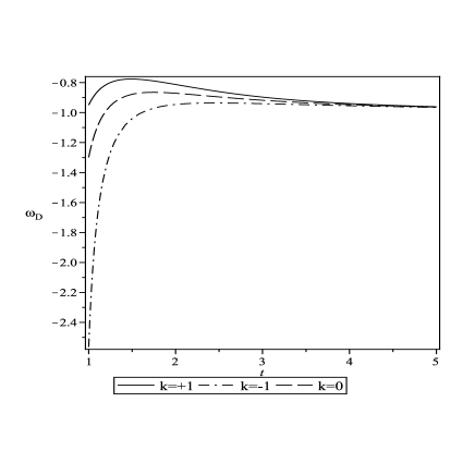
Figure 1: The plot of EoS parameter vs $t$ for $\rho_{0}=10$ and $\omega_{m}=0.5$

and

$$p_{D}=-\left(2\frac{\ddot{a}}{a}+\frac{\dot{a}^{2}}{a^{2}}+\frac{k}{a^{2}}\right)-\rho_{0}\omega_{m}a^{-3(1+\omega_{m})}.$$ (12)

Now we take following ansatz for the scale factor, where increase in term of time evolution

$$a(t)=\sqrt{te^{t}}.$$ (13)

The motivation to choose such scale factor is behind the fact that the universe is accelerated expansion at present and decelerated expansion in the past. Also, the transition redshift from deceleration expansion to accelerated expansion is about 0.5. Thus, in general, the DP is not a constant but time variable. By the above choice of scale factor yields a time dependent DP.

By using this scale factor in Eqs. (11) and (12), the $\rho_{D}$ and $p_{D}$ are obtained as

$$\rho_{D}=3\left[\frac{(1+t)^{2}}{4t^{2}}+\frac{k}{te^{t}}\right]-\rho_{0}(te^{t})^{-\frac{3}{2}(1+\omega_{m})},$$ (14)

and

$$p_{D}=-\left[\frac{3(1+t)^{2}-4}{4t^{2}}+\frac{k}{te^{t}}+\rho_{0}\omega_{m}(te^{t})^{-\frac{3}{2}(1+\omega_{m})}\right],$$ (15)

respectively. By using Eqs. (14) and (15) in Eq. (7), we find the equation of state of dark field in term of time as

$$\omega_{D}=-\left[\frac{\frac{3(1+t)^{2}-4}{4t^{2}}+\frac{k}{te^{t}}+\rho_{0}\omega_{m}(te^{t})^{-\frac{3}{2}(1+\omega_{m})}}{3\left[\frac{(1+t)^{2}}{4t^{2}}+\frac{k}{te^{t}}\right]-\rho_{0}(te^{t})^{-\frac{3}{2}(1+\omega_{m})}}\right].$$ (16)

The behavior of EoS for DE in term of cosmic time $t$ is shown in Fig.1. It is observed that although for open, close and flat universes the EoS parameter is an increasing function of time, the rapidity of its growth at the early stage depends on the type the universe. Later on it tends to the same constant value independent of the types of the universe.

The expressions for the matter-energy density $\Omega_{m}$ and dark-energy density $\Omega_{D}$ are given by

$$\Omega_{m}=\frac{\rho_{m}}{3H^{2}}=\frac{4t^{2}}{3(1+t)^{2}}\rho_{0}(te^{t})^{-\frac{3}{2}(1+\omega_{m})},$$ (17)

and

$$\Omega_{D}=\frac{\rho_{D}}{3H^{2}}=1+\frac{4kt}{3(1+t)^{2}e^{t}}-\frac{4t^{2}}{3(1+t)^{2}}\rho_{0}(te^{t})^{-\frac{3}{2}(1+\omega_{m})},$$ (18)

respectively. Equations (17) and (18) reduce to

$$\Omega=\Omega_{m}+\Omega_{D}=1+\frac{4kt}{3(1+t)^{2}e^{t}}.$$ (19)

From the right hand side of Eq. (19) it is clear that in flat universe ($k=0$), $\Omega=1$ and in open universe ($k=-1$), $\Omega<1$ and in close universe ($k=+1$), $\Omega>1$. But at late time we see for all flat, open and close universes $\Omega\to 1$. This result is compatible with the observational results. Since our model predicts a flat universe for large times and the present-day universe is very close to flat, the derived model is also compatible with the observational results. The variation of density parameter with cosmic time has been shown in Fig.2.

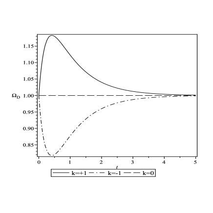
Figure 2: The plot of density parameter ($\Omega$) vs $t$ for $n=3$

We define the deceleration parameter $q$ as usual, i.e.

$$q=-\frac{\ddot{a}a}{\dot{a}^{2}}=-\frac{\ddot{a}}{aH^{2}}.$$ (20)

Using Eqs. (3) and (4), we may rewrite Eq. (20) as

$$q=\frac{1}{6H^{2}}\left[\rho_{m}(1+3\omega_{m})+\rho_{D}(1+3\omega_{D})\right].$$ (21)

On the other hand, using Eq. (13) into Eq. (20), we find

$$q=\frac{2}{(1+t)^{2}}-1.$$ (22)

From Eq. (22), we observe that $q>0~{}~{}\mbox{for}~{}t<0.41$ and $q<0~{}~{}\mbox{for}~{}t>0.41$. This behavior of $q$ is clearly depicted in Fig.3

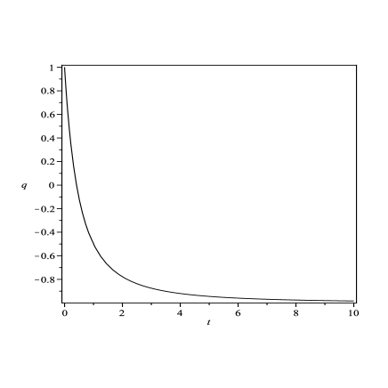
Figure 3: The plot of deceleration parameter ($\Omega$) vs $t$

A convenient method to describe models close to $\Lambda$ CDM is based on the cosmic jerk parameter $j$, a dimensionless third derivative of the scale factor with respect to the cosmic time [20]$-$[23]. A deceleration-to-acceleration transition occurs for models with a positive value of $j_{0}$ and negative $q_{0}$. Flat $\Lambda$ CDM models have a constant jerk $j=1$. The jerk parameter in cosmology is defined as the dimensionless third derivative of the scale factor with respect to cosmic time

$$j(t)=\frac{1}{H^{3}}\frac{\dot{\ddot{a}}}{a}.$$ (23)

and in terms of the scale factor to cosmic time

$$j(t)=\frac{(a^{2}H^{2})^{{}^{\prime\prime}}}{2H^{2}},$$ (24)

where the ‘dots’ and ‘primes’ denote derivatives with respect to cosmic time and scale factor, respectively. The jerk parameter appears in the fourth term of a Taylor expansion of the scale factor around $a_{0}$,

$$\frac{a(t)}{a_{0}}=1+H_{0}(t-t_{0})-\frac{1}{2}q_{0}H_{0}^{2}(t-t_{0})^{2}+\frac{1}{6}j_{0}H_{0}^{3}(t-t_{0})^{3}+O\left[(t-t_{0})^{4}\right],$$ (25)

where the subscript $0$ shows the present value. One can rewrite Eq. (23) as

$$j(t)=q+2q^{2}-\frac{\dot{q}}{H}.$$ (26)

Equations (22) and (26) reduce to

$$j(t)=\frac{t^{3}+3(t^{2}-t+1)}{(1+t)^{3}}.$$ (27)

This value overlaps with the value $j\simeq 2.16$ obtained from the combination of three kinematical data sets: the gold sample of type Ia supernovae [24], the SNIa data from the SNLS project [25], and the x-ray galaxy cluster distance measurements [26] at $t\simeq 0.05$.

4 Interacting two fluids model

Secondly, we consider the interaction between dark and barotropic fluids. For this purpose we can write the continuity equations for dark fluid and barotropic fluids as

$$\dot{\rho}_{m}+3\frac{\dot{a}}{a}\left(\rho_{m}+p_{m}\right)=Q,$$ (28)

and

$$\dot{\rho}_{D}+3\frac{\dot{a}}{a}\left(\rho_{D}+p_{D}\right)=-Q.$$ (29)

The quantity $Q$ expresses the interaction between the dark components. Since we are interested in an energy transfer from the dark energy to dark matter, we consider $Q>0$. $Q>0$ ensures that the second law of thermodynamics stands fulfilled [27]. Here we emphasize that the continuity Eqs. (28) and (29) imply that the interaction term ($Q$) should be proportional to a quantity with units of inverse of time. i.e $Q\propto\frac{1}{t}$. Therefore, a first and natural candidate can be the Hubble factor $H$ multiplied with the energy density. Following Amendola et al. [28] and Gou et al. [29], we consider

$$Q=3H\sigma\rho_{m},$$ (30)

where $\sigma$ is a coupling constant. Using Eq. (30) in Eq. (28) and after integrating the resulting equation, we obtain

$$\rho_{m}=\rho_{0}a^{-3(1+\omega_{m}-\sigma)}.$$ (31)

By using Eq. (31) in Eqs. (3) and (4), we again obtain the $\rho_{D}$ and $p_{D}$ in terms of scale factor $a(t)$.

$$\rho_{D}=3\left(\frac{\dot{a}^{2}}{a^{2}}+\frac{k}{a^{2}}\right)-\rho_{0}a^{-3(1+\omega_{m}-\sigma)},$$ (32)

and

$$p_{D}=-\left(2\frac{\ddot{a}}{a}+\frac{\dot{a}^{2}}{a^{2}}+\frac{k}{a^{2}}\right)-\rho_{0}(\omega_{m}-\sigma)a^{-3(1+\omega_{m}-\sigma)},$$ (33)

respectively. Putting the value of $a(t)$ from Eq. (13) in Eqs. (32) and (33), we obtain

$$\rho_{D}=3\left[\frac{(1+t)^{2}}{4t^{2}}+\frac{k}{te^{t}}\right]-\rho_{0}(te^{t})^{-\frac{3}{2}(1+\omega_{m}-\sigma)},$$ (34)

and

$$p_{D}=-\left[\frac{3(1+t)^{2}-4}{4t^{2}}+\frac{k}{te^{t}}+\rho_{0}\omega_{m}(te^{t})^{-\frac{3}{2}(1+\omega_{m}-\sigma)}\right],$$ (35)

respectively. Using Eqs. (34) and (35) in Eq. (7), we can find the EoS parameter of dark field as

$$\omega_{D}=-\left[\frac{\frac{3(1+t)^{2}-4}{4t^{2}}+\frac{k}{te^{t}}+\rho_{0}\omega_{m}(te^{t})^{-\frac{3}{2}(1+\omega_{m}-\sigma)}}{3\left[\frac{(1+t)^{2}}{4t^{2}}+\frac{k}{te^{t}}\right]-\rho_{0}(te^{t})^{-\frac{3}{2}(1+\omega_{m}-\sigma)}}\right].$$ (36)

The behavior of EoS in term of cosmic time $t$ is shown in Fig.4. It is observed that like the minimal coupling case, the EoS parameter is an increasing function of time for all close, open and flat universes, the rapidity of its increase at the early stage depends on the type of universe. At the later stage of evolution it tends to the same constant value independent of the types of the Universe. The EoS parameter of DE begins in phantom region and tends to $-1$ (cosmological constant.

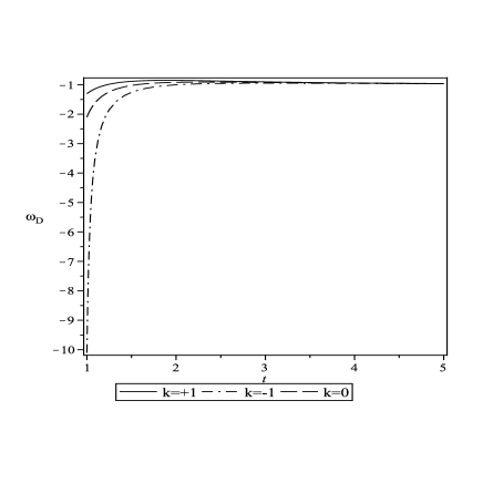
Figure 4: The plot of EoS parameter vs $t$ for $\rho_{0}=10,\omega_{m}=0.5$ and $\sigma=0.3$

The expressions for the matter-energy density $\Omega_{m}$ and dark-energy density $\Omega_{D}$ are given by

$$\Omega_{m}=\frac{\rho_{m}}{3H^{2}}=\frac{4t^{2}}{3(1+t)^{2}}\rho_{0}(te^{t})^{-3n(1+\omega_{m}-\sigma)},$$ (37)

and

$$\Omega_{D}=\frac{\rho_{D}}{3H^{2}}=1+\frac{4kt}{3(1+t)^{2}e^{t}}-\frac{4t^{2}}{3(1+t)^{2}}\rho_{0}(te^{t})^{-3n(1+\omega_{m}-\sigma)},$$ (38)

respectively. From Eqs. (37) and (38), we obtain

$$\Omega=\Omega_{m}+\Omega_{D}=1+\frac{4kt}{3(1+t)^{2}e^{t}},$$ (39)

which is the same as Eq. (19). Therefore, we observe that in the interacting case the density parameter has the same properties as in the non-interacting case. The expressions for deceleration parameter and jerk parameter are also the same as in the case of non-interacting case.

Studying the interaction between the dark energy and ordinary matter will open a possibility of detecting the dark energy. It should be pointed out that evidence was recently provided by the Abell Cluster A586 in support of the interaction between dark energy and dark matter [30, 31]. We observe that in the non-interacting case only open and flat universes can cross the phantom region whereas in interacting case all open, flat and close universes can cross phantom region.

5 Concluding Remarks

In summary, we have studied the system of two-fluid within the scope of a spatially flat and isotropic FRW model. The role of two-fluid minimally or directly coupled in the evolution of the dark energy parameter has been investigated. In doing so the scale factor is taken to be an exponential law function of time. It is concluded that in the non-interacting case only open and flat universes cross the phantom region whereas in the interacting case all three universes can cross the phantom region.

References

-
[1]
S. Perlmutter et al., Astrophys. J. 483, (1997) 565.
S. Perlmutter et al., Nature 391, (1998) 51.
S. Perlmutter et al., Astrophys. J. 517, (1999) 5. -
[2]
A. G. Riess et al., Astron. J. 116, (1998) 1009.
A. G. Riess et al., Publ. Astron. Soc. Pacific 112, (2000) 1284. -
[3]
P. M. Garnavich et al., Astrophys. J. 493, 1998 L53.
P. M. Garnavich et al., Astrophys. J. 509, (1998) 74.
- [4] B. P. Schmidt et al., Astrophys. J. 507, (1998) 46.
- [5] J. L. Tonry et al., Astrophys. J. 594, (2003) 1.
- [6] A. Clocchiatti et al., Astrophys. J. 642, (2006) 1.
- [7] P. de Bernardis et al., Nature 404, (2000) 955.
- [8] S. Hanany et al., Astrophys. J. 545, (2000) L53.
- [9] D. N. Spergel et al., Astrophys. J. Suppl. 148, (2003) 175.
- [10] M. Tegmark et al., Phys. Rev. D 69, (2004) 103501.
- [11] U. Seljak et al., Phys. Rev. D 71, (2005) 103515.
- [12] J. K. Adelman-McCarthy et al., Astrophys. J. Suppl. 162, (2006) 38.
- [13] C. L. Bennett et al., Astrophys. J. Suppl. 148, (2003) 1.
- [14] S. W. Allen et al., Mon. Not. R. Astron. Soc. 353, (2004) 457.
- [15] X. F. Zhang and H. H. Liu, Chin. Phys. Lett. 26, (2009) 109803.
- [16] N. M. Liang, C. J. Gao and S. N. Zhang, Chin. Phys. Lett. 26, (2009) 069501.
- [17] I. A. Arbab, Chin. Phys. Lett. 25, (2008) 3834.
- [18] C. Wang, Y. B. Wu and F. Liu, Chin. Phys. Lett. 26, (2009) 029801.
- [19] M. R. Setare, J. Sadeghi and A. R. Amani, Phys. Lett. B 673, (2009) 241.
- [20] Chiba T and Nakamura T 1998 Prog. Theor. Phys. 100, (1998) 1077.
- [21] V. Sahni, [arXiv:astro-ph/0211084] (2002).
- [22] R. D. Blandford, M. Amin, E. A. Baltz, K. Mandel and P. J. Marshall, [arXiv:astro-ph/0408279] (2004).
-
[23]
M. Visser, Class. Quantum Grav. 21, (2004) 2603.
M. Visser, Gen. Relativ. Gravit. 37, (2005) 1541. - [24] A. G. Riess et al., Astrophys. J. 607, (2004) 665.
- [25] P. Astier et al., Astron. Astrophys. 447, (2006) 31.
- [26] D. Rapetti, S. W. Allen, M. A. Amin and R. D. Blandford, Mon. Not. Roy. Astron. Soc. 375, (2007) 1510.
- [27] D. Pavon and B. Wang, Gen. Relativ. Gravit. 41, (2009) 1.
- [28] L. Amendola, G. Camargo Campos and R. Rosenfeld, Phys. Rev. D 75, (2007) 083506.
- [29] Z. K. Guo, N. Ohta and S. Tsujikawa, Phys. Rev. D 76, (2007) 023508.
- [30] O. Bertolami, F. Gil Pedro and M. Le Delliou, Phys. Lett. B 654, (2007) 165.
- [31] M. Le Delliou, O. Bertolami and F. Gil Pedro, AIP Conf. Proc. 957, (2007) 421, [arXiv:0709.2505 [astro-ph].