Density Estimation for Projected Exoplanet Quantities

Abstract

Exoplanet searches using radial velocity (RV) and microlensing (ML) produce samples of “projected” mass and orbital radius, respectively. We present a new method for estimating the probability density distribution (density) of the unprojected quantity from such samples. For a sample of $n$ data values, the method involves solving $n$ simultaneous linear equations to determine the weights of delta functions for the raw, unsmoothed density of the unprojected quantity that cause the associated cumulative distribution function (CDF) of the projected quantity to exactly reproduce the empirical CDF of the sample at the locations of the $n$ data values. We smooth the raw density using nonparametric kernel density estimation with a normal kernel of bandwidth $\sigma$. We calibrate the dependence of $\sigma$ on $n$ by Monte Carlo experiments performed on samples drawn from a theoretical density, in which the integrated square error is minimized. We scale this calibration to the ranges of real RV samples using the Normal Reference Rule. The resolution and amplitude accuracy of the estimated density improve with $n$. For typical RV and ML samples, we expect the fractional noise at the PDF peak to be approximately 80 $n^{-\log 2}$. For illustrations, we apply the new method to 67 RV values given a similar treatment by Jorissen et al. in 2001, and to the 308 RV values listed at exoplanets.org on 20 October 2010. In addition to analyzing observational results, our methods can be used to develop measurement requirements—particularly on the minimum sample size $n$—for future programs, such as the microlensing survey of Earth-like exoplanets recommended by the Astro 2010 committee.

1 INTRODUCTION

Mass $m$ and orbital radius $r$ are two key factors for the habitability of exoplanets. This is because $m$ plays an important role in the retention of an atmosphere, and $r$ is a key determinant of the surface temperature. Besides those connections to the cosmic search for life, the true distributions of $m$ and $r$ are also important for theories of the formation and dynamical evolution of planetary systems. Therefore, we have a variety of good reasons to better understand the cosmic distributions of $m$ and $r$. Such improvement will involve learning more from measurements already made, as well as anticipating results from the telescopes and observing programs of the future.

We focus on two astronomical techniques that measure projected planetary quantities. One is radial velocity (RV), the source of many exoplanet discoveries so far. The other is microlensing (ML). Astro 2010 recently recommended a ML survey for Earth-mass exoplanets on orbits wider than detectable by Kepler (Blandford et al. 2010).

RV yields the unprojected value of $r$, from the observed orbital period and an estimate of the stellar mass, but for mass it can only provide $m\sin i$—not $m$—where $i$ is the usually unknown orbital inclination angle. Correspondingly, if the mass of the lens and the stellar distances are known or assumed, ML yields $m$, but for $r$ it usually can provide only $r\sin\beta$—not $r$—where $\beta$ is the usually unknown planetocentric angle between the star and observer (Gaudi 2011). For the foreseeable future, only an ML survey appears to offer observational access to exoplanets like Earth in mass and orbital radius around Sun-like stars. A high-confidence estimate of the occurrence probability of such planets around nearby stars is critical to designing future telescopes to obtain their spectra and search for signs of life.

Even when the projection angle $\beta$ is unknown, we can use statistical methods to draw inferences from samples of the projected values about the distribution of the true, unprojected values in nature. This paper presents a new method to help draw those inferences.

One goal of this paper is to introduce a science metric for the ML survey, and to demonstrate its use with existing RV results. The ML metric is the resolution and accuracy of the estimated probability density of the orbital radii of Earth-mass exoplanets. Such a science metric will be useful for setting measurement requirements, designing telescopes and instruments, planning science operations, and arriving at realistic expectations for the new ML survey program.

2 STARTING POINT

Our starting point is recognizing that the projected quantity, $\varphi\equiv m\sin i$ or $r\sin\beta$, is the product of two independent continuous random variables, $\rho\equiv m$ or $r$, and $y\equiv\sin i$ or $\sin\beta$, which have densities $\Psi(\rho)$ and ${\cal Q}(y)$, respectively. Assuming the directions of planetary radius vectors and orbital poles are uniformly distributed on the sphere,

$${\cal Q}(y)=\frac{y}{\sqrt{1-y^{2}}}~{}~{}.$$ (1)

$\rho$ and $y$ have ranges $0\leq\rho\leq\infty$ and $0\leq y\leq 1$. The product $\varphi=\rho y$ is also a random variable, with the density $\Phi(\varphi)$, which we can calculate as follows. The probability density at a point $\{{\rho,y}\}$ on the $\rho$–$y$ plane—within the ranges of $\rho$ and $y$—is $\Psi(\rho)\;{\cal Q}(y)$, and $\Phi(\varphi)$ is the integral of this product over the portion of the $\rho$–$y$ plane where $\rho y=\varphi$:

$$\Phi(\varphi) = \int_{0}^{\infty}{\int_{0}^{1}{\Psi(\rho){\cal Q}(y)}}\delta_{\varphi}(\rho y-\varphi)dy\,d\rho$$

$$= \int_{0}^{\infty}{\Psi(\rho)\int_{0}^{1}{{\cal Q}(y)}}\delta_{y}\left({y-\frac{\varphi}{\rho}}\right)\frac{1}{\rho}dy\,d\rho$$

$$= \int_{\varphi}^{\infty}{\Psi(\rho){\cal Q}\left({\frac{\varphi}{\rho}}\right)}\frac{1}{\rho}\,d\rho~{}~{},$$

where $\delta_{z}$ is the Dirac delta function for any variable $z$, with the normalization

$$\int_{-\infty}^{\infty}{\delta_{z}(z-a)dz=1}~{}~{},$$ (3)

and where in the last line of Eq. 2 we have used the fact that $\rho$ must always be greater than $\varphi$. We now change the variable $\varphi\to u\equiv\log\varphi$ with the density ${\cal P}(u)$:

$${\cal P}(u) = \Phi(\varphi)\frac{d\varphi}{du}=\Phi({10^{u}})(\ln 10)10^{u}$$ (4)

$$= ({\ln 10})10^{u}\int_{10^{u}}^{\infty}{\Psi(\rho){\cal Q}\left({\frac{10^{u}}{\rho}}\right)}\frac{1}{\rho}\,d\rho~{}~{}.$$

We now change the variable $\rho\to x\equiv\log\rho$, with the density ${\cal R}(x)$. Using the relation $\Psi(\rho)\,d\rho={\cal R}(x)\;dx$, we have

$${\cal P}(u)={\cal C}(u)({\ln 10})\int_{u}^{\infty}{{\cal R}(x){\cal Q}({10^{u-x}})}10^{u-x}dx~{}~{}.$$ (5)

In Eq. 5, we have introduced a new factor, the completeness function ${\cal C}(u)$, to account for variations in search completeness due to, for example, the variation of instrumental sensitivity with $u$. The clearest example is declining signal-to-noise ratio with smaller $u$—smaller $m\sin i$ in the case of RV and smaller $r\sin\beta$ for ML. In this paper, we ignore completeness effects and assume ${\cal C}(u)\equiv 1.$ In the case of the density estimation studies in Section 4, this means we have not necessarily chosen a realistic theoretical ${\cal R}(x)$, but realism is probably not necessary for the immediate purposes—achieving a valid calibration of the bandwidth (smoothing length) $\sigma$ and exploring resolution and accuracy. In the case of the analysis of real RV data in Section 5, we need only to remember that scientific interpretations of the distributions we infer for ${\cal R}(\log m)$ will demand qualification regarding the potential effects of ${\cal C}(u)$, particularly for the left-hand tails of the distribution, where incompleteness due to low signal-to-noise ratio must be important.

We recognized that Eq. (5) has a thought-provoking analogy to the case of an astronomical image (which corresponds to ${\cal P}$), where the object (${\cal R})$ is convolved with the telescope’s point-spread function (${\cal Q}$) and the field is, say, vignetted in the camera (${\cal C}$). Pursuing this analogy, we might call the form of the integral in Eq. (2) “logarithmic convolution.” It could be said that we “see” the true distribution (${\cal R}$) only after it has been logarithmically convolved with the projection function (${\cal Q}$) and modulated by the completeness function (${\cal C}$). As with image processing, we can correct “vignetting” by dividing ${\cal P}$ by ${\cal C}$, if we know it, and then “deconvolve” the result to remove the effects of ${\cal Q}$—which in this case we know exactly. As with image processing, the result can be a transformation—a new, alternative, precise description of the sample, in the form of an estimate of the “object,” the natural density ${\cal R}$, with some systematic effects reduced or removed (but other effects possibly remaining).

Equation (5) is a form of Abel’s integral equation, as discussed in this general context by Chandrasekhar & Münch (1950), who used the formal solution to investigate the distribution of true and apparent rotational velocities of stars. Later, Jorissen et al. (2001) inferred the distribution of exoplanet masses from 67 values of $m\sin i$, using both the formal solution and the Lucy-Richardson algorithm, which is an implementation of the expectation-maximization algorithm that is widely used in maximum-likelihood estimation (Dempster et al. 1977). We present a third numerical approach to solving Eq. (5).

In Section 3, we develop the new method for transforming samples of measured values into a raw, unsmoothed density for $x$. In Section 4, we discuss nonparametric density estimation, random deviates, and the qualitative accuracy of the estimated density. In Section 5, we illustrate these computations on samples of RV results—the 67 values treated by Jorissen et al. (2001) and the 308 values of $m\sin i$ available at exoplanets.org on 20 October 2010. In Section 6, we comment on implications and future directions.

3 NEW METHODS

We assume the sample of independent and identically distributed, projected values $\{u\}$ is non-redundant and sorted in ascending order. The cardinality of the sample is $n$. The empirical cumulative distribution function (CDF) for $u$ is

$$\hat{P}(u)\equiv\frac{1}{n}\sum\nolimits_{i=1}^{n}{\cal I}(u_{i}\leq u)~{}~{},$$ (6)

where ${\cal I}$ is the indicator function

$${\cal I}(\mathit{logical\ statement})\equiv 1\ \mathrm{if\ the\ statement\ is\ true\ and\ 0\ otherwise}.$$ (7)

$\hat{P}$ estimates the true CDF of the projected quantity, which is

$$P(u)\equiv\int_{-\infty}^{u}{\cal P}(u^{\prime})du^{\prime}~{}~{}.$$ (8)

We can approximate ${\cal R}$ by a sum of Dirac delta functions at $N$ points $\{x\}$ with weights $\{w\}$:

$${\cal R}(x)\simeq\hat{\cal R}(x)\equiv\sum\nolimits_{j=1}^{N}w_{j}\delta(x-x_{j})~{}~{}.$$ (9)

The associated approximation of $P(u)$ is

$$P(u)\simeq\hat{P}^{\prime}(u) \equiv \int_{-\infty}^{u}{\ln 10\int_{{u}^{\prime}}^{\infty}{\sum\nolimits_{j=1}^{N}{w_{j}\delta(x-x_{j})}{\cal Q}(10^{{u}^{\prime}-x})}10^{{u}^{\prime}-x}dxd{u}^{\prime}}$$

$$= \sum\nolimits_{j=1}^{N}{w_{j}\ln 10\int_{-\infty}^{u}{\frac{10^{2({u}^{\prime}-x_{j})}}{\sqrt{1-10^{2({u}^{\prime}-x_{j})}}}}}{\cal H}(-{u}^{\prime}+x_{j})d{u}^{\prime}$$

$$= \sum\nolimits_{j=1}^{N}{w_{j}\left({1-\sqrt{1-10^{2(u-x_{j})}}{\cal H}(-u+x_{j})}\right)}~{}~{},$$

where

$${\cal H}(-a+b)\equiv 1\mbox{ if }a\leq b\mbox{ and }0\mbox{ if }a>b$$ (11)

is the Heaviside unit-step function. When we set $N=n$, $u=u_{i}$, and $x_{j}$, the critically determined set of linear equations

$$\sum\nolimits_{j=1}^{N}{w_{j}\left({1-\sqrt{1-10^{2(u_{i}-u_{j})}}H(-u_{i}+u_{j})}\right)}=\frac{1}{n}\sum\nolimits_{k=1}^{n}I(u_{k}\leq u_{i})$$ (12)

can be solved for $\{w\}$ by multiplying the vector that is the right side of Eq. (12) by the inverse of the matrix that is the outer parentheses on the left side.

The resulting estimates of the raw, unsmoothed density and CDF of $x$ are $\hat{\cal R}(x)$ in Eq. (9) and

$$\hat{R}(x)\equiv\sum\nolimits_{j=1}^{N}{w_{j}{\cal H}(x-x_{j})}~{}~{},$$ (13)

respectively. $\hat{P}(u)$ and ${\hat{P}}^{\prime}(u)$ produce identical results when evaluated at the sample points $\{u\}$. We recognize that they are not estimates but pure transformations of the sample, through the intermediary of the weights $\{w\}$. The same is true of $\hat{\cal R}$ and $\hat{R}$, which are sums of discontinuous functions. Indeed, the sum of delta functions in Eq. (9) is not particularly useful in itself because it conveys nothing more than the transformed sample. We must smooth $\hat{\cal R}_{(}x)$ in order to calculate non-zero results for the density at values of the unprojected quantity other than the sample points. We discuss this smoothing in the next section.

4 NONPARAMETRIC DENSITY ESTIMATION

Here we explore the issues associated with smoothing the raw density, $\hat{\cal R}(x)$. Without smoothing, the form of $\hat{\cal R}(x)$ in Eq. (9) is not very interesting or useful, because the only values it takes on are plus and minus infinity and zero. In order to pursue practical research with $\hat{\cal R}(x)$—such as comparing observations with theories, learning about possible variations of ${\cal R}(x)$ with other planetary or stellar parameters, and informing the measurement requirements for future missions and observing programs—we need $\hat{\cal R}(x)$ in the form of a sufficiently smoothed positive function. At the same time, we want to avoid over-smoothing, which might discard real detail.

The astronomer s “smoothing” is called “nonparametric density estimation” in statistics and other fields (see Silverman 1986, Takezawa 2006, and Wasserman 2006). Our approach, of convolving the raw density with a Gaussian of standard deviation $\sigma$,

$$\hat{\cal R}_{\sigma}(x)=\sum\nolimits_{i=1}^{m}w_{j}\frac{1}{\sqrt{2\pi}\sigma}e^{-\frac{(x-u_{i})^{2}}{2\sigma^{2}}}~{}~{},$$ (14)

is called “kernel density estimation with a normal kernel of bandwidth $\sigma$.” The standard statistical treatment flows from the study of histograms of samples of independent, identically distributed random variables, in the limit as (a) the bin width tends to zero, (b) the count in any bin becomes zero or one, (c) the raw density is the sum of delta functions of equal, positive weight (1/$n$) located at the sample points, and (d) the kernel density estimate is the sum of identical kernel functions located at the sample points. Ours is a different case, for which a theory must still be developed. Our raw density [Eq. (9)] is the sum of unequally weighted delta functions, and the weights include both positive and negative values. These differences from the standard case occur because we are estimating density in the unprojected space—where the sample is represented by the unequal, positive and negative weights—rather than in the projected space of the sample itself.

A considerable literature has been developed on the tasks of selecting the kernel and bandwidth for the standard case. Optimizing the bandwidth usually calls for defining an objective function (figure of merit), which is maximized or minimized. Because the true density is not known, by definition, the objective function must be computed from the sample and bandwidth alone. It is not immediately clear how the extensive work on this problem in the standard case applies to the current case. Therefore, we take an empirical approach to bandwidth selection for a normal kernel by conducting Monte Carlo experiments with a theoretical true density.

We expect the optimal value of $\sigma$ to be well-defined, because the asymptotes of Eq. (14) are trivial: reversion to Eq. (9) for $\sigma\rightarrow 0$ and approaching zero everywhere as $\sigma\rightarrow\infty$. Therefore, the optimal value of $\sigma$ must lie in between. In addition, we expect the optimal value to decrease with higher cardinality of the sample, $n$, because the increased information from more observations should include more information about detail. At least for $\sigma\ll\Delta u$, the metric for the range of $u$, we expect by simple scaling that the optimal value of $\sigma$ for different problems is proportional to $\Delta u$. Following Wasserman (2006; p. 135), we measure the range using the range metric in the Normal Reference Rule: $\Delta u\equiv\min(s,q/1.34)$, where $s$ is the sample standard deviation and $q$ is the interquartile range.

As a first exploration, we study the case of a theoretical density ${\cal R}(x)$ comprising three Gaussians, with $\{$mean, standard deviation, weight$\}=\{0.5,0.25,2.0\}$, $\{2.0,0.5,8.0\}$, and $\{2.5,0.125,1.0\}$. In this case, $\Delta u=0.783$. For this exercise we developed a facility to perform the following sequence of steps: (1) create random samples $\{u\}$ of cardinality $n$, where each value is drawn from the random deviate or $u$; and for such samples, (2) solve Eqs. (12) for weights $\{w\}$; (3) construct the estimated density $\hat{\cal R}_{\sigma}(x)$ for any value of $\sigma$ using Eq. (14); (4) compute the objective function (integrated square error) $v$ for the closeness of $\hat{\cal R}_{\sigma}(x)$ to ${\cal R}(x)$ , where

$$v\equiv\int_{-\infty}^{\infty}\left(\hat{\cal R}_{\sigma}(x)-{\cal R}(x)\right)^{2}dx~{}~{};$$ (15)

and (5) determine the value of $\sigma$ that minimizes $v$, which we adopt as the working definition of the optimal value of $\sigma$.

The random deviate for $u$ is

$$\mathbb{U}=\log(10^{\mathbb{X}}\mathbb{Y})~{}~{},$$ (16)

where

$$\mathbb{X}=x\mathrm{-root}\left(\int_{-\infty}^{x}R(x^{\prime})dx^{\prime}=\mathbb{Z}\right)~{}~{},$$ (17)

where $R(x^{\prime})$ stands for the true or estimated density under study, where

$$\mathbb{Y}=\sqrt{2\mathbb{Z}-\mathbb{Z}^{2}}~{}~{},$$ (18)

where $\mathbb{Z}$ is the uniform random deviate on the range 0–1, and where “$x$-root” in Eq. (17) is defined as the value of $x$ that satisfies the equation in parenthesis.

The results of experiments involving these five steps are shown in Figs. 1–6. Figure 1 confirms the expectation that lower values of $\sigma$ retain the spiky original pattern of delta functions in Eq. (9), and that higher values of $\sigma$ reduce contrast by blurring features. As suggested by the progression of the colored curves in Figure 1, varying $\sigma$ to minimize $v$ will work efficiently to locate an optimal value, which for $n=100$ should be somewhere in the range $0.1<\sigma<0.4$.

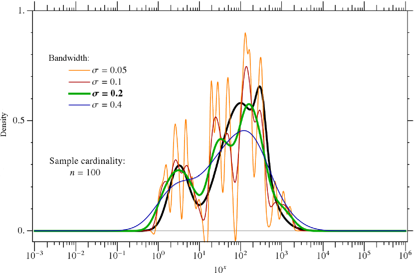
Figure 1: For a theoretical three-Gaussian density ${\cal R}(x)$ (black curve), the effects of convolving the raw density $\hat{\cal R}(x)$ with normal kernels of various bandwidths $\sigma$. Four random samples $\{u\}$ with $n=100$ were prepared using Eq. (4). The four sets of weights $\{w\}$ were determined by solving Eqs. (12). The four functions $\hat{\cal R}(x)$ resulting from Eq. (9) produced four functions $\hat{\cal R}_{\sigma}(x)$ from Eq. (14) with $\sigma=0.05$, 0.10, 0.2, and 0.4, which are plotted here in color. The red and orange curves are under-smoothed and still dominated by vestiges of the delta functions. The blue curve is over-smoothed: the dip between the two main peaks is blurred away, and the tails extend well beyond the range of ${\cal R}(x)$. The green curve is the most satisfactory of the four, accurately locating the two main peaks in ${\cal R}(x)$ and revealing the distinct minimum between them.

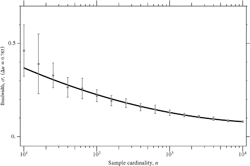
Figure 2: Bandwidth calibration, $\sigma(n)$. Points: mean values of $\sigma$ that minimize the integrated square error, determined from 24 samples $\{u\}$ for each value of $n$. Error bars: the standard deviations of the 24 values contributing to each mean. Curve: the weighted quadratic fit to the data points. We use this calibration, scaled by the range metric, to select $\sigma$ for all smoothing in the remainder of this paper.

Figure 2 shows the results of minimizing $v$ to optimize $\sigma$. For each of 16 values of $\log n$ in the range 1–4, we prepared 24 random samples $\{u\}$ of cardinality $n$, drawing from the same three-Gaussian distribution. Next, we adjusted $\sigma$ to minimize $v$ in order to obtain the optimal value of $\sigma$ for each sample. Next, we determined the mean and standard deviation of the 24 values of optimized $\sigma$ at each value of $n$. Finally, we computed the best quadratic fit to these data points, which is

$$\sigma(n)=\left(0.56-0.21\log n+0.023(\log n)^{2}\right)\frac{\Delta u}{0.783}~{}~{}.$$ (19)

We use Eq. (19) to compute the value of $\sigma$ in the remainder of this paper.

Figures 3–6 illustrate the qualitative improvement in the resolution and accuracy of the amplitudes of $\hat{\cal R}_{\sigma(n)}(x)$ as $n$ increases. In this controlled experiment, with ${\cal R}(x)$ known, we can evaluate performance in two ways: absolutely, by directly comparing $\hat{\cal R}_{\sigma(n)}(x)$ to the known ${\cal R}(x)$, and relatively, by assessing the variation of independent realizations of $\hat{\cal R}_{\sigma(n)}(x)$ with respect to each other. In this experiment, these alternative evaluations are shown to be consistent: features that repeat robustly in multiple realizations are seen to correspond to true characteristics of ${\cal R}(x)$. Meanwhile, features that do not repeat are spurious. Said differently, we find no robustly repeated features in $\hat{\cal R}_{\sigma(n)}(x)$ that are not present in ${\cal R}(x)$, nor any evidence that $\hat{\cal R}_{\sigma(n)}(x)$ with sufficiently high $n$ would fail to reproduce—to any desired accuracy—any feature in ${\cal R}(x)$, no matter how narrow or small in amplitude.

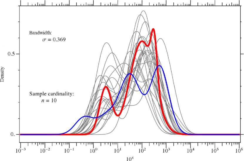
Figure 3: The variation of $\hat{\cal R}_{\sigma}(x)$ for $n=10$, in the case of the same theoretical three-Gaussian distribution ${\cal R}(x)$ (red curve). Gray and blue curves: 25 independent, random realizations of $\hat{\cal R}_{\sigma(n)}(x)$. There are no robustly repeated features in the recovered density that are present in the true density, except the extent and perhaps the skewness of ${\cal R}(x)$. This result suggests that RV or ML samples with $n=10$ over a comparable range should offer little information about the true distribution of mass or orbital radius. The fractional amplitude noise at the peak is about $\pm$40%.

In Figure 3, we find that samples with $n=10$ offer little information about the true distribution of $x$, with fluctuations on the scale of $\sim$40% amplitude near the peak. In Figure 4, we find that samples with $n=100$ offer crude information about the shape of the true distribution, with fluctuations on the scale of $\sim$20% amplitude near the peak. In Figure 5, we find that samples with $n=1000$ reveal the basic structure of the true distribution, with fluctuations on the scale of $\sim$10% amplitude near the peak. In Figure 6, resolution has improved, noise has been reduced, and some substructure is revealed, with fluctuations on the scale of $\sim$5% amplitude near the peak.

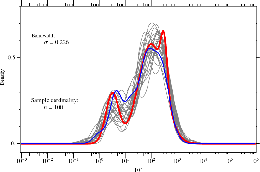
Figure 4: The variation of $\hat{\cal R}_{\sigma}(x)$ for $n=100$. Amplitude variation is reduced and resolution is increased. The bimodal character of ${\cal R}(x)$ is revealed. We see that RV or ML samples with $n=100$ should contain crude information about the shape of the true distribution of mass or orbital radius. The fractional amplitude noise at the peak is about $\pm$20%.

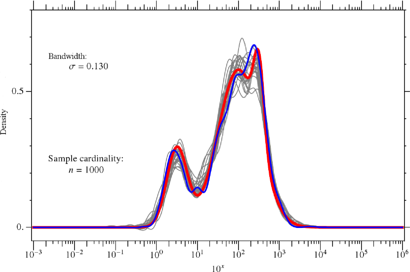
Figure 5: The variation of $\hat{\cal R}_{\sigma}(x)$ for $n=1000$. The locations and amplitudes of the two main peaks are accurately recovered. Improved resolution reveals the greater width of the right-hand peak compared with the left-hand peak, but the dip at the top is not recovered. Amplitude variation is further reduced. We find that RV or ML samples with $n=1000$ should convey information about the basic structure of the true distribution of mass or orbital radius, but would not reveal secondary features with less than about 10% amplitude, which is approximately the fractional noise amplitude at the peak.

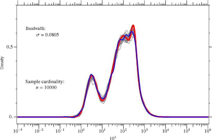
Figure 6: The variation of $\hat{\cal R}_{\sigma}(x)$ for $n=10,000$. The amplitude accuracy and resolution of individual realizations are further improved, and the small dip at the top of the right peak is marginally resolved. The fraction amplitude of noise at the peak is about $\pm$5%.

We can summarize these experiments with the finding that the fractional noise fluctuations at the peak, expressed as a percentage of the peak height, are approximately 80 $n^{-\log 2}$.

In the following section, we study real data from RV programs, where the true function ${\cal R}(x)$ is unknown—and indeed is the main object of the research. We require a method to determine which features are believable in the density $\hat{\cal R}_{\sigma(n)}(x)$ estimated from such data. For this we need the functional equivalent of a density of densities, to describe the distribution of $\hat{\cal R}_{\sigma(n)}(x)$, which is the distribution we might estimate from multiple, statistically equivalent data sets drawn from nature—but which we do not have, of course. The way forward is to assume that the unobtainable distribution is approximately the same as the distribution of functions $\hat{\cal R}_{\sigma(n)}(x)$ that we can compute from multiple samples drawn from the random deviate for the density $\hat{\cal R}_{\sigma(n)}(x)$ derived from the real data.

Basically, this approach uses self-consistency as a measure of the fidelity of the inferred density. It assumes that $\hat{\cal R}_{\sigma(n)}(x)$ is the true density and asks whether new, random data sets drawn from $\hat{\cal R}_{\sigma(n)}(x)$, with the same cardinality, robustly repeat the features in $\hat{\cal R}_{\sigma(n)}(x)$. If so, they are probably real. If not, they are probably spurious.

This approach to “confidence” in $\hat{\cal R}_{\sigma(n)}(x)$ is a natural extension of the Monte Carlo methods for determining confidence regions described in Section 14.5 of Press et al. (1986). We take this approach in the next section, where we study two real samples of RV data.

5 RV DATA

To illustrate the method developed in Sections 3–4, we treat two samples of RV data. The first is the 67 values of $m\sin i$ treated by Jorissen et al.  (2001), which were kindly provided to us by A. Jorissen. This sample is of particular interest because the authors used it to estimate the density for $m$ using Eq. (5) (which is identical to their Eq. 4 if completeness is ignored [$C(u)\equiv 1$] and the logarithmic variables are changed back to $m$ and $m\sin i$). Therefore, we can compare results.

Figure 7 shows our result for $\hat{\cal R}_{\sigma(n)}(\log m$), which is nearly featureless, unlike the Jorissen et al. results, shown in their Fig. 2. Because they do not use logarithmic variables, their results are simplified for $m<1.\,m_{\mathrm{J}}$, even though 31% of the sample values lie in that range. Nevertheless, we can recover the main features in the Jorissen et al. PDF for $m>1.\,m_{\mathrm{J}}$ if we grossly under-smooth.

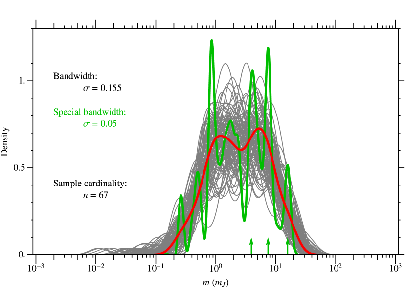
Figure 7: Treatment of the 67 RV data points of Jorissen et al. (2001). The value $\sigma=0.155$ comes from Eq. (19) using $\Delta u=0.491$, the range metric of the data. In red, the inferred metric, $\hat{\cal R}_{\sigma(n)}(\log m$). In gray, the confidence region delineated by densities generated from 100 statistically equivalent data sets drawn from the random deviate for $\hat{\cal R}_{\sigma(n)}(\log m$). The dip in the peak of the red curve is not believable, given the significantly greater width of the confidence region (gray). In green, an under-smoothed version of $\hat{\cal R}_{\sigma}(\log m$), with $\sigma=0.05$, which resembles the density inferred by Jorissen et al. (2001), for $m>1\,m_{\mathrm{J}}$, shown in their Fig. 2, particularly the peaks at $\sim$4.0, 7.5, and 15 $m_{\mathrm{J}}$, indicated here by green arrows. These features are apparently artifacts of under-smoothing.

The feature Jorissen et al. found most believable is the minimum between the second and third peaks (green arrows), in the range 10–13 $m_{\mathrm{J}}$. They applied a “jackknife” test and concluded that this minimum was a “robust result, not affected by the uncertainty in the solution.” Based on our experiments in Section 4, and on our treatment of the Jorissen data (red and gray in Fig. 7), all the features in our under-smoothed $\hat{\cal R}_{\sigma(n)}(\log m$), including the minimum favored by Jorissen et al., which we can reproduce, are artifacts of under-smoothing and spurious.

The dip in the peak of the red curve in Figure 7 is not believable, given the significantly greater width of the confidence region (gray).

The second sample we studied is the 308 values of $m\sin i$ listed at exoplanets.org on 20 October 2010. This sample is documented in Table 1, and Figure 8 shows the results of our treatment. The feature favored by Jorissen et al. at 10–13 $m_{\mathrm{J}}$ is also not present in this density, which is improved in both resolution and amplitude accuracy compared with $n=67$.

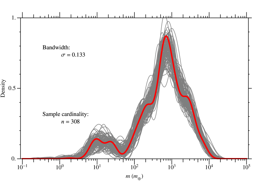
Figure 8: Treatment of the sample of 308 values of $m\sin i$ from RV observations listed at exoplanets.org on 20 October 2010. The sample is documented in Table 1. The value $\sigma=0.133$ comes from Eq. (19) using $\Delta u=0.600$, the approximate range of the data. In red, the inferred density, $\hat{\cal R}_{\sigma(n)}(\log m$). In gray, the confidence region delineated by densities generated from 100 statistically equivalent data sets, which were drawn from the random deviate for $\hat{\cal R}_{\sigma(n)}(\log m$). The rise of the density with decreasing $m$ from $\sim$50–10 $m_{\oplus}$ (0.16–0.03 $m_{\mathrm{J}}$) repeats robustly and is statistically significant.

For the $n=308$ density, the increase as $m$ decreases from $\sim$50 to $\sim$10 $m_{\oplus}$ (0.16–0.03 $m_{\mathrm{J}}$) repeats robustly in Monte Carlo trials and is statistically significant. Interestingly, this minimum is near the low-$m$ cutoff of the Jorissen data, and therefore no information about the bimodal character of $\hat{\cal R}_{\sigma(n)}(x)$ is present in the earlier sample of $n=67$ RV data points.

6 COMMENTS AND FUTURE DIRECTIONS

This paper offers an improved understanding of statistical inferences regarding the density of the unprojected quantities—mass $m$ for RV or radial distance $r$ for ML—from samples of the projected quantities, $m\sin i$ or $r\sin\beta$. The same treatment applies to both ML and RV.

We find that that ability to confidently recognize real features in the estimated density—and to reject spurious ones—depends on (1) the scale of the variations compared with the blurring scale of ${\cal Q}$ (standard deviation of 0.18 in the logarithm), (2) $\Delta u$, the metric of the range of the measurements, (3) the amplitudes of the features, and (4) $n$, the cardinality of the sample. The latter is the only factor controlled by the observer or the design of a mission.

Care must be given to the completeness factor, ${\cal C}(u)$, as well as to other possible systematic effects and biases that might affect the fidelity with which a sample of projected values reflects the true distribution of the unprojected quantity. For example, in the case of RV, we know that the detection efficiency—and therefore the completeness—decreases to zero as the projected mass—and therefore the signal-to-noise ratio ($u$ divided by the noise amplitude) decreases. Also, the least-squares estimator for mass from astrometry is known to be biased at low signal-to-noise ratio, and the same can be expected for $m\sin i$ from RV, as the treatment of all Keplerian signals is basically the same for planet detection by periodogram. (Brown 2009; see also Hogg et al. 2010) Any such factors affecting ML samples also bear close scrutiny. Monte Carlo experiments with the random deviates and analytic method developed in this paper should be helpful for studying the systematic effects of ${\cal C}(u)$ on the density.

Astro 2010 recommended an unbiased census of Earth-like exoplanets by WFIRST using the ML technique. This recommendation implies specific—but not yet defined—science requirements on the accuracy of the $\hat{\cal R}_{m}(r)$ inferred from ML events by exoplanets with typical characteristics $m\approx 1\,m_{\oplus}$ and $r\approx 1$ AU. In turn, these science requirements will imply measurement requirements—particularly on $n$, which controls random errors, and on knowledge of ${\cal C}(u)$, which controls systematic errors. In turn, the measurement requirements will flow down to the mission design, including both spacecraft and ground operations. We expect that Monte Carlo studies based on the method in this paper will be helpful in achieving adequacy and self consistency for the ML components of the WFIRST project, from spacecraft to ground operations.

We note that in the usual case where the angular factor $y$ is not known independently, Ho and Turner (2011) have recently pointed out that one must assume a density for the unprojected quantity $x$ in order to properly state the confidence interval for the value of $x$ derived from any particular observation of the projected quantity $u$. This is because the posterior distribution of $y$ is not the same as the prior distribution of $y$. The needed density could come from (1) a theoretical guesstimate (entailing systematic uncertainties), (2) a sample of $x$ from planets with known $y$ (transiting planets in the case of RV), or (3) a sample of $u$ from planets with unknown $y$, using the method developed in this paper.

The introduction of the logarithmic variables $u$, $x$, and $\log y$ in Section 2,

$$u=x+\log y~{}~{},$$ (20)

changed the problem from one of a product of random variables to one of a sum of random variables. This change creates a connection to recent statistical research on the “errors-in-variables” problem (Studenmayer et al. 2008; Apanasovich et al. 2009; Delaigle et al. 2009). The goal in this problem is to estimate the density of $x$, which is not observable, from observations of $u$, which is a version of $x$ contaminated by the additive, homoscedastic measurement error, $\log y$, with known density. The cited papers explore non-parametric estimation of the density of $x$ variously using B splines, simulation extrapolation, and local-polynomials. We expect that future research into density estimation for $m$ or $r$ from RV and ML samples of $m\sin i$ or $r\sin\beta$ will explore such advances in statistical research, and produce instructive comparisons with our approach—kernel density estimation with a normal kernel.

Table 1: The 308 Values of $m\sin i$ from RV at exoplanets.org on 20 October 2010

Exoplanet	$m\sin i(R_{\oplus})$		Exoplanet	$m\sin i(R_{\oplus})$		Exoplanet	$m\sin i(R_{\oplus})$
GJ 581 e	01.943		HD 45364 b	059.490		47 UMa c	173.489
HD 40307 b	04.103		HD 107148 b	067.444		HD 175541 b	182.742
HD 156668 b	04.151		HD 46375 b	072.222		HIP 14810 d	184.560
61 Vir b	05.110		HD 3651 b	072.786		HD 27894 b	196.424
GJ 581 c	05.369		HD 76700 b	073.793		HD 11964 b	196.508
GJ 876 d	05.893		HD 168746 b	077.913		GJ 876 c	196.761
HD 215497 b	06.629		HD 16141 b	079.359		HD 330075 b	198.268
HD 40307 c	06.722		HD 108147 b	082.012		HD 37124 d	202.306
GJ 581 d	07.072		HD 109749 b	087.311		HD 192263 b	203.245
HD 181433 b	07.544		HIP 57050 b	094.643		HD 181433 c	203.574
HD 1461 b	07.630		HD 101930 b	095.105		GJ 832 b	204.802
55 Cnc e	07.732		HD 88133 b	095.187		HD 216770 b	205.644
GJ 176 b	08.264		GJ 649 b	103.419		HD 37124 b	206.867
HD 40307 d	09.100		HD 215497 c	104.113		HD 45364 c	209.326
HD 7924 b	09.256		BD $-$08 2823 c	104.296		HD 170469 b	212.557
HD 69830 b	10.060		HD 33283 b	104.954		$\upsilon$ And b	212.747
61 Vir c	10.609		HD 47186 c	110.712		HD 96167 b	217.609
$\mu$ Ara d	10.995		HD 164922 b	113.777		HD 209458 b	218.862
GJ 674 b	11.087		HD 149026 b	114.129		HD 37124 c	221.403
HD 69830 c	11.689		HD 93083 b	117.035		HD 9446 b	222.123
BD $-$08 2823 b	14.604		HD 181720 b	118.247		HD 224693 b	227.153
HD 4308 b	15.175		HD 63454 b	122.451		HD 34445 b	239.582
GJ 581 b	15.657		HD 126614 A b	122.607		HD 187085 b	255.476
HD 69830 d	17.908		HD 83443 b	125.835		HD 134987 c	255.868
HD 190360 c	18.746		HD 212301 b	125.927		HD 4208 b	256.672
HD 219828 b	19.778		HD 6434 b	126.259		GJ 179 b	262.008
HD 16417 b	21.285		BD $-$10 3166 b	136.656		GJ 849 b	263.683
HD 47186 b	22.634		HD 102195 b	143.935		55 Cnc b	268.236
61 Vir d	22.758		HD 75289 b	146.236		HD 38529 b	272.456
GJ 436 b	23.490		51 Peg b	146.587		HD 155358 b	284.379
HD 11964 c	24.905		HD 45652 b	148.909		HD 179949 b	286.749
HD 179079 b	26.631		HD 2638 b	151.731		HD 10647 b	294.048
HD 49674 b	32.287		HD 155358 c	160.167		HD 114729 b	300.317
HD 99492 b	33.752		HD 99109 b	160.273		HD 185269 b	303.322
55 Cnc f	46.285		HD 187123 b	162.135		HD 154345 b	304.180
HD 102117 b	53.962		HD 208487 b	162.817		HD 108874 c	326.896
55 Cnc c	54.254		HD 181433 d	170.218		HD 60532 b	328.940
HD 117618 b	56.154		$\mu$ Ara e	172.710		HD 130322 b	331.575
$\rho$ CrB b	338.250		16 Cyg B b	521.310		HD 147018 b	0676.160
HD 52265 b	340.571		HD 167042 b	522.435		HD 118203 b	0679.059
$\epsilon$ Eri b	344.932		HD 4113 b	523.954		HD 216437 b	0689.212
HD 231701 b	345.428		HD 142415 b	528.293		HD 206610 b	0707.519
HD 114783 b	351.270		HD 82943 b	551.047		HD 212771 b	0715.885
HD 189733 b	362.504		HD 50499 b	554.610		HD 202206 c	0740.966
HD 73534 b	367.323		$\mu$ Ara b	554.861		HD 154857 b	0741.503
HD 100777 b	370.334		HD 87883 b	558.101		HD 12661 b	0744.088
GJ 317 b	373.522		HD 20782 b	560.637		HD 4313 b	0746.348
HD 147513 b	374.984		$\gamma$ Cep b	563.066		HD 192699 b	0758.958
HD 48265 b	383.503		HD 89307 b	563.295		HD 73526 c	0769.550
HD 148427 b	385.455		HD 68988 b	572.154		HD 23079 b	0776.670
HD 216435 b	386.126		HD 74156 b	573.902		HD 60532 c	0782.970
HD 65216 b	386.653		HD 8574 b	574.096		HD 43691 b	0793.794
HD 121504 b	388.542		HD 9446 c	577.1001		HD 75898 b	0799.475
HD 95089 b	392.849		HD 117207 b	578.187		47 UMa b	0809.281
HD 210277 b	404.579		HD 171028 b	581.417		HD 41004 A b	0812.705
HIP 14810 c	405.351		HD 45350 b	583.668		HD 171238 b	0829.345
HD 108874 b	410.126		HD 73256 b	594.119		HD 217107 c	0831.396
HD 142 b	415.053		HD 13931 b	598.001		HD 62509 b	0854.159
HD 19994 b	421.763		$\mu$ Ara c	600.493		HD 164604 b	0854.614
HD 149143 b	422.815		HD 190647 b	604.908		HD 81688 b	0855.313
HD 30562 b	423.584		HD 70642 b	606.968		11 Com b	0864.016
HD 114386 b	433.490		$\upsilon$ And c	609.864		HD 153950 b	0871.649
HD 217107 b	445.384		GJ 876 b	614.349		HD 66428 b	0874.042
HD 23127 b	446.577		HD 5319 b	615.961		$\xi$ Aql b	0892.158
HIP 5158 b	453.398		HD 187123 c	617.382		HD 196050 b	0903.853
HD 128311 b	463.211		HD 12661 c	619.448		HD 73526 b	0907.731
HD 188015 b	467.143		HD 210702 b	624.623		HD 37605 b	0908.618
HD 205739 b	472.709		HD 5388 b	624.658		HD 169830 b	0918.494
HD 86081 b	475.529		$\kappa$ CrB b	629.334		HD 196885 b	0935.799
BD +14 4559 b	482.948		HD 82943 c	632.344		HD 181342 b	0953.480
HD 177830 b	487.061		HD 136418 b	633.689		HD 143361 b	0964.755
HD 190360 b	487.980		HD 20868 b	638.619		HD 73267 b	0973.522
$\epsilon$ Ret b	491.944		$\iota$ Hor b	650.641		HD 221287 b	0990.300
HD 180902 b	494.977		6 Lyn b	657.736		HD 72659 b	1003.123
HD 134987 b	496.992		HD 4203 b	661.869		HD 17156 b	1024.490
HD 159868 b	516.287		HIP 79431 b	671.672		HD 128311 c	1032.619
HD 32518 b	1063.456		14 Her b	1651.132		$\gamma$ Leo A b	2802.989
HD 1237 b	1072.773		81 Cet b	1697.742		$\iota$ Dra b	2803.565
HD 183263 c	1105.088		HD 132406 b	1781.687		HD 33564 b	2901.538
HD 125612 b	1119.434		HD 145377 b	1837.971		HD 33636 b	2946.568
HD 92788 b	1132.890		HD 28185 b	1842.802		HD 141937 b	3011.953
HD 183263 b	1136.237		HD 102272 b	1879.590		HD 30177 b	3079.540
HD 195019 b	1137.966		HD 2039 b	1883.421		30 Ari B b	3139.968
HD 190984 b	1190.820		HD 190228 b	1888.806		HD 139357 b	3202.743
HIP 14810 b	1231.588		HD 10697 b	1981.982		HD 39091 b	3206.748
HD 80606 b	1236.588		HD 11977 b	2072.545		18 Del b	3245.402
42 Dra b	1237.297		HD 104985 b	2082.307		HD 38801 b	3420.489
55 Cnc d	1261.592		HD 147018 c	2095.941		HD 156846 b	3499.068
GJ 86 b	1271.840		HD 86264 b	2106.695		11 UMi b	3524.403
HD 40979 b	1278.579		HD 81040 b	2185.897		HD 136118 b	3713.095
HD 169830 c	1291.466		HD 111232 b	2200.074		HD 114762 b	3713.985
HD 204313 b	1291.660		HD 106252 b	2212.151		HD 38529 c	4157.806
$\upsilon$ And d	1308.326		4 UMa b	2267.236		BD +20 2457 c	4187.622
$\tau$ Boo b	1309.541		HD 240210 b	2316.907		HD 16760 b	4577.149
HD 16175 b	1392.132		HD 178911 B b	2317.730		HD 162020 b	4836.124
HD 50554 b	1398.267		70 Vir b	2371.824		HD 202206 b	5348.098
HD 142022 b	1420.156		$\epsilon$ Tau b	2422.334		HD 168443 c	5572.360
HD 213240 b	1440.776		HD 222582 b	2425.415		HD 131664 b	5826.122
14 And b	1488.884		HD 23596 b	2461.236		HD 41004 B b	5853.237
HD 11506 b	1505.054		HD 168443 b	2465.680		HD 137510 b	6936.118
HD 17092 b	1577.327		HD 175167 b	2472.565		BD +20 2457 b	7207.109
HD 154672 b	1591.415		HD 74156 c	2572.856		HD 43848 b	7729.763
HIP 2247 b	1628.547		HD 89744 b	2693.210