Perturbed Power-law parameters from WMAP7

Abstract

We present a perturbative approach for studying inflation models with soft departures from scale free spectra of the power law model. In the perturbed power law (PPL) approach one obtains at the leading order both the scalar and tensor power spectra with the running of their spectral indices, in contrast to the widely used slow roll expansion. The PPL spectrum is confronted data and we show that the PPL parameters are well estimated from WMAP-7 data.

1 Introduction

Observations of the anisotropy and polarization of the cosmic microwave background (CMB) determine the parameters associated with cosmological structure formation to unprecedented accuracy  [1, 2, 3]. Inflation remains the best motivated and predictive early universe scenario that is invoked to specify the spectrum of initial perturbations for structure formation [4]. The type of perturbation that is required results from the simplest class of models that predict Gaussian, adiabatic, nearly scale-invariant perturbations [5]. Generally a single component inflaton field is considered which slowly rolls along a sufficiently flat potential leading to the exponential expansion of the universe. A simple and completely analytically tractable regime of inflation corresponds to the uniform acceleration approximation [6] that correspond to power law inflation model. The initial scalar and tensor perturbation spectra are scale free (power law) and are parametrized by two numbers : the scalar perturbation amplitude and a common spectral index.

For the power law inflationary models [7, 8], the scale factor $a(t)=t^{p}$ where $p>1$. The slow-roll parameters for this power law case are $\epsilon=-\delta=\frac{1}{p}$. Also it is characterized by the (i) uniformly accelerated expansion for which, $-\frac{\dot{H}}{H^{2}}=const$ and (ii) the perturbations in the inflaton field $\delta\phi$ are equivalent to a massless scalar field perturbations with the effective mass squared, $m^{2}_{eff}=0$. The power law spectrum is given by $\mathcal{P}(k)=A\,k^{(n_{s}-1)}$ and for this scale free case the scalar spectral index $n_{s}=1$. Here scalar and tensor perturbation spectra are of identical shape with constant spectral indices $n_{s}$ and $n_{t}=n_{s}-1$; and the ratio of amplitudes of the tensor to scalar power spectra, $r=-6.2\,n_{T}$ [9]

It is well known that, although primordial fluctuations spectra expected from inflation are likely to be approximately flat or scale-invariant ($n_{s}(k)\equiv 1+d\ln\mathcal{P}(k)/d\ln k\simeq 1$), exact scale invariance ($n_{s}=1$) is achievable only for a very specific class of models [10], while a slightly red spectrum ($n_{s}\lower 3.87495pt\hbox{ $\buildrel<\over{\sim}$}~{}1$) with small running appears to be a generic prediction of the simplest viable one-parameter family of inflationary models.

In this article, we describe a perturbative formalism for studying inflation models with soft departures from scale free spectra. The details of our methodology to obtain the primordial power spectra is discussed in Section 2. And the parameter estimation with the perturbed power law inflationary spectrum is presented in Section 3.

2 Soft deviations from scale free spectra - Perturbed Power Law Model

Based on the ‘Hamilton-Jacobi formulation’ [11, 12], we parametrize the inflationary phase by the Hubble parameter $H(\phi)$, expressed as a function of the inflaton field $\phi$. For a single inflaton field, the determination of $H(\phi)$ can be directly translated to an estimation of the inflaton potential,

$${}V(\phi)=\frac{3m^{2}_{\cal P}}{8\pi}H^{2}(\phi)\left[1-\frac{m^{2}_{\cal P}}{12\pi}\left(\frac{\partial\ln H}{\partial\phi}\right)^{2}\right]$$ (1)

using the ‘reduced Hamilton-Jacobi equation’ [6, 13].

The field equation for the modes of the inflaton perturbation, $\delta\phi_{k}$ are given by,

$${}\delta\phi_{k}^{\prime\prime}+2\frac{a^{\prime}}{a}\delta\phi_{k}^{\prime}+(k^{2}+a^{2}m_{eff}^{2})\delta\phi_{k}=0\ ,$$ (2)

where, $a^{2}m_{eff}^{2}=\frac{a^{\prime\prime}}{a}-\frac{z^{\prime\prime}}{z}$ and $z=a^{2}\frac{\phi^{\prime}}{a^{\prime}}$. The effective mass can be expressed in terms of slow-roll parameters as [14] ,

$${}\frac{m_{eff}^{2}}{H^{2}}=-(\epsilon+\delta)(\delta+3)+\frac{\dot{\epsilon}}{H}-\frac{\dot{\delta}}{H}\ ,$$ (3)

and the slow-roll parameters $\epsilon$ and $\delta$ are given by,

$${}\epsilon=\frac{m^{2}_{\cal P}}{4\pi}\left(\frac{H_{\phi}}{H}\right)^{2}~{}~{}~{}~{}~{}~{}~{}~{}~{}~{}~{}~{}\mathrm{and}~{}~{}~{}~{}~{}~{}~{}~{}~{}~{}~{}~{}\delta=-\frac{m^{2}_{\cal P}}{4\pi}\frac{H_{\phi\phi}}{H}\ .$$ (4)

where the $m_{\cal P}$ is the Planck mass. In the rest of the paper we set $\frac{m^{2}_{\cal P}}{4\pi}=1$ for notational simplicity.

Starting from the equation of motion of the inflaton field and using the Hamilton-Jacobi formalism we can show that $\frac{H_{\phi}}{H}=(\frac{\partial\ln H}{\partial\phi})$ is a constant for the power law models with uniform acceleration. Thus it is clear from the Eqs. (3) and (4) that $\frac{m_{eff}^{2}}{H^{2}}$ will be zero for the power law models. For the power law models, the scalar and tensor perturbation spectra are parametrized by a common spectral index $\nu=n_{s}-1=n_{t}$ given by,

$${}\nu=\frac{-2\epsilon}{1-\epsilon}=\frac{-2\left(\frac{\partial\ln H}{\partial\phi}\right)^{2}}{\left[1-\left(\frac{\partial\ln H}{\partial\phi}\right)^{2}\right]}\ .$$ (5)

We are interested in considering the small deviations from uniform acceleration in terms of a small $\partial^{2}\ln H/\partial\phi^{2}$ perturbation [15]. In the so called Perturbed Power Law (PPL) approach, the predicted scalar and tensor spectra are perturbed from the scale free form but, at the leading order maintain a constant difference between their spectral indices. We consider that the expansion is locally modeled to be power law with $p$ varying slowly with time. Also in terms of the conformal time $\eta$ we can write the scale factor as $a(\eta)=\eta^{(1/2-\mu)}$ so that $\mu-3/2=1/(p-1)$. Thus we have $\mu=\frac{3}{2}+\frac{\epsilon(\eta)}{1-\epsilon(\eta)}$ and also we get,

$${}H^{2}(\phi)=\frac{(\mu-1/2)^{2}}{\eta^{2}a^{2}(\eta)}\ ,\\ \frac{z^{\prime\prime}}{z}=\frac{1}{\eta^{2}}\left[\mu_{S}^{2}-\frac{1}{4}\right]\ ,$$ (6)

where $\mu_{S}^{2}=\sqrt{\mu^{2}-(\mu-1/2)^{2}\frac{m^{2}_{eff}}{H^{2}}}$.

Here $\delta\phi$ is equivalent to the scalar field perturbations with $\frac{m^{2}_{eff}}{H^{2}}\simeq const$ (weakly depend on $\eta$). In case of the PPL models, the spectral indices, $n_{s}\neq n_{t}+1$. If we denote $n_{s}-1=\nu_{s}$ we can derive,

$${}\nu_{s}=\frac{-2\epsilon(\eta)}{1-\epsilon(\eta)}+\frac{2\chi(\eta)}{1-\epsilon(\eta)}+\mathcal{O}(\chi^{2})\simeq\frac{-2\left[\left(\frac{\partial\ln H}{\partial\phi}\right)^{2}+\left(\frac{\partial^{2}\ln H}{\partial\phi^{2}}\right)\right]}{[1-\left(\frac{\partial\ln H}{\partial\phi}\right)^{2}]}$$ (7)

where,

$${}\chi=\epsilon+\delta=-\left(\frac{\partial^{2}\ln H}{\partial\phi^{2}}\right)\,.$$ (8)

Denoting $n_{t}$ as $\nu_{t}$ and defining the difference between the spectral indices as, $\nu_{st}=\nu_{s}-\nu_{t}$ we get,

$${}\nu_{st}=\frac{2\chi(\eta)}{1-\epsilon(\eta)}\ =\frac{-2\left(\frac{\partial^{2}\ln H}{\partial\phi^{2}}\right)}{[1-\left(\frac{\partial\ln H}{\partial\phi}\right)^{2}]}\ ,$$ (9)

considering terms up to the first order corrections in perturbation. It is possible to solve for $H(\phi)$ in an exact form and consequently its $\phi$-derivatives in terms of $\nu_{s}$ and $\nu_{st}$.

By definition and using Eq. (6) the scalar perturbation spectrum is obtained as,

$${}\mathcal{P}_{s}(k)=\frac{\mathcal{A}(\mu_{T},\mu_{S})}{2\pi}\left(\frac{H}{2\pi}\right)^{2}\frac{1}{\epsilon(\eta)}$$ (10)

and similarly the tensor perturbation spectrum,

$${}\mathcal{P}_{t}(k)=\frac{8~{}\mathcal{A}(\mu_{T},\mu_{T})}{2\pi}\left(\frac{H}{2\pi}\right)^{2}$$ (11)

where $\mathcal{A}(x,y)=\frac{4^{y}\Gamma^{2}(y)}{(x-1/2)^{2y-1}}$ ,   $\Gamma(y)$ is the Euler Gamma Function. $\mu_{T}$ and $\mu_{S}$ are defined below the Eq. (6) with the identification $\mu_{T}\rightarrow\mu$.

The standard slow-roll approximation does not consider the higher order perturbative correction terms and thus one has $\mu_{T}=\mu_{S}=\mu$ and there the above expressions reduces to those in [16]. It is also interesting to note that our PPL power spectra expressions are similar to those obtained in [17] by considering the first order corrections in slow-roll parameters. With the PPL approach one can study both the scalar and tensor power spectra and the running of their spectral indices also, where as in the standard procedure one has to consider each of them independently. While in principle we can go to higher order PPL corrections, but we restrict up to the first order PPL deviation from scale free spectra that the currently available data can reliably capture.

For a given power law model, the scalar and tensor power spectra can be calculated theoretically once we know $\nu_{s}$ and $\nu_{st}$. Then it is interesting to determine how well one can constrain $H(\phi)$ using CMB observation data. The data from WMAP can be used to measure the leading order deviations from power law spectra, quite accurately. Parameter estimation with the perturbed power law inflationary model is discussed in the next section.

3 Parameter estimation with the perturbed power law model

For Power law model, given $\nu_{s}$ and $\nu_{st}$ the scalar and tensor power spectra can be calculated theoretically. Then one has to perform a Markov Chain Monte-Carlo sampling of the parameter space to estimate the constraints on the inflationary parameters and the various background cosmological parameters. We make use of the publicly available CosmoMC package [18], which in turn uses the CMB anisotropy code CAMB [19] to generate the theoretical CMB angular power spectra, $C_{l}$s from the primordial scalar and tensor power spectra. We make appropriate modification to CAMB power spectrum module to incorporate PPL power spectra. For our analysis, we confront the theoretical $C_{l}$s with the WMAP seven year data set. We make use of the publicly available WMAP likelihood code from the LAMBDA web site [20].

Flat $\Lambda$CDM is considered as the background cosmological model. The priors that we set for the background cosmological model are listed in Table 1. $\Omega_{b}h^{2}$ is the physical baryon density, $\Omega_{c}h^{2}$ is the physical cold dark matter density, $\theta$ gives the ratio of the sound horizon to the angular diameter distance at decoupling and $\tau$ is the reionization optical depth. The pivot point is set at $k_{0}=0.05Mpc^{-1}$. Table 1 also gives the priors set for the inflationary parameters of the PPL case, where we denote $n_{s}-1=\nu_{s}$ and $\nu_{s}-\nu_{t}=\nu_{st}$ and $A_{s}$ is the amplitude parameter.

Parameter	Lower Limit	Upper Limit
$\Omega_{b}h^{2}$	0.005	0.1
$\Omega_{c}h^{2}$	0.01	0.99
$\theta$	0.5	10
$\tau$	0.01	0.8
$\nu_{s}$	-0.15	0.0
$\nu_{st}$	-0.06	0.06
$log[10^{10}A_{s}]$	2.0	4.2

Table 1: Priors for the background cosmological parameters and the PPL inflationary parameters

For multiple chains the CosmoMC code computes the Gelman and Rubin (variance of chain means)/(mean of chain variances) R statistic for each parameter. The program also writes out the value for the worst eigenvalue of the covariance of the means, which should be a worst case. This $R-1$ statistic is also used for the stopping criterion when generating chains with MPI. We set MPI Converge Stop parameter, that can be used to stop the chains at 0.03 for our runs and got the worst eigenvalue: $R-1=0.0554$.

The best fit values, the mean (of the posterior distribution of each parameter) and 1-$\sigma$ deviations for the background parameters as well as the PPL parameters obtained are listed in Table 2. And for a comparative study, the similar list for the power law (PL), power law with tensor (PLT), power law with running (PLR), power law with running and tensor (PLRT) models are also given in Table 3. Obviously, the best fit values that we obtained matches with those quoted by the WMAP team [21]. It is clear from the tables that the parameters of inflation can be well determined by the perturbative procedure of PPL.

PPL Parameter	Best fit	Mean & 1-$\sigma$
$\Omega_{b}~{}h^{2}$	0.0222	$0.0223^{+0.0005}_{-0.0006}$
$\Omega_{c}~{}h^{2}$	0.1101	$0.1107^{+0.0053}_{-0.0053}$
$\theta$	1.038	$1.039^{+0.003}_{-0.002}$
$\tau$	0.0881	$0.0876^{+0.0070}_{-0.0061}$
$\nu_{s}$	-0.0367	$-0.0400^{+0.0108}_{-0.0110}$
$\nu_{st}$	-0.0166	$0.0027^{+0.0192}_{-0.0190}$
$log[10^{10}A_{s}]$	3.103	$2.905^{+0.460}_{-0.368}$
$A_{SZ}$	1.449	$1.024^{+0.975}_{-1.024}$
$\Omega_{\Lambda}$	0.7340	$0.7320^{+0.0274}_{-0.0272}$
Age/Gyr	13.808	$13.784^{+0.122}_{-0.126}$
$\Omega_{m}$	0.2660	$0.2680^{+0.0272}_{-0.0274}$
$Z_{re}$	10.595	$10.507^{+1.138}_{-1.142}$
$H_{0}$	70.551	$70.663^{+2.448}_{-2.405}$

Table 2: The best fit values, the mean and 1-$\sigma$ deviations for the various input and derived parameters obtained by comparing PPL spectrum with WMAP7 data

Model	PL		PLT		PLR		PLRT
Parameter	Best fit	Mean & 1-$\sigma$	Best fit	Mean & 1-$\sigma$	Best fit	Mean & 1-$\sigma$	Best fit	Mean & 1-$\sigma$
$\Omega_{b}~{}h^{2}$	0.0221	$0.0223^{+0.0006}_{-0.0005}$	0.0222	$0.0223^{+0.0006}_{-0.0005}$	0.0213	$0.0216^{+0.0008}_{-0.0007}$	0.0214	$0.0216^{+0.0008}_{-0.0007}$
$\Omega_{c}~{}h^{2}$	0.1090	$0.1106^{+0.0054}_{-0.0054}$	0.1116	$0.1106^{+0.0053}_{-0.0053}$	0.1202	$0.1180^{+0.0073}_{-0.0076}$	0.1175	$0.1184^{+0.0083}_{-0.0085}$
$\theta$	1.038	$1.039^{+0.003}_{-0.002}$	1.038	$1.039^{+0.003}_{-0.002}$	1.037	$1.038^{+0.003}_{-0.002}$	1.038	$1.038^{+0.003}_{-0.003}$
$\tau$	0.0840	$0.0867^{+0.0071}_{-0.0066}$	0.0829	$0.0864^{+0.0072}_{-0.0061}$	0.0900	$0.0914^{+0.0077}_{-0.0067}$	0.0961	$0.0914^{+0.0080}_{-0.0069}$
$\textbf{n}_{\textbf{s}}$	0.9556	$0.9628^{+0.0129}_{-0.0204}$	0.9608	$0.9620^{+0.0136}_{-0.0133}$	0.9034	$0.9175^{+0.0367}_{-0.0358}$	0.9108	$0.9146^{+0.0383}_{-0.0386}$
$\textbf{n}_{\textbf{t}}$	NA		0.3881	$-0.0082^{+0.3286}_{-0.3232}$	NA		-0.2321	$0.0047^{+0.3322}_{-0.3324}$
$\textbf{n}_{\textbf{run}}$	NA		NA		-0.0387	$-0.0328^{+0.0238}_{-0.0226}$	-0.0367	$-0.0351^{+0.0265}_{-0.0265}$
$r$	NA		0.0175	$0.1134^{+0.1134}_{-0.0265}$	NA		0.0177	$0.1300^{+0.1300}_{-0.0343}$
$log[10^{10}A_{s}]$	3.050	$3.071^{+0.035}_{-0.055}$	3.069	$3.072^{+0.037}_{-0.033}$	3.098	$3.097^{+0.039}_{-0.040}$	3.091	$3.099^{+0.042}_{-0.042}$
$A_{SZ}$	1.935	$1.058^{+0.942}_{-1.058}$	1.025	$1.068^{+0.932}_{-1.068}$	1.411	$1.059^{+0.941}_{1.059}$	1.352	$1.035^{+0.965}_{1.035}$
$\Omega_{\Lambda}$	0.7381	$0.7325^{+0.0278}_{-0.0272}$	0.7270	$0.7323^{+0.0285}_{-0.0273}$	0.6724	$0.6857^{+0.0472}_{-0.0456}$	0.6910	$0.6825^{+0.0526}_{-0.0522}$
Age/Gyr	13.823	$13.785^{+0.121}_{-0.126}$	13.814	$13.788^{+0.126}_{-0.131}$	13.984	$13.921^{+0.160}_{-0.155}$	13.939	$13.929^{+0.166}_{-0.163}$
$\Omega_{m}$	0.2619	$0.2675^{+0.0715}_{-0.0744}$	0.2730	$0.2677^{+0.0273}_{-0.0284}$	0.3276	$0.3143^{+0.0456}_{-0.0473}$	0.3090	$0.3175^{+0.0522}_{-0.0526}$
$Z_{r}e$	10.248	$10.428^{+1.161}_{-1.162}$	10.197	$10.408^{+1.180}_{-1.176}$	11.317	$11.239^{+1.442}_{-1.405}$	11.266	$11.286^{1.395}_{-1.436}$
$H_{0}$	70.775	$70.694^{+2.375}_{-2.406}$	70.020	$70.663^{+2.492}_{-2.386}$	65.740	$67.083^{+3.468}_{-3.308}$	67.043	$66.903^{+3.741}_{-3.844}$

Table 3: The best fit values, the mean and 1-$\sigma$ deviations for the various input and derived parameters obtained by comparing power law (PL), power law with tensor (PLT), power law with running (PLR), power law with running and tensor (PLRT) models spectra with WMAP7 data

The least square likelihood parameter $\chi_{eff}^{2}$ for the perturbed power law (PPL), power law (PL), power law with tensor (PLT), power law with tensor obeying the consistency relation $n_{t}=-r/6.2$ (PLTC), power law with running of scalar spectral index (PLR), power law with running and tensor (PLRT) and the power law with running and tensor obeying the consistency relation (PLRTC) models are given in Table 4. The first raw gives the $\chi_{eff}^{2}$ value obtained by fitting the power spectrum obtained for a power law model with the perturbation approach (PPL), to the WMAP7 spectrum. We can see that the values of first four runs are almost the same (the best one being that of PPL), where as we get a slightly better $\chi_{eff}^{2}$ for a model with the running of the spectral index that involve more parameters. The second column of the table gives the number of extra inflationary parameters compared to the simple power law model. For PL the inflationary paramters are the scalar spectral index $n_{s}$ and the scalar power amplitude $A_{s}$. To obtain the tensor power spectrum (PLT) we need two more paramters, the tensor spectral index $n_{t}$ and the ratio of scalar and tensor power amplitudes $r=A_{T}/A_{S}$. For PLTC model, we impose the consistency relation $n_{t}=-r/6.2$ also. For PLR model the running of scalar spectral index $n_{run}$ is also considered. Similarly, the extra paramters of the PLRT model are $n_{t}$, $r$ and $n_{run}$. And $r$ and $n_{run}$ for the PLRTC model where the consitency relation is also imposed. It is interesting to note that in the case of PPL just one extra parameter $\nu_{st}$ capture the role of $n_{t}$, $n_{run}$ and in addition the running of tensor spectral index also, which is not possible to be estimated by the standard PL spectra as it is too small.

Model	No. of extra	$\chi_{eff}^{2}$
	Parameters
PPL	1	$7474.96$
PL	0	$7475.14$
PLT	2	$7475.00$
PLTC	1	$7475.07$
PLR	1	$7473.74$
PLRT	3	$7473.58$
PLRTC	2	$7473.61$

Table 4: The best fit likelihood $\chi_{eff}^{2}$ values for the perturbed power law (PPL), power law (PL), power law with tensor (PLT), power law with tensor obeying the consistency relation $n_{t}=-r/6.2$ (PLTC), power law with running of scalar spectral index (PLR), power law with running and tensor (PLRT), power law with running and tensor obeying the consistency relation (PLRTC) models.

1D marginalized posterior distribution of the background cosmological parameters obtained by PPL fitting to WMAP7 data is plotted in Figure 1. It follows that there are no significant changes in derived values of the cosmological parameters in comparison with the results obtained by the WMAP team assuming a power-law model of the primordial spectrum.

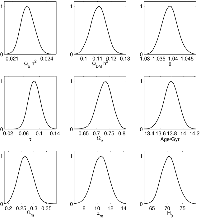
Figure 1: 1D marginalized posterior distribution of the background cosmological parameters (both input and derived) obtained by PPL fitting to WMAP7 data. Y-axis gives the probability from 0 to 1.

Figure 2 gives the 1D marginalized posterior distribution of the PPL inflationary parameters. The marginalized probability for $\nu_{s}$ peaks at $-0.04$ (corresponding to $n_{s}=0.96$ at the pivot point), and the marginalized probability for $\nu_{st}$ is found to be maximum at 0.0027. The $95\%$ marginalised limit of $\nu_{st}$ is found to be in the range $-0.016<\nu_{st}<0.022$. The plot of joint 2D marginalized posterior distribution of $\nu_{s}$ and $\nu_{st}$ is given by Figure 3. The colour of the figure shows how many times the CosmoMC has probed a specific area of the parameter space and the inner and outer closed contour lines indicate the 1 and 2-$\sigma$ likelihood contours.

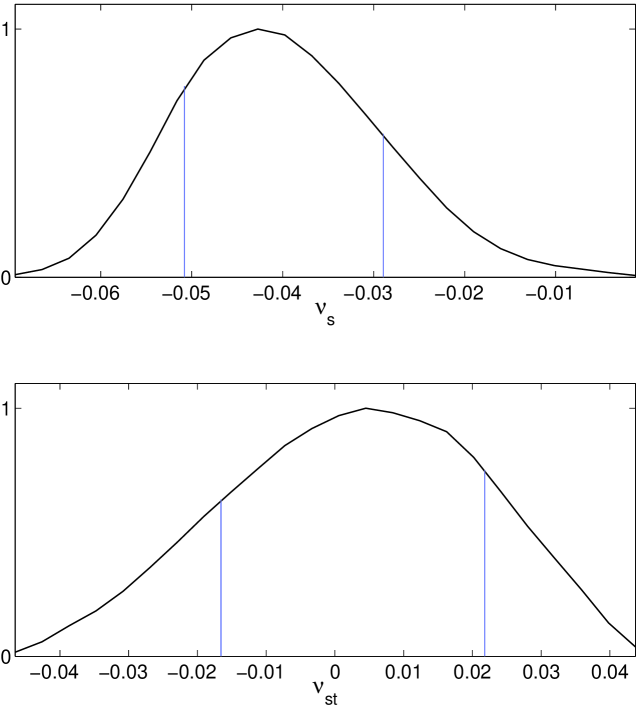
Figure 2: 1D marginalized posterior distribution of the PPL inflationary parameters $\nu_{s}$ and $\nu_{st}$ obtained by fitting to WMAP7 data. The $95\%$ marginalised limit on the parameters are shown by the vertical lines.

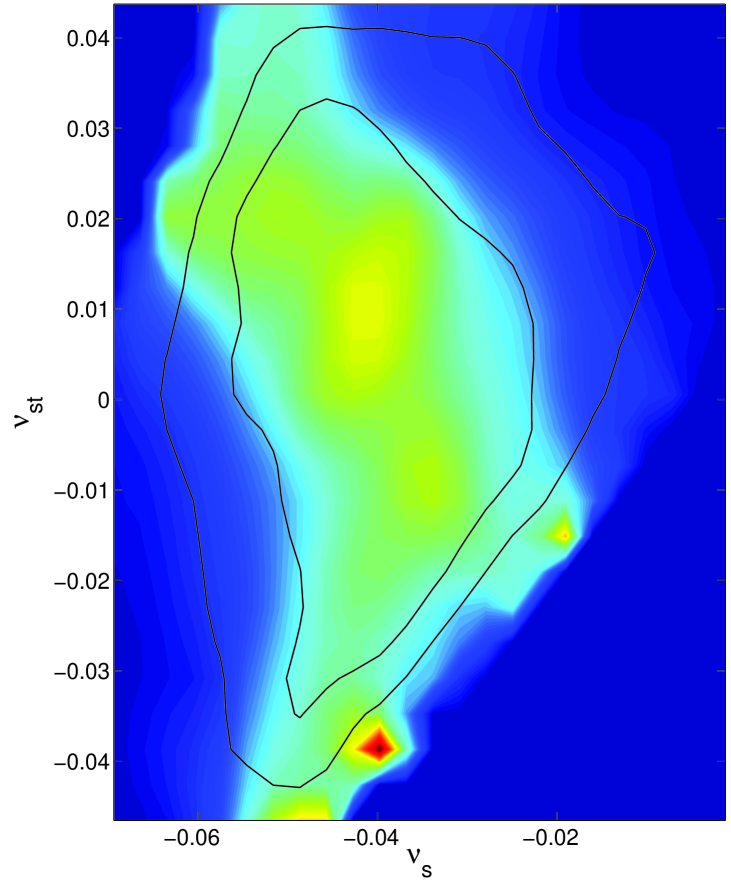
Figure 3: The joint 2D marginalized posterior distribution of $\nu_{s}$ and $\nu_{st}$

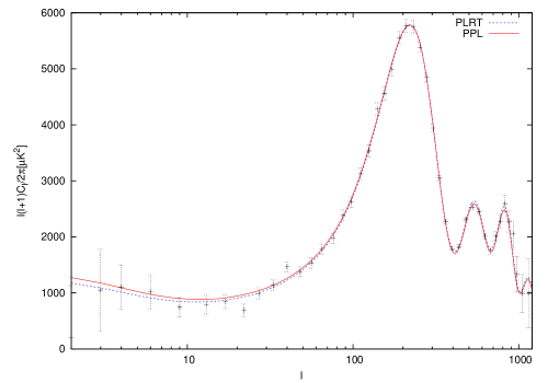
Figure 4: Best fit $C_{\ell}s$ for power-law (PLRT) (blue, dotted), power law with perturbative method (PPL)  (red, solid) and the WMAP7 binned data with related error bars

The best fit $C_{\ell}s$ for power law with running and tensor (PLRT) and power law with perturbative method (PPL) are presented in Figure 4. The WMAP7 binned data with related error bars are also plotted for comparison. It is clear that the PPL spectrum gives a very good fit to the observed data.

4 Conclusions and discussion

The high quality CMB data that has become available over the past few years and other observational data are just approaching the level of accuracy necessary to detect deviations from exact scale invariance and to distinguish between different inflationary models. The data indicates that the departure of the spectral index from exact scale invariance is likely to be small, $|n_{s}(k)-1|\ll 1$, which is in good agreement with predictions of the simplest inflationary scenarios. A perturbative procedure for studying inflation models with soft departures from scale free spectra is discussed in this paper. In [15] one of the authors forecast how well one can constrain $H(\phi)$ using WMAP and Planck data. The expected 1-$\sigma$ error ellipses [15] in the $(\partial\ln H/\partial\phi)^{2}$ - $(\partial^{2}\ln H/\partial\phi^{2})$ plane for a fixed target power law model, are now obtained with actual WMAP data as given in Figure 3.

The perturbed power law spectrum is confronted with the 7-year WMAP data. The best fit values that we obtained for both the input and derived parameters matches very well with those quoted by the WMAP team for power law inflationary models. Also it is interesting to note that the $\chi_{\rm eff}^{2}$ value we obtained by fitting the PPL spectrum to the WMAP7 spectrum is very slightly better than that for a simple power law spectrum (with and without tensors). We find that the parameters of inflation can be well determined by this perturbative method. In case of the standard power law spectrum one has to consider the scalar and tensor spectral indices $n_{s}$, $n_{t}$ and the running of scalar spectral index $n_{run}$ as separate independent parameters. Here, in the case of PPL just the two parameters $\nu_{s}$ and $\nu_{st}$ will capture all these. In addition, PPL spectra takes care of the running of tensor spectral index also, which is not possible to be estimated by the standard PL spectra as it is too small. In conclusion, the perturbed power law model helps to determine how the general models of inflation are best studied as ‘departures from the power law model’. The probable values of the ‘deviation parameter’ $\nu_{st}$ is found to be consistent with zero (contained between $-0.04<\nu_{st}<0.04$). More precise data from Planck [22] would be able to measure the deviations from power law spectra quite accurately and our PPL approach would help to analyse and understand the results in a better way.

5 Acknowledgments

We acknowledge the use of high performance computing system at IUCAA. We thank Rita Sinha for contributions during the early stages of this project. We thank Moumita Aich for useful commments on our paper. MJ acknowledges the support from U.G.C. Major research project grant, F.No.34-30/2008(SR) and the Associateship of IUCAA. TS acknowledges support from Swarnajayanti Fellowship, DST, India.

References

References

-
[1]
D. N. Spergel, R. Bean, O. Doré et al., Astroph. J. Suppl.
170, 377 (2007) [arXiv:astro-ph/0603449].
E. Komatsu, J. Dunkley, M.R. Nolta et al., Astroph. J. Suppl. 180, 330 (2009) [arXiv:0803.0547].
D. Larson, J. Dunkley, G. Hinshaw et al., (2010), [arXiv:1001.4635] - [2] C. J. MacTavish, P. A. R. Ade, J. J. Bock et al., Astroph. J. 647, 799 (2006) [arXiv:astro-ph/0507503].
- [3] A. Benoit, P. Ade, A. Amblard et al., Astron. Astroph. 399, L25 (2003) [arXiv:astro-ph/0210306].
-
[4]
A. A. Starobinsky, Phys. Lett. B 91, 99 (1980);
A. D. Linde, Phys. Lett. B 108, 389 (1982);
A. Albrecht and P. J. Steinhardt, Phys. Rev. Lett. 48, 1220 (1982);
A. D. Linde, Phys. Lett. B 129, 177 (1983) -
[5]
V. F. Mukhanov and G. V. Chibisov, JETP Lett. 33, 532 (1981);
S. W. Hawking, Phys. Lett. B 115, 295 (1982);
A. A. Starobinsky, Phys. Lett. B 117, 175 (1982);
A. H. Guth and S.-Y. Pi, Phys. Rev. Lett. 49, 1110 (1982). - [6] J.R. Bond, 1994, Testing inflation with the cosmic background radiation, in: M. Sasaki, ed., Relativistic Cosmology, Proc. 8th Nishinomiya-Yukawa Memorial Symposium (Academic Press), and references therein. (arXiv:astro-ph/9406075).
- [7] F. Lucchin & S. Matarrese, Phys. Rev. D32, 1316 (1985).
- [8] M B Hoffman & M S Turner, Phys. Rev. D64, 023506 (2001).
- [9] A.R. Liddle and D. H. Lyth, Cosmological Inflation and Large-Scale Structure (Cambridge University Press, 2000).
- [10] A. A. Starobinsky, JETP Lett. 82, 169 (2005) [arXiv:astro-ph/0507193].
- [11] D. S. Salopek and J. R. Bond, Phys. Rev. D42, 3936 (1990).
- [12] J. E. Lidsey et al., Rev.Mod.Phys., 69 373 (1997) and references therein. (arXiv:astro-ph/9508078).
- [13] W. H. Kinney, Phys. Rev. D56, 2002 (1997) [arXiv:hep-ph/9702427].
- [14] T. Souradeep, Ph.D. Thesis (1995).
- [15] T. Souradeep, J. R. Bond and L. Knox [arXiv:astro-ph/9802262].
- [16] D.H.Lyth and E.D.Stewart, Phys. Lett. B 274, 168 (1992).
- [17] E.D. Stewart and D.H. Lyth, Phys. Lett. B 302, 171 (1993) [arXiv:gr-qc/9302019].
-
[18]
http://cosmologist.info/cosmomc/
A. Lewis and S. Bridle, Phys. Rev. D66, 103511 (2002). - [19] A. Lewis, A. Challinor and A. Labensky, Astrophysics J. 538 473 (2002).
- [20] http://lambda.gsfc.nasa.gov/
- [21] E. Komatsu, K. M. Smith, J. Dunkley et al., arXiv:1001.4538 (2010).
- [22] www.esa.int/planck