Abstract

This paper presents a graphical method for comparing performance of Markov Chain Monte Carlo methods. Most researchers present comparisons of MCMC methods using tables of figures of merit; this paper presents a graphical alternative. It first discusses the computation of autocorrelation time, then uses this to construct a figure of merit, log density function evaluations per independent observation. Then, it demonstrates how one can plot this figure of merit against a tuning parameter in a grid of plots where columns represent sampling methods and rows represent distributions. This type of visualization makes it possible to convey a greater depth of information without overwhelming the user with numbers, allowing researchers to put their contributions into a broader context than is possible with a textual presentation.

1 Introduction

Markov Chain Monte Carlo is a class of computational methods with which a user simulates a Markov chain whose stationary distribution is a target distribution of interest, generating a dependent sample from the target distribution. When choosing between MCMC methods, a user must trade off their own effort, computation time, and accuracy of results.

While many methods are documented in the literature, end-users gravitate to two classic methods: Gibbs sampling (when the full conditional distributions can be sampled from) and Metropolis–Hastings updates with Gaussian proposals (when they cannot). These are widely available and well understood, but often inefficient. Perhaps, if better comparisons of MCMC methods were possible, a consensus would emerge on which widely applicable modern methods perform best.

In the computational statistics literature, most researchers compare the computational efficiency of methods with tables of autocorrelation times, effective sample sizes, or other similar measures. For example, in the Journal of Computational and Graphical Statistics Vol. 19 No. 2, four papers presented comparisons of MCMC methods; all four compared their proposed methods this way (Giordani and Kohn,, 2010; Liechty and Lu,, 2010; Niemi and West,, 2010; Papastamoulis and Iliopoulos,, 2010).

By using tabular comparisons, researchers limit themselves to presenting only a few data points. This is compelling when the target distribution is important in its own right, the set of reasonable samplers is small, and none of the samplers require tuning. However, if a researcher wants to present a method for general use, readers will find a broader comparison useful. This paper presents a graphical alternative to tables that allows researchers to compare their MCMC methods to existing ones without overwhelming readers with numbers.

To quantify the efficiency of a simulation, I will use the autocorrelation time—also called correlation length—the number of observations from an MCMC simulation equivalent to a single independent observation. If an MCMC simulation has an autocorrelation time of $\tau$, estimates based on this simulation will have standard errors approximately the same as those of an independent sample a factor of $\tau$ smaller. Section 2 will discuss autocorrelation time in detail.

Section 3 describes a collection of four distributions and four MCMC methods. Using these distributions and methods, section 4 shows that measuring a method’s speed with either processor usage or log-density function evaluations will often lead to the same conclusions.

Section 5 presents the main contribution of this paper: a method for comparing MCMC methods by plotting log density evaluations per iteration times autocorrelation time against a tuning parameter in a grid of plots where rows represent distributions and columns represent methods. This is supported with an example using the distributions and methods described in section 3.

Section 6 develops this idea further, showing that any three dimensions of the comparison scenario may be examined simultaneously. This is demonstrated with an example that shows how a single method’s performance varies as a function of problem dimension and two tuning parameters.

2 Autocorrelation time

Suppose the goal in running an MCMC simulation is to estimate the expectation of a random variable $X$ that is some function of the Markov chain state. Based on a sample $(X_{1},\ldots,X_{n})$, we can estimate $E(X)$ with:

$$\hat{\mu}_{n}=\frac{X_{1}+\cdots+X_{n}}{n}$$ (1)

Assuming $X$ has finite variance, define the autocorrelation function (ACF) at lag $k$ as:

$$\rho_{k}=\frac{\operatorname*{cov}(X_{i},X_{i+k})}{\operatorname*{var}(X_{i})}$$ (2)

Assume the chain has reached its stationary distribution, so $\rho_{k}$ does not depend on $i$. The autocorrelation time is then (Straatsma et al.,, 1986, p. 91):

$$\tau=1+2\sum_{k=1}^{\infty}\rho_{k}$$ (3)

If this sum converges—which it will for all geometrically ergodic Markov chains (Mira,, 1998)—then:

$$\frac{n}{\tau}\operatorname*{var}(\hat{\mu}_{n})\rightarrow\operatorname*{var}(X_{i})$$ (4)

When the states are independent, the autocorrelations are zero, so according to equation 3, $\tau$ is one, and equation 4 becomes the usual formula for the variance of a sample mean.

2.1 Estimating the autocorrelation time

One cannot estimate the autocorrelation time by plugging sample autocorrelations into equation 3. The usual formula for the sample ACF (based on equation 2) is:

$$\hat{\rho}_{k}=\frac{1}{ns_{X}^{2}}\sum_{i=1}^{n-k}(X_{i}-\hat{\mu}_{n})(X_{i+k}-\hat{\mu}_{n})$$ (5)

where $s_{X}^{2}$ is the sample variance of $(X_{1},\ldots,X_{n})$. The sample ACF is not defined for lags greater than $n-1$, and $\hat{\rho}_{1}+\cdots+\hat{\rho}_{n-1}$, the sum of the first $n-1$ terms of equation 3, has a variance that does not converge to zero as the sample size goes to infinity, so an estimator of $\tau$ based on this sum would not be consistent.

Instead, taking the approach of CODA’s spectrum0.ar and effectiveSize functions (Plummer et al.,, 2006), we model the Markov chain as an AR($p$) process, where $p$ is chosen with AIC. Because the ACF of an AR($p$) process is a function of its model parameters, we can avoid explicitly computing the ACF for large lags. Suppose we have an AR($p$) model of the form:

$$X_{t}=\mu+\pi_{1}X_{t-1}+\cdots+\pi_{p}X_{t-p}+a_{t},\qquad a_{t}\sim N(0,\sigma_{a}^{2})$$ (6)

Let ${\bm{\pi}}$ denote the vector $(\pi_{1},\ldots,\pi_{p})^{T}$. Let ${\bm{\rho}}$ denote the vector $(\rho_{1},\ldots,\rho_{p})^{T}$, with $\hat{\bm{\rho}}$ denoting its sample estimate from equation 5. The true mean, $\mu$, is often known for test distributions; if it is not, we can estimate it with $\hat{\mu}_{n}$. We use these estimates to compute an estimate of ${\bm{\pi}}$, denoted by $\hat{\bm{\pi}}$, and the asymptotic covariance matrix of $\hat{\bm{\pi}}$, denoted by ${\bm{V}}$, with the Yule–Walker method (Wei,, 2006, pp. 136–138).

Denote a vector of $p$ ones by ${\bm{1}}_{p}$. The autocorrelation time of the process defined by equation 6 is:

$$\tau=\frac{1-{\bm{\rho}}^{T}{\bm{\pi}}}{\left(1-{\bm{1}}_{p}^{T}{\bm{\pi}}\right)^{2}}$$ (7)

By substituting $\hat{\bm{\rho}}$ for ${\bm{\rho}}$ and $\hat{\bm{\pi}}$ for ${\bm{\pi}}$ in equation 7, we obtain an estimate of the autocorrelation time:

$$\hat{\tau}=\frac{1-\hat{\bm{\rho}}^{T}\hat{\bm{\pi}}}{\left(1-{\bm{1}}_{p}^{T}\hat{\bm{\pi}}\right)^{2}}$$ (8)

Equation 7 is based on the observation of Heidelberger and Welch, (1981) that the autocorrelation time and the spectrum of a time series at frequency zero are identical. The spectrum of an autoregressive process is defined by equation 12.2.8b of Wei, (2006, pp. 274–275). I use equation 7.1.5 of Wei, (2006, p. 137) to remove the dependence of Wei’s equation 12.2.8b on the innovation variance, $\sigma_{a}^{2}$. For more information on modeling simulations with AR processes, see Fishman, (1978, §5.10).

2.2 Confidence intervals

A measure of the uncertainty in the estimated autocorrelation time is often useful. Here, I describe one method for generating confidence intervals for $\tau$ using ${\bm{V}}$, the asymptotic covariance matrix of $\hat{\bm{\pi}}$.

The sample ACF to lag $p$ is a function of $\hat{\bm{\pi}}$, so equation 8 does not depend monotonically on $\hat{\bm{\pi}}$ as one might think, making deriving an expression for a closed-form confidence interval for $\tau$ difficult. Instead, one can simulate a set $({\bm{\pi}}^{(1)},\ldots,{\bm{\pi}}^{(m)})$ with elements that are each multivariate Gaussian with mean $\hat{\bm{\pi}}$ and covariance ${\bm{V}}$. Each ${\bm{\pi}}^{(k)}$ can be used to generate a corresponding ${\bm{\rho}}^{(k)}$ (Wei,, 2006, p. 47, equation 3.1.28) as done in the R function ARMAacf. These ${\bm{\pi}}^{(k)}$ and ${\bm{\rho}}^{(k)}$ can be substituted into equation 8 to generate estimates of $\tau$. The quantiles of these simulated estimates can then be used to generate a confidence interval.

However, not all the simulated ${\bm{\pi}}^{(i)}$ will define stationary processes because the true sampling distribution of $\hat{\bm{\pi}}$ is not multivariate normal. If the equation:

$$1=\pi^{(i)}_{1}z+\cdots+\pi^{(i)}_{p}z^{p}$$ (9)

has roots inside the unit circle, the resulting AR($p$) process is not stationary (Wei,, 2006, p. 26). In this case, equation 7 does not apply, and the estimate $\hat{\tau}=\infty$ should be used instead. If more than 2.5% of the simulated ${\bm{\pi}}^{(i)}$ define nonstationary AR processes, a 95% confidence interval will be unbounded; this can be seen in several grid cells of figure 2.

2.3 Alternatives

Equation 7 is not the only way to estimate the autocorrelation time. One can estimate it with the sample autocorrelation function evaluated out to some moderate lag chosen by some rule such as the initial convex sequence (Geyer,, 1992). This method and equation 7 tend to produce similar estimates. One advantage of equation 7 is the relative ease with which confidence intervals may be computed. A second alternative is to fit a polynomial model to the log-spectrum of the sample autocorrelation function (Heidelberger and Welch,, 1981). This method can generate confidence intervals, but has two free parameters and is difficult to apply to highly correlated chains (Plummer et al.,, 2010). For more information on the estimation of autocorrelation times, see Thompson, (2010).

2.4 Multivariate distributions

Quite often, some coordinates mix faster than others. Consider the linear combination of two coordinates:

$$Y=aX^{(1)}+bX^{(2)}$$ (10)

If the two coordinates have autocorrelation times $\tau^{(1)}$ and $\tau^{(2)}$, the variance of the mean of $Y$ will be:

$$\operatorname*{var}(\bar{Y}_{n}) =a^{2}\operatorname*{var}(\bar{X}_{n}^{(1)})+2ab\operatorname*{cov}(\bar{X}_{n}^{(1)},\bar{X}_{n}^{(2)})+b^{2}\operatorname*{var}(\bar{X}_{n}^{(2)})$$ (11)

$$=a^{2}\operatorname*{var}(\bar{X}^{(1)})+2ab\sqrt{\operatorname*{var}(\bar{X}^{(1)})\operatorname*{var}(\bar{X}^{(2)})}\operatorname*{corr}(\bar{X}_{n}^{(1)},\bar{X}_{n}^{(2)})+b^{2}\operatorname*{var}(\bar{X}^{(2)})$$

$$\approx a^{2}\frac{\tau^{(1)}}{n}\operatorname*{var}(X^{(1)})+2ab\frac{\sqrt{\tau^{(1)}\tau^{(2)}}}{n}\sqrt{\operatorname*{var}(X^{(1)})\operatorname*{var}(X^{(2)})}\operatorname*{corr}(\bar{X}_{n}^{(1)},\bar{X}_{n}^{(2)})+b^{2}\frac{\tau^{(2)}}{n}\operatorname*{var}(X^{(2)})$$

Because the correlation between the two coordinate means is bounded to $[-1,1]$, if the coordinates have substantially different autocorrelation times, the first or last term will dominate this variance. So, the autocorrelation time of any linear combination of coordinates will be approximately the autocorrelation time of the slowest-mixing component. All comparisons of MCMC methods on multivariate distributions in this paper take this approach, reporting figures of merit based on the slowest-mixing component.

The argument of this section only addresses linear combinations of components. Nonlinear functions of multiple components—or even a single component—may have substantially different autocorrelation times than the autocorrelation times of any linear combination of components. The mixing rates of all possible functions cannot be summarized in a single number; additional information about which functions are relevant would be necessary.

3 Methods and distributions for demonstration

Sections 4 and 5 both compare four MCMC methods on four distributions. Since this paper is intended to demonstrate methods of comparison rather than advocate a particular MCMC sampler, I attempted to choose a representative collection of samplers and distributions.

3.1 MCMC methods

Each MCMC method compared has a single tuning parameter. The methods are:

• Adaptive Metropolis: the adaptive Metropolis–Hastings algorithm described by Roberts and Rosenthal, (2009, sec. 2). The tuning parameter is the standard deviation of the non-adaptive component of the proposal distribution, which they fixed at 0.1 (in their equation 2.1). This version of Metropolis uses multivariate Gaussian proposals with a covariance matrix determined by previous states. Unlike the version of Roberts and Rosenthal,, the implementation used here stops adapting after the burn-in period.

• Univariate Metropolis: Metropolis with transitions that update each coordinate sequentially. The proposals are Gaussian with standard deviation equal to the tuning parameter.

• Shrinking Rank: the shrinking-rank slice sampler described by Thompson and Neal, (2010, sec. 5). The tuning parameter is $\sigma_{c}$, the initial crumb standard deviation.

• Step-out Slice: slice sampling with stepping out, updating each coordinate sequentially, as described by Neal, (2003, sec. 4). The tuning parameter is $w$, the initial estimate of slice size.

3.2 Distributions

The distributions compared are:

• $\operatorname{Gamma}(2,1)$: A one dimensional Gamma distribution with density proportional to $xe^{-x}$.

• $N_{4}(\rho=0.999)$: A four dimensional Gaussian centered at $(1,2,3,4)$ with covariance matrix:

  $${\bm{\Sigma}}=\begin{bmatrix}1&0.999&0.999&0.999\\ 0.999&1&0.999&0.999\\ 0.999&0.999&1&0.999\\ 0.999&0.999&0.999&1\end{bmatrix}$$ (12)

  This has a condition number of 2870.

• Eight Schools: A multilevel model in ten dimensions, consisting of eight group means and hyperparameters for their mean and log-variance (Gelman et al.,, 2004, pp. 138–145). Its covariance is well-conditioned.

• Mixture Ten: A ten-component Gaussian mixture in $\mathbb{R}^{10}$. Each mode is a spherically symmetric Gaussian with unit variance. The modes were drawn from a uniform distribution on a hypercube with edge-length ten.

4 Processor usage and log density evaluations

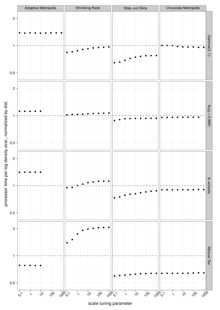
Figure 1: The ratio of processor usage to log density evaluations, normalized by distribution. One can see that this ratio does not depend much on method choice or tuning parameter; see section 4 for discussion. Each simulation is of length 50,000. The gaps in some of the Adaptive Metropolis plots correspond to simulations where the autocorrelation time could not be estimated.

Before comparing performance of methods on a distribution, we must choose a figure of merit. Here, I use the distributions and methods of section 3 to justify the choice of log-density evaluations per MCMC iteration multiplied by autocorrelation time.

If a user’s goal is to estimate a parameter to a specific accuracy, they would want to choose an MCMC method that minimizes processor time per iteration multiplied by autocorrelation time. But, using processor usage on a researcher’s machine is problematic because it depends on irrelevant factors such as the type of machine the researcher is using, other simultaneous tasks running on the machine, etc. Even identically configured simulations may generate different results.

An alternative to measuring processor usage is counting log-density function evaluations. Initialized with the same random seed, an MCMC simulation that does not use information about the target distribution other than its log-density function would evaluate this function the same number of times on machines of different speeds, on the same machine with different concurrent processes, and often even when implemented in different programming languages. However, this measure does not capture the overhead of the MCMC method, nor does it capture different ways a distribution can be represented to the method. For example, some methods require gradients to be computed, increasing the processor time per evaluation. Other methods, like those based on Gibbs sampling, may not compute log densities at all.

To see the comparability of these two measures, at least on the distributions and methods described in section 3, see figure 1, which plots the ratio of processor usage to log-density function evaluations for those samplers and distributions for a range of tuning parameters. The ratios are normalized to the median processor time for a function evaluation over the simulations of that distribution. If processor usage and log density evaluations were perfectly comparable, every plotted point would lie on the dashed horizontal line indicating a ratio of one. For the simulations in figure 1, the measures are at most a small multiple off from each other.

A minor anomaly occurs with the Mixture Ten distribution when simulated with Shrinking Rank. Shrinking Rank is the only method that computes gradients, and the Mixture Ten distribution has gradient evaluation code that is unusually inefficient relative to its log density evaluation code. The ratio does not exceed two, though, while MCMC method efficiency differences are often several powers of ten. Because no significant differences in ratios are observed, I am inclined to believe that comparing processor usage and comparing log density evaluations will yield similar conclusions regarding the merits of various MCMC methods.

5 Demonstration results

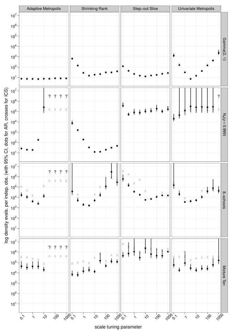
Figure 2: A demonstration of graphical comparison of performance of MCMC samplers. Columns of plots represent samplers; rows represent distributions. Each simulation is of length 50,000. At a glance, a researcher can see how 144 simulations relate to each other. See section 5 for discussion.

The figures of merit described in sections 2 and 4 provide a way of quantifying the performance of the MCMC methods described in section 3.1 on the distributions described in section 3.2. I simulated each of these distributions with each sampler for nine values of the sampler’s tuning parameter in the range $0.1$ to $1000$. Each chain had a length of 50,000. Treating the first fifth of each chain as a burn-in period, I computed the autocorrelation time of each simulation using the method of section 2 and multiplied it by the average number of log density evaluations the simulation needed per iteration to generate an estimate of the number of log density evaluations per independent observation. Smaller values indicate better performance.

In figure 2, I compare the evaluations per independent observation by plotting them as dots with a 95% simulation-based confidence interval against the tuning parameter for each combination of distribution and method. Question marks indicate simulations with too few unique states to identify an AR model.

The superimposed crosses represent the same figure of merit computed with the initial convex sequence (Geyer,, 1992) instead of the AR model described in section 2.1. The two estimators mainly differ when the estimated autocorrelation time is close to or greater than the simulation length, as is the case for the Mixture Ten simulations. In this case, they agree inasmuch as both estimators indicate that the simulation is too short. Another discrepancy occurs with Step-out Slice on Eight Schools with tuning parameters in the range $[0.3,10]$. These simulations are notable for occasionally getting stuck briefly in a single part of the state space.

5.1 Between-cell comparisons

Scanning an individual cell in the grid of plots, one can see how performance varies with the tuning parameter. Scanning down columns of the grid of plots, one can see how performance varies from distribution to distribution for a given MCMC method. Scanning across rows of the grid of plots, one can see how performance varies from method to method for a given distribution.

Doing this, several patterns emerge. For example, one can see that Adaptive Metropolis performs consistently well for a variety of tuning parameters, as long as the tuning parameter is smaller than the square root of the smallest eigenvalue of the distribution’s covariance. Either it performs well, or does not converge at all. This suggests that Adaptive Metropolis users uncertain about the distribution they are sampling from should err in the direction of small tuning parameters.

A second pattern is that Univariate Metropolis tends to have U-shaped comparison plots. Tuning parameters that are either too small or too large lead to unacceptable performance. And, the lowest points on these plots are still above the flat parts of the Adaptive Metropolis plots. On low-dimensional distributions like these, where the sampler does not know the structure of the target density, Adaptive Metropolis can be considered to dominate Univariate Metropolis.

Reading across columns, one can see different sorts of patterns. For example, the Gamma(2,1) distribution has a relatively flat sequence of figures of merit across the row of grid cells, suggesting that sampling from this distribution is not sensitive to choice of method (if Univariate Metropolis is excluded) or tuning parameter. The $N_{4}(\rho=0.999)$ row is also flat within cells, but not between them, suggesting that for that distribution, one needs to pay attention to the choice of method, but not as much to the tuning parameter.

5.2 Within-cell comparisons

A different sort of pattern can be seen in slopes of the lines traced out by the plot symbols. For Univariate Metropolis and the shrinking rank method on Gamma(2,1) and Shrinking Rank on $N_{4}(\rho=0.999)$, for tuning parameters less than one, an increase in the tuning parameter by a factor of ten leads to a factor of almost one hundred improved performance—a slope of $-2$ in the log domain. For these tuning parameters the Markov chains are nearly a one-dimensional random walk; such a random walk will travel some distance in a number of steps proportional to the square of the distance (Feller,, 1968, p. 90).

This can be contrasted with the slope of the plot symbols for Step-out Slice, which is close to $-1$ for small tuning parameters on the Gamma(2,1) and Eight Schools distributions. This sampler requires a number of log density function evaluations linear in the ratio of slice width to tuning parameter to compute a slice estimate, so increasing the tuning parameter by some factor improves the performance by that factor.

A pattern in the slopes for large parameters can be seen with Univariate Metropolis on Gamma(2,1) with tuning parameters larger than one. In those simulations, multiplying the tuning parameter by ten degrades performance by a factor of approximately ten—a slope of one in the log domain. Increasing the tuning parameter by some factor reduces the acceptance rate by approximately that factor when the tuning parameter is large.

This behavior contrasts with the two slice samplers, whose figures of merit follow logarithmic curves for large tuning parameters on Gamma(2,1). Each rejected proposal reduces the estimated slice size by, on average, a factor of two, so an increase in a tuning parameter above the optimal value by some factor increases the computation cost by the log of that factor.

None of the patterns of this section would be easily visible if the results were presented in tabular form. Figure 2 shows summaries of 144 simulations, more than could be absorbed by a reader if presented as text.

6 A second demonstration

Figure 3: A demonstration of graphical comparison of performance of a single sampler, Adaptive Metropolis, with two tuning parameters. Columns of plots represent different values of one tuning parameter, $\beta$; the other is plotted on the horizontal axis of the subplots. Rows of plots correspond to increasing dimensions of badly-scaled Gaussian distributions. Each simulation is of length 40,000. See section 6 for discussion.

While plots like figure 2 allow a broad comparison of distributions and methods, it is often necessary to drill down further. The same type of plot can be used when varying extra parameters associated with either the distribution or the MCMC method. Figure 3 is an example of such a comparison. It focuses just on Adaptive Metropolis sampling from badly-scaled Gaussians.

One tuning parameter to Adaptive Metropolis is $\beta$, the fraction of proposals drawn from a spherical Gaussian instead of a Gaussian with a learned covariance. Roberts and Rosenthal, (2009) suggest the value of 0.05. In this example, I vary it from $0.001$ to $0.95$.

I simultaneously consider the effect of dimensionality on the performance of the method. Each target distribution is a multivariate Gaussian with uncorrelated parameters with variance equal to 1000 in the first coordinate and one in the rest. The problem dimension ranges from 2 to 128.

As with the simulations of figure 2, Adaptive Metropolis performs well when the principal tuning parameter is smaller than the square root of the smallest eigenvalue of the target distribution’s covariance, in this case one. While the method performs better in low dimensional spaces, this performance does not vary much with $\beta$ in any of the dimensions simulated.

7 Discussion

Section 5 shows the variation in performance of MCMC methods while varying method, distribution, and one tuning parameter. Section 6 shows the variation in performance of a single MCMC method while varying two tuning parameters and one distribution parameter. In general, one may use the plots described in this paper to compare performance of MCMC methods while varying any three factors. Comparing performance with tabulated summary statistics, in contrast, only allows researchers to study variation in one factor at once, a significant disadvantage.

One might wonder, then, how one could visualize performance as more than three factors vary simultaneously. While it may be useful, computational limits become an obstacle as the number of parameters increases. Figure 2 compares 144 simulations. Even if there were a clear way to visualize variation in four or five factors, one would need to run thousands of simulations to make such a plot. The plots of this paper display approximately as much information as is currently feasible to gather.

Other variations on these plots are possible. The most common is to replace confidence intervals by multiple plot symbols, each representing a replication of the same simulation with a different random seed, so that multiple symbols are plotted in a column for a given tuning parameter. In this case, making the symbols partially transparent makes the graph easier to read.

If one is willing to forego all measures of uncertainty under replication, one can omit the confidence intervals and plot figures of merit for multiple values of a second factor, such as a second tuning parameter, in a single grid cell, differentiating levels of this factor by color or plot symbol. However, this technique can produce confusing graphs if the factor represented by color or plot symbol is not naturally nested in the factor represented by columns of plots, so one should not vary a factor like problem dimension inside a single grid cell.

8 Software

SamplerCompare is an R package that allows researchers to run simulations and generate plots like those described in this paper. It supports MCMC methods and distributions implemented in R and C and is available on CRAN at http://cran.r-project.org/web/packages/SamplerCompare.

9 Acknowledgments

I would like to thank Radford M. Neal for his extensive comments on the draft manuscript.

References

- Feller, (1968) Feller, W. (1968). An Introduction to Probability Theory and its Applications, Volume I, Third Edition. John Wiley and Sons.
- Fishman, (1978) Fishman, G. S. (1978). Principles of Discrete Event Simulation. John Wiley and Sons.
- Gelman et al., (2004) Gelman, A., Carlin, J. B., Stern, H. S., and Rubin, D. B. (2004). Bayesian Data Analysis, Second Edition. Chapman and Hall/CRC.
- Geyer, (1992) Geyer, C. J. (1992). Practical Markov Chain Monte Carlo. Statistical Science, 7(4):473–511.
- Giordani and Kohn, (2010) Giordani, P. and Kohn, R. (2010). Adaptive independent Metropolis–-Hastings by fast estimation of mixtures of normals. Journal of Computational and Graphical Statistics, 19(2):243–259.
- Heidelberger and Welch, (1981) Heidelberger, P. and Welch, P. D. (1981). A spectral method for confidence interval generation and run length control in simulations. Communications of the ACM, 24(4):233–245.
- Liechty and Lu, (2010) Liechty, M. W. and Lu, J. (2010). Multivariate normal slice sampling. Journal of Computational and Graphical Statistics, 19(2):281–294.
- Mira, (1998) Mira, A. (1998). Ordering, Slicing, and Splitting Monte Carlo Markov Chains. PhD thesis, University of Minnesota.
- Neal, (2003) Neal, R. M. (2003). Slice sampling. Annals of Statistics, 31:705–767.
- Niemi and West, (2010) Niemi, J. and West, M. (2010). Adaptive mixture modeling Metropolis methods for Bayesian analysis of nonlinear state-space models. Journal of Computational and Graphical Statistics, 19(2):260–280.
- Papastamoulis and Iliopoulos, (2010) Papastamoulis, P. and Iliopoulos, G. (2010). An artificial allocations based solution to the label switching problem in Bayesian analysis of mixtures of distributions. Journal of Computational and Graphical Statistics, 19(2):313–331.
- Plummer et al., (2006) Plummer, M., Best, N., Cowles, K., and Vines, K. (2006). CODA: Convergence diagnosis and output analysis for MCMC. R News, 6(1):7–11.
- Plummer et al., (2010) Plummer, M., Best, N., Cowles, K., and Vines, K. (2010). CODA Reference Manual.
- Roberts and Rosenthal, (2009) Roberts, G. O. and Rosenthal, J. S. (2009). Examples of adaptive MCMC. Journal of Computational and Graphical Statistics, 18(2):349–367.
- Straatsma et al., (1986) Straatsma, T. P., Berendsen, H. J. C., and Stam, A. J. (1986). Estimation of statistical errors in molecular simulation calculations. Molecular Physics, 57(1):89–95.
- Thompson, (2010) Thompson, M. B. (2010). A comparison of methods for computing autocorrelation time. Technical Report 1007, Dept. of Statistics, University of Toronto. arXiv:1011.0175v1 [stat.CO].
- Thompson and Neal, (2010) Thompson, M. B. and Neal, R. M. (2010). Covariance-adaptive slice sampling. Technical Report 1002, Dept. of Statistics, University of Toronto. arXiv:1003.3201v1 [stat.CO].
- Wei, (2006) Wei, W. W. S. (2006). Time Series Analysis: Univariate and Multivariate Methods, Second Edition. Pearson/Addison Wesley.