DISCRETE MULTISCALE ANALYSIS:
A BIATOMIC LATTICE SYSTEM

Abstract

We discuss a discrete approach to the multiscale reductive perturbative method and apply it to a biatomic chain with a nonlinear interaction between the atoms. This system is important to describe the time evolution of localized solitonic excitations.

We require that also the reduced equation be discrete. To do so coherently we need to discretize the time variable to be able to get asymptotic discrete waves and carry out a discrete multiscale expansion around them. Our resulting nonlinear equation will be a kind of discrete Nonlinear Schrödinger equation. If we make its continuum limit, we obtain the standard Nonlinear Schrödinger differential equation.

1 INTRODUCTION

Nonlinear systems, and in particular nonlinear discrete systems, are gaining an increasing impact in modern science [33].

In 1955 Fermi, Pasta and Ulam (FPU) [14] considered a unidimensional chain of atoms with nonlinear nearest neighbouring interaction to verify if nonlinearity could produce energy equipartition. Instead, they found recurrence, i.e. the motion of the chain for small energies was almost periodic [43]. To explain this result Kruskal and Zabusky found in 1965 [42] a connection between the FPU system and the Korteweg–De Vries equation (KdV), an equation introduced in fluid dynamics to describe one dimensional surface waves in the shallow water context [20]. By introducing the Inverse Scattering Transform, they where able to solve the Cauchy problem for the KdV equation [15] and to prove the existence of soliton solutions.

In 1967 Toda [37] considered a dynamical system with exponential interaction, $U(r)=e^{-r}+r-1$, the ”Toda potential”, whose small amplitude approximation gives the FPU system, and shares many of the integrability properties of the KdV equation. So the FPU system turns out to be an approximation of a discrete soliton model.

Later more complicate atomic chains have been considered, as, for example, the biatomic one [6, 16, 11, 12, 26, 9]. These systems have various applications in physics and biology as, for example, in the study of ferroelectric perovskites, materials that, in certain crystallographic directions have an almost unidimensional frame, and in organic molecular chains. A biatomic chain of neighboring atoms $A_{1}$ and $A_{2}$ is described by the discrete independent variable $n$ and a continuous time $t$. However, the simplest nonlinear coupled lattice dynamical equations one can construct for this system are not solvable. Only special exact solutions may be found.

Multiscale expansions [20, 7, 8, 19, 21, 35, 36] have proved to be important tools to find approximate solutions for many physical problems by reducing a given nonlinear partial differential equation to a simpler equation, which is often integrable [5]. Recently, few attempts to carry over this approach to partial difference equations have been proposed [2, 22, 23, 10, 32]. Almost all approaches considered contain some approximation, either based on physical or on mathematical reasoning as scaling transformations of the lattice provide a nonlocal result. In the following we prefer to stick to mathematical approximations as in this case it will be more evident what to do to improve the final result [17].

In ref [9] a biatomic chain obtained as a first nonlinear approximation of a complex Lenard–Jones interaction between atoms has been considered. There the multiscale expansion of the continuous limit of the lattice model showed that the modulation of periodic solutions is governed by the Nonlinear Schrödinger differential Equation (NLSE). Here we consider the same model but we are interested in carrying out the multiscale expansion on the lattice, i.e. we are looking for a lattice equation which in the asymptotic regime approximate the biatomic nonlinear lattice. To do so we need to discretize time to be able to allow for discrete asymptotic waves. If we keep a continuous time variable an asymptotic wave travelling on the lattice by necessity will be described by a continuous variable. So by necessity we go over to a differential system.

Discretization of variables, besides representing an interesting problem in mathematical physics for its computerizability, it is also useful in itself. Measurements, for example, are based on sampling of physical variables such as space and time. It follows that physical models in which variables are defined on the lattice are easier to be compared with the real world we see in our measurements.

In this work, we propose to continue the previous researches of biatomic chains considering both $t$ and $n$ as discrete variables. In particular, we shall assume, as these authors, that the system has a unharmonic cubic potential as in nature, potentials usually are non–symmetric. We shall thus apply a discrete multiscale reductive perturbative method to the model introduced by Campa et. al.[9] consisting of a biatomic chain with a nonlinear nearest neighbour interaction.

In Section 2 we describe in detail the biatomic chain and write down the dynamical equations. Then in Section 3 we introduce some notions of discrete calculus and multiple scales defined on the lattice which we apply in Section 4 to the biatomic chain introduced in Section 2. In Section 5 we analyze the resulting nonlinear discrete equation obtained and carry out its continuum limit. Finally, in Section 6 we draw some final conclusions.

2 THE MODEL

We want to describe here a chain suitable to represent, for example, an $\alpha$-helix channel, see Scott (1999) [33]. Our model consists of a biatomic chain formed by a sequence of pairs of neighboring atoms $A_{1}$ and $A_{2}$, with masses $M_{1}$ and $M_{2}$, respectively. Each pair, made of an atom of mass $M_{1}$ and the following one of mass $M_{2}$, can be considered as a ”molecule”. We denote by the index $n$ the $n^{th}$ molecule formed by the atom $A_{1}$ and $A_{2}$ (see Fig. 1).

Fig. 1: Pattern of a biatomic molecular chain in one dimension. The chain is formed by a sequence of pairs of neighboring atoms $A_{1}$ and $A_{2}$. The displacements of the atoms of the molecule $n$ are indicated with $x_{n}$ and $y_{n}$.

Let us indicate with $x_{n}(t)$ and $y_{n}(t)$ the displacements of the atoms $A_{1}$ and $A_{2}$ belonging to the same molecule $n$. For each atom, we assume only nearest neighbourg interactions. Then, the total potential of the chain is given by

$$U=\sum_{n}\{U_{1}(y_{n}-x_{n})+U_{2}(x_{n+1}-y_{n})\},$$ (1)

where $U_{1}$ is the intramolecular potential, between atoms belonging to the same molecule, and $U_{2}$ is the potential between different molecules.

Given a natural [6, 3, 38] asymmetric potential with an absolute minimum in the equilibrium position as, for example, a Lenard–Jones potential, by taking the first terms of its Taylor expansion around the equilibrium position we can write the potentials $U_{1}$ and $U_{2}$ as

$$U_{1}(r)=\frac{1}{2}k_{1}r^{2}+\frac{\epsilon}{3}\beta_{1}r^{3},\qquad U_{2}(r)=\frac{1}{2}k_{2}r^{2}+\frac{\epsilon}{3}\beta_{2}r^{3},$$

where $k_{1}$ and $k_{2}$ are the harmonic constants, $\beta_{1}$ and $\beta_{2}$ are the cubic interaction constants and $\epsilon$ is a small parameter which will play the role of the perturbative parameter. We assume that the interaction between atoms of the same site is stronger than that of atoms of different sites; thus $k_{1}$$>$${k_{2}}$ and $|\beta_{1}|$$>$$|\beta_{2}|$. So, the Hamiltonian of our molecular chain turns out to be

$$\begin{array}[]{c}H=\sum_{n}\{\frac{1}{2}[M_{1}\dot{x}_{n}^{2}+M_{2}\dot{y}_{n}^{2}]+\frac{1}{2}[k_{1}(y_{n}-x_{n})^{2}+k_{2}(x_{n+1}-y_{n})^{2}]\\ +\frac{\epsilon}{3}[\beta_{1}(y_{n}-x_{n})^{3}+\beta_{2}(x_{n+1}-y_{n})^{3}]\},\end{array}$$

where $\dot{x}(t)$$\equiv$$\frac{\text{d}x(t)}{\text{d}t}$ and the equations of motion are

$$M_{1}\ddot{x}_{n} = -\frac{{\partial}H}{{\partial}x_{n}}$$

$$= k_{1}(y_{n}-x_{n})-k_{2}(x_{n}-y_{n-1})+\epsilon\beta_{1}(y_{n}-x_{n})^{2}-\epsilon\beta_{2}(x_{n}-y_{n-1})^{2},$$

$$M_{2}\ddot{y}_{n} = \frac{{\partial}H}{{\partial}y_{n}}$$

$$= -k_{1}(y_{n}-x_{n})+k_{2}(x_{n+1}-y_{n})-\epsilon\beta_{1}(y_{n}-x_{n})^{2}+\epsilon\beta_{2}(x_{n+1}-y_{n})^{2}.$$

Eqs. (2, 2) are a natural extension of the FPU model [14] to a biatomic system.

3 MULTIPLE SCALES ON A LATTICE

Here we introduce the concepts necessary to extend the multiscale reductive perturbative approach introduced by Poincaré [5] for the study of the asymptotic expansion of ordinary differential equations and extended by Taniuti to the reduction of partial differential equations [35, 36] to the case of difference equations [32, 24, 17].

3.1 Lattices and functions defined on them

Given a lattice, we will denote by $n$ the running index of the points separated by a constant spacing $h$. Thus to the lattice index $n$, we can associate a continuous variable $x$=$n$$h$ defining the position of the points with respect to the origin, for convenience chosen to be with no loss of generality $x_{0}=0$.

If we introduce a small parameter $\epsilon$=$N^{-1}$, where $N$ is a large integer positive number, we can define on the same lattice the slowly varying discrete variables $n_{j}$ ($j$=1,2,3,…) of constant spacing $H_{j}$ and the continuous variables $x_{j}$ (see Fig. 2) where

$$n=N^{j}n_{j},\qquad x_{j}=\epsilon^{j}x.$$ (4)

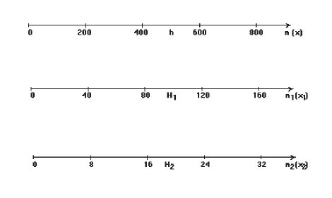
Fig. 2: Rescaled lattices.

If $n_{j}$ varies by one, $n$ varies by $N^{j}$, a number much larger than unity. For this reason, $n_{j}$ is a “slow variable” and provide an asymptotic behavior of the system. For each $j$ there is a slow lattice variable corresponding to the slow index $n_{j}$. $n_{j}$ will be an integer only if $n$ is a common multiple of $N^{j}$.

Let us consider $F_{n}$, a function of the discrete index $n$. An equation on the lattice is a functional relation which involves the function $F$ at various lattice points, $\{F_{n+\ell}\}$. In the case of the model considered before (2, 2), $\ell=\pm 1$. We are interested to transform the system, defined on a lattice $n$, to the slowly varying lattices $n_{j}$, providing the scales of the asymptotic behavior of the original system. This is equivalent to say that we are interested in transforming the system defined on $x$ to the one with the slowly varying variables $x_{j}$. We can consider the function $F_{n}$ written in terms of the slowly varying lattice variables $\{n_{j}\}$, with, for example, $j=1,2$, $F_{n}\equiv f_{n_{1},n_{2}},$ and we can carry out the $\epsilon$ expansion of the function $F_{n+\ell}$.

Let us consider at the beginning the case of one slowly varying lattice $n_{1}$, i.e. $F_{n}\equiv f_{n_{1}}$. As the shift operator $T_{n}$ acting on $F_{n}$ gives $T_{n}F_{n}=F_{n+1},$ we have $F_{n+\ell}=T_{n}^{\ell}F_{n}$. In order to extract the behaviour of the function $F_{n+1}=F(x+h)$ on the new scales, let us carry out the Taylor expansion of $F_{n+1}$ in powers of $h$. In such a case the shift operator can be expressed as an infinite order differential operator with respect to $x$, i.e.

$$T_{n}=\exp(h\partial_{x})=\sum_{k=0}^{\infty}\frac{(h\partial_{x})^{k}}{k!}.$$ (5)

Moreover, if we define a $\sl\Delta$ operator as $\Delta^{(+)}_{n}\equiv(T_{n}-1)/h$, we have

$$\partial_{x}=\frac{\log(1+h\Delta^{(+)}_{n})}{h},$$ (6)

and eq. (5) could be written as

$$T_{n}=\sum_{k=0}^{\infty}\frac{(\log(1+h\Delta^{(+)}_{n}))^{k}}{k!}.$$ (7)

Formulas (6, 7) are written in terms of $\Delta_{n}^{(+)}$. However on the lattice we can define an infinite number of different difference operators which in the continuum limit, when $h$ goes to zero, go over to the first order derivative. Among them it is important the asymmetric shift operator $\Delta_{n}^{(s)}\equiv\frac{1}{2h}(T_{n}-T_{n}^{-1})$. In this case we have

$$\partial_{x}=\frac{\mathrm{arcsinh}(h\Delta_{n}^{(s)})}{h},\quad\rightarrow\quad T_{n}=\sum_{k=0}^{\infty}\frac{(\mathrm{arcsinh}(h\Delta_{n}^{(s)}))^{k}}{k!}.$$ (8)

Introducing the slowly varying variable $x_{1}$ and the corresponding lattice $n_{1}$ in eq. (5), as $\partial_{x}=\epsilon\partial_{x_{1}}$, we have

$$T_{n}^{\ell}=e^{\ell h\partial_{x}}=e^{\ell\epsilon h\partial_{x_{1}}}=T_{n_{1}}^{\ell\epsilon}=\sum_{k=0}^{\infty}\frac{(\ell h\epsilon\partial_{x_{1}})^{k}}{k!}.$$ (9)

If we introduce more lattice variables, for example $\{n_{j}\}$, with $j=1,2$, then $T_{n}$ becomes

$$T_{n}^{\ell}=T_{n_{1}}^{\ell\epsilon}T_{n_{2}}^{\ell\epsilon^{2}}=\sum_{k=0}^{\infty}\frac{(\ell\epsilon h\partial_{x_{1}})^{k}}{k!}\sum_{j=0}^{\infty}\frac{(\ell\epsilon^{2}h\partial_{x_{2}})^{j}}{j!}.$$ (10)

Once we expand the operator $\partial_{x_{j}}$ in terms of shift operators we get an expression for $F(n\pm\ell)$ in terms of variations of $f(n_{1},n_{2})$ with coefficients depending on $\epsilon$ and $\ell$.

As delta operators are linear combinations of shift operators, from eq. (13) it can be proved [18, 24] that for $\Delta=\Delta^{(+)}$ we have the following formula

$$({\Delta}^{(+)}_{n_{1}})^{k}f_{n_{1}}=\sum_{i=k}^{\infty}\frac{k!}{i!}P(i,k)({\Delta}_{n}^{(+)})^{i}F_{n},$$ (11)

where $({\Delta}_{n_{1}}^{(+)})^{k}f_{n_{1}}$ is the $k$th-difference of $f_{n_{1}}$ respect to $n_{1}$, and the coefficients $P(i,k)$ are given by $P(i,j)=\sum_{\alpha=j}^{i}w^{\alpha}S_{i}^{\alpha}G_{\alpha}^{j},$ where $\omega$ is the ratio of the increment in the lattice of variable $n$ with respect to that of variable $n_{1}$. In this case, taking into account equation (4), $\omega$=$N$. The coefficients $S_{i}^{\alpha}$ and $G_{\alpha}^{j}$ are the Stirling coefficients of the first kind and second kind, respectively. The result (11) can be inverted, providing:

$$({\Delta}_{n}^{(+)})^{k}F_{n}=\sum_{i=k}^{\infty}\frac{k!}{i!}Q(i,k)({\Delta}^{(+)}_{n_{1}})^{i}f_{n_{1}},$$ (12)

where $Q(i,j)$ is the same as $P(i,j)$, but with $w=N^{-1}=\epsilon$.

A general way to get these formulas is provided by the finite operator calculus [30, 29, 13]. The finite operator calculus prescribes the following formula [25]

$$T_{n}^{j}=\sum_{k=0}^{\infty}\frac{(\epsilon)^{k}p_{k}(j)}{k!}(\Delta_{n_{1}})^{k},$$ (13)

where the functions $p_{k}(j)$ are the unique basic sequence associated to the operator $\Delta_{n_{1}}$, i.e. such that they satisfy the following conditions

$$p_{0}(n_{1})=1,\qquad p_{k}(0)=0\quad\mbox{for all}\quad k>0,$$ (14)

$$\Delta_{n_{1}}p_{k}(n_{1})=kp_{k-1}(n_{1}).$$

The basic sequences can be directly obtained by the transfer formulae:

$$p_{k}(n_{1})=n_{1}\bigl{(}\frac{\Delta_{n_{1}}}{h\partial_{x_{1}}}\bigr{)}^{-k}n{{}_{1}}^{k-1}.$$ (15)

When $\Delta_{n_{1}}=\Delta_{n_{1}}^{(+)}$ or $\Delta_{n_{1}}=\Delta_{n_{1}}^{(s)}$, the basic sequences are:

$$p_{k}^{(+)}(n_{1})=h^{k}n_{1}\bigl{(}\frac{e^{h\partial_{x_{1}}}-1}{h\partial_{x_{1}}}\bigr{)}^{-k}n{{}_{1}}^{k-1}=(x_{1})_{k}\equiv x_{1}(x_{1}-h)\cdots(x_{1}-kh+h),$$ (16)

$$p_{k}^{(s)}(n_{1})=h^{k}n_{1}\bigl{(}\frac{e^{h\partial_{x_{1}}}-e^{-h\partial_{x_{1}}}}{2h\partial_{x_{1}}}\bigr{)}^{-k}{n_{1}}^{k-1}=(2h)^{k}G_{k}(x_{1};-h,2h),$$

where $G_{k}(y;a,b)$ are the Gould polynomials [29] given by

$$G_{k}(y;a,b) {\equiv} \frac{y}{y-ka}\bigl{(}\frac{y-ka}{b}\bigr{)}_{k}$$

$$= \frac{y}{(y-ka)(b)^{k}}(y-ka)(y-ka-b)\cdots(y-ka-(k-1)b).$$

Let us also mention that for each $\Delta_{n_{1}}$ operator we can write from eq. (13)

$$(\partial_{x_{1}})^{j}=\frac{1}{h^{j}}\sum_{k=0}^{\infty}\frac{1}{k!}\bigl{[}\frac{\text{d}^{j}}{\text{d}y^{j}}p_{k}(y)\bigr{]}{\bigr{|}}_{y=0}(\Delta_{n_{1}})^{k},$$ (18)

i.e. we can express the partial derivative as an infinite sum of differences whose coefficients depends from the type of difference we are expanding into. In terms of $\Delta^{(+)}$, from eqs. (13, 16), eq. (9) reads

$$T_{n}^{\ell}F_{n}=\sum_{k=0}^{\infty}\frac{(h\epsilon)^{k}(\ell)_{k}}{k!}({\Delta}^{(+)}_{n_{1}})^{k}f_{n_{1}},$$ (19)

while, in the symmetric difference case, it reads

$$T_{n}^{\ell}F_{n}=\sum_{k=0}^{\infty}\frac{(2h\epsilon)^{k}}{k!}G_{k}(l;-1,2)({\Delta}^{(s)}_{n_{1}})^{k}f_{n_{1}}.$$ (20)

From eqs. (19,20) we get that any finite shift in the original equation will give rise to an expression in the slowly varying variables which involves an infinity of lattice points or, equivalently, contains differences at all orders of the function $f_{n_{1}}$. So to get a reduced equation on a finite number of points we need to cut the series by requiring that the function $f_{n_{1}}$ be of finite order of variation. Let us introduce the following definition:

$\mathbf{Definition:}$ The function $f_{n}$ is a slow varying function of order $p$ if

$$\Delta^{p+1}f_{n}=0.$$ (21)

Than we can prove the following Theorem:

$\bf{Theorem}$ The function $F_{n}$ is a slow varying function of order $p$ iff $f_{n_{1}}$ is a slowly varying function of order $p$ in its own variable, i.e. if $\Delta_{n_{1}}^{p+1}f_{n_{1}}=0$.

Proof.

The proof of this theorem will be given in the case of $\Delta=\Delta^{+}$, but it is easy to see that is valid for any delta operator. It is divided in two parts:

a) Be $f_{n_{1}}$ a slowly varying function of order $p$. From formula (12) it follows that

$${\Delta}_{n}^{p+1}F_{n}=\sum_{i=p+1}^{\infty}\frac{(p+1)!}{i!}Q(i,p+1){\Delta}_{n_{1}}^{i}f_{n_{1}}=0,$$ (22)

i.e. $F_{n}$ is also a slow function of order $p$.

b) Be $F_{n}$ a slowly varying function of order $p$. From formula (11) it follows that

$${\Delta}_{n_{1}}^{p+1}f_{n_{1}}=\sum_{i=p+1}^{\infty}\frac{(p+1)!}{i!}P(i,p+1){\Delta}_{n}^{i}F_{n}=0,$$ (23)

i.e. $f_{n_{1}}$ is also a slow function of order $p$.

∎

The expansion (20) can be performed in two steps: at first we write the shift operator in the $n$ variable in terms of the derivatives with respect to $x_{1}$ by formula (9) and then we expand the derivatives with respect to $x_{1}$ in term of delta operators by formula (18). In doing so we will have formulas in derivatives which are valid for any delta operator. Moreover the first expansion has $\epsilon$ dependent coefficients while the second will provide a finite number of terms only if we use the slow varying condition for the functions $f_{n_{1},n_{2}}$.

Let us now explicitate the first terms of eq. (20) for future use, at first in term of the derivatives and then in delta operators assuming that the function $f_{n_{1},n_{2}}$ is a slow function at most of order 2. At first we shall consider the case in which we have only one slow lattice, just the variable $n_{1}$ is present and then we extend the result to the case of two slow lattices, $n_{1}$ and $n_{2}$ and to partial lattices $n$ and $m$.

3.1.1 $F_{n}$=$f_{n_{1}}$=$f(x_{1})$

From Eq. (9) we get

$$F_{n\pm{1}}=f(x_{1})\pm h\epsilon\partial_{x_{1}}f(x_{1})+\frac{h^{2}\epsilon^{2}}{2!}\partial^{2}_{x_{1}}f(x_{1})+\mathcal{O}(\epsilon^{3}).$$ (24)

As from eq.(18) for $p$=2, $\partial_{x_{1}}$=$\Delta_{n_{1}}$ and ${\partial^{2}}_{x_{1}}$=$(\Delta_{n_{1}})^{2}$, then equation (24) reads

$$F_{n\pm{1}}=f_{n_{1}}\pm\frac{1}{2N}(f_{n_{1}+1}-f_{n_{1}-1})+\frac{1}{2N^{2}}(f_{n_{1}+1}-2f_{n_{1}}+f_{n_{1}-1})+O(N^{-3}).$$ (25)

3.1.2 $F_{n}$=$f_{n_{1},n_{2}}$=$f(x_{1},x_{2})$

$p$=2 is the lowest nontrivial value of $p$ for which we can consider $F_{n}$ as a function of the two scales, $n_{1}$ and $n_{2}$. Taking $l$=1, from eq. (10) we have

$$F_{n\pm 1} = f(x_{1},x_{2})\pm{h\epsilon}\frac{{\partial}f(x_{1},x_{2})}{\partial{x_{1}}}+\frac{h^{2}\epsilon^{2}}{2}\frac{{\partial^{2}}f(x_{1},x_{2})}{{\partial}x_{1}^{2}}\pm{h\epsilon^{2}}\frac{{\partial}f(x_{1},x_{2})}{\partial{x_{2}}}$$

$$+ {h^{2}\epsilon^{3}}\frac{\partial}{\partial{x_{1}}}\frac{{\partial}f(x_{1},x_{2})}{\partial{x_{2}}}+O(\epsilon^{4}).$$

If $F_{n}$ is a slowly varying function of order two in $n_{1}$, it might be of order one in $n_{2}$. In this case, eq. (3.1.2) becomes

$$F_{n\pm 1}=f(x_{1},x_{2})\pm{h\epsilon}\frac{{\partial}f(x_{1},x_{2})}{\partial{x_{1}}}+\frac{h^{2}\epsilon^{2}}{2}\frac{{\partial^{2}}f(x_{1},x_{2})}{{\partial}x_{1}^{2}}\pm{h\epsilon^{2}}\frac{{\partial}f(x_{1},x_{2})}{\partial{x_{2}}}+O(\epsilon^{3}).$$ (27)

Moreover, from eq. (18) it follows that $\partial_{x_{2}}$=$\Delta_{n_{2}}$, $\partial_{x_{1}}^{2}$=$(\Delta_{n_{1}})^{2}$ and $\partial_{x_{1}}\partial_{x_{2}}$ =$\Delta_{n_{1}}\Delta_{n_{2}}$. Then eqs. (3.1.2,27), written in terms of differences instead of derivatives, are given by

$$F_{n\pm 1} = f_{n_{1},n_{2}}\pm\frac{1}{2N}(f_{n_{1}+1,n_{2}}-f_{n_{1}-1,n_{2}})$$

$$+ \frac{1}{2N^{2}}(f_{n_{1}+1,n_{2}}-2f_{n_{1},n_{2}}+f_{n_{1}-1,n_{2}})\pm\frac{1}{2N^{2}}(f_{n_{1},n_{2}+1}-f_{n_{1},n_{2}-1})$$

$$+ \frac{1}{4N^{3}}(f_{n_{1}+1,n_{2}+1}-f_{n_{1}-1,n_{2}+1}-f_{n_{1}+1,n_{2}-1}+f_{n_{1}-1,n_{2}-1})+O(N^{-4})$$

and

$$F_{n\pm 1} = f_{n_{1},n_{2}}\pm\frac{1}{2N}(f_{n_{1}+1,n_{2}}-f_{n_{1}-1,n_{2}})$$

$$+ \frac{1}{2N^{2}}(f_{n_{1}+1,n_{2}}-2f_{n_{1},n_{2}}+f_{n_{1}-1,n_{2}})\pm\frac{1}{2N^{2}}(f_{n_{1},n_{2}+1}-f_{n_{1},n_{2}-1})+O(N^{-3}),$$

respectively.

3.1.3 $F_{n,m}$=$f_{n_{1},m_{1},m_{2}}$=$f(x_{1},t_{1},t_{2})$

In this case we have

$$F_{n,m\pm 1} = f(x_{1},t_{1},t_{2})\pm{\tau}\epsilon\frac{{\partial}f(x_{1},t_{1},t_{2})}{\partial{t_{1}}}$$

$$+ \frac{\tau^{2}\epsilon^{2}}{2}\frac{{\partial^{2}}f(x_{1},t_{1},t_{2})}{{\partial}t_{1}^{2}}\pm{\tau\epsilon^{2}}\frac{{\partial}f(x_{1},t_{1},t_{2})}{\partial{t_{2}}}+O(\epsilon^{3}),$$

and

$$F_{n\pm{1},m}=f(x_{1},t_{1},t_{2})\pm{h\epsilon}\frac{{\partial}f(x_{1},t_{1},t_{2})}{\partial{x_{1}}}+\frac{h^{2}\epsilon^{2}}{2}\frac{{\partial^{2}}f(x_{1},t_{1},t_{2})}{{\partial}x_{1}^{2}}+O(\epsilon^{3}).$$ (31)

In terms of differences, the last two equations are given by

$$F_{n,m\pm 1} = f_{n_{1},m_{1},m_{2}}\pm\frac{1}{2N}(f_{n_{1},m_{1}+1,m_{2}}-f_{n_{1},m_{1}-1,m_{2}})$$

$$+ \frac{1}{2N^{2}}(f_{n_{1},m_{1}+1,m_{2}}-2f_{n_{1},m_{1},m_{2}}+f_{n_{1},m_{1}-1,m_{2}})$$

$$\pm \frac{1}{2N^{2}}(f_{n_{1},m_{1},m_{2}+1}-f_{n_{1},m_{1},m_{2}-1})+O(N^{-3})$$

and

$$F_{n\pm{1},m} = f_{n_{1},m_{1},m_{2}}\pm\frac{1}{2N}(f_{n_{1}+1,m_{1},m_{2}}-f_{n_{1}-1,m_{1},m_{2}})$$

$$+ \frac{1}{2N^{2}}(f_{n_{1}+1,m_{1},m_{2}}-2f_{n_{1},m_{1},m_{2}}+f_{n_{1}-1,m_{1},m_{2}})+O(N^{-3}).$$

For future use we can further rescale the lattice with some extra parameter by defining $n_{1}=\frac{L_{1}n}{N}$, $m_{1}=\frac{L_{2}m}{N}$ and $m_{2}=\frac{m}{N^{2}}$, where the order 1 parameters $L_{1}$ and $L_{2}$ are divisors of $N$ and $N^{2}$ respectively if we require that $n_{1}$ and $n_{2}$ be integer numbers. In this case, the equations (3.1.3) and (31) become

$$F_{n,m\pm 1} = f(x_{1},t_{1},t_{2})\pm{{\tau}L_{2}\epsilon}\frac{{\partial}f(x_{1},t_{1},t_{2})}{\partial{t_{1}}}+\frac{\tau^{2}L_{2}^{2}\epsilon^{2}}{2}\frac{{\partial^{2}}f(x_{1},t_{1},t_{2})}{{\partial}t_{1}^{2}}$$

$$\pm {\tau\epsilon^{2}}\frac{{\partial}f(x_{1},t_{1},t_{2})}{\partial{t_{2}}}+O(\epsilon^{3}),$$

and

$$F_{n\pm{1},m}=f(x_{1},t_{1},t_{2})\pm{{h}L_{1}\epsilon}\frac{{\partial}f(x_{1},t_{1},t_{2})}{\partial{x_{1}}}+\frac{h^{2}L_{1}^{2}\epsilon^{2}}{2}\frac{{\partial^{2}}f(x_{1},t_{1},t_{2})}{{\partial}x_{1}^{2}}+O(\epsilon^{3}).$$ (35)

Moreover, from equation (3.1.3) we have

$$F_{n,m+1}-2F_{n,m}+F_{n,m-1}={\tau^{2}L_{2}^{2}\epsilon^{2}}\frac{{\partial^{2}}f(x_{1},t_{1},t_{2})}{{\partial}t_{1}^{2}}+O(\epsilon^{3}).$$ (36)

In terms of symmetric difference operators these equations can be written as

$$F_{n,m\pm 1} = f_{n_{1},m_{1},m_{2}}\pm\frac{L_{2}}{2N}(f_{n_{1},m_{1}+1,m_{2}}-f_{n_{1},m_{1}-1,m_{2}})$$

$$+ \frac{L_{2}^{2}}{2N^{2}}(f_{n_{1},m_{1}+1,m_{2}}-2f_{n_{1},m_{1},m_{2}}+f_{n_{1},m_{1}-1,m_{2}})$$

$$\pm \frac{1}{2N^{2}}(f_{n_{1},m_{1},m_{2}+1}-f_{n_{1},m_{1},m_{2}-1})+O(N^{-3}),$$

$$F_{n\pm{1},m} = f_{n_{1},m_{1},m_{2}}\pm\frac{L_{1}}{2N}(f_{n_{1}+1,m_{1},m_{2}}-f_{n_{1}-1,m_{1},m_{2}})$$

$$+ \frac{L_{1}^{2}}{2N^{2}}(f_{n_{1}+1,m_{1},m_{2}}-2f_{n_{1},m_{1},m_{2}}+f_{n_{1}-1,m_{1},m_{2}})+O(N^{-3})$$

and

$$F_{n,m+1}-2F_{n,m}+F_{n,m-1} = \frac{L_{2}^{2}}{N^{2}}(f_{n_{1},m_{1}+1,m_{2}}-2f_{n_{1},m_{1},m_{2}}+f_{n_{1},m_{1}-1,m_{2}})$$

$$+ O(N^{-3}).$$

The last three equations will be used in the following Section to apply the multiscale method to the biatomic lattice model we introduced in Section 2.

4 MULTISCALE REDUCTION OF THE DISCRETE BIATOMIC SYSTEM

4.1 Equations of motion

In the equations of motion of the biatomic chain (see eqs. (2,2)), the nonlinear terms (proportional to $\beta_{1}$ and $\beta_{2}$) are of order $\epsilon$ respect to the remaining terms, and thus we can use perturbative methods to look for approximate solutions of $x_{n}(t)$ and $y_{n}(t)$. This has been done in 1993 by Campa et al. [9] using the multiscale perturbative method with just the lowest order differential terms. In this way, performing at the same time a multiscale expansion and a continuum limit they were able to reduce the system to the NLSE (69).

Here we discretize time and look for completely discrete equations, i.e. passing from the differential terms in the expansion (see eqs. (24, 3.1.2, 27, 3.1.3, 31, 3.1.3–36)) to difference terms corresponding to the lowest order of slow varyness $p$, i.e. to eqs. (25, 3.1.2, 3.1.2, 3.1.3, 3.1.3, 3.1.3–3.1.3). To discretize time we replace the time $t$ with a discrete variable $m$, so that $t$$\equiv$$m\tau$, where $\tau$ is the temporal scale. Thus, when $\tau$ reduces to an infinitesimal quantity and $m$ approaches infinity in such a way that $t$ remains finite we recover the continuous case. We consider the simplest approximation of the second derivative by differences using a central difference so as to get a real dispersive relation. The discretized equations of motion are given by

$$m_{1}(x_{n,m+1}-2x_{n,m}+x_{n,m-1}) = k_{1}(y_{n,m}-x_{n,m})-k_{2}(x_{n,m}-y_{n-1,m})$$

$$+ \epsilon[\beta_{1}(y_{n,m}-x_{n,m})^{2}-\beta_{2}(x_{n,m}-y_{n-1,m})^{2}],$$

$$m_{2}(y_{n,m+1}-2y_{n,m}+y_{n,m-1}) = -k_{1}(y_{n,m}-x_{n,m})+k_{2}(x_{n+1,m}-y_{n,m})$$

$$- \epsilon[\beta_{1}(y_{n,m}-x_{n,m})^{2}-\beta_{2}(x_{n+1,m}-y_{n,m})^{2}],$$

where $x_{n,m}$$\equiv$$x_{n}(m\tau)$, $y_{n,m}$$\equiv$$y_{n}(m\tau)$ and $m_{1,2}$$\equiv$$\frac{M_{1,2}}{\tau^{2}}$. We are looking for $x_{n,m}$ and $y_{n,m}$ as bounded solutions written as a modulation of the harmonic wave solutions of the linearized equations which one obtains when setting $\epsilon=0$. The harmonic waves are given by

$$E_{n,m}=e^{i[kn-{\omega}(k)m]},$$ (42)

with $\omega(k)$ real for any real value of $k$. The physical reason for choosing harmonic waves is that the atoms of the chain make only small oscillations around their equilibrium position. When we introduce this ansatz into equations (4.1) and (4.1), we realize at once that the solution of the nonlinear equations of motion can be represented as a modulated linear combination of harmonic functions.

A solution of the linear part of eqs. (4.1) and (4.1) ($\beta_{1}$=$\beta_{2}$=0), written in terms of the harmonic waves (42), is given by

$$x_{n,m}=A\,E_{n,m},\qquad y_{n,m}=B\,E_{n,m},$$

where

$$\frac{B}{A}=r{\equiv}\frac{k_{1}+k_{2}+2m_{1}(\cos{\omega(k)}-1)}{k_{1}+k_{2}e^{-ik}}=\frac{k_{1}+k_{2}e^{ik}}{k_{1}+k_{2}+2m_{2}(\cos{\omega(k)}-1)},$$ (43)

with the dispersion relation

$$\omega(k)={\scriptstyle\arccos\{1-\frac{1}{4m_{1}m_{2}}\bigl{[}(k_{1}+k_{2})(m_{1}+m_{2})\pm\sqrt{(k_{1}+k_{2})^{2}(m_{1}+m_{2})^{2}-16k_{1}k_{2}m_{1}m_{2}{sin}^{2}\frac{k}{2}}\bigr{]}\}}.$$ (44)

It can be proved that the term inside the square root of the dispersion relation is always positive, so that the argument of “arccos” is always real.

Fig. 3: Graph of $\omega(k)$ against $k$, with $k$ lying in the interval [0,$\pi$]. We have chosen $M_{1}$=1, $M_{2}$=1.5, $k_{1}$=1, $k_{2}$=0.3 and $\tau$=$10^{-1/2}$.

Fig. 4: Graph of $\omega(k)$ against $k$, with $k$ lying in the interval [0,$\pi$]. The parameters $M_{1}$, $M_{2}$, $k_{1}$, and $k_{2}$ are the same as in Fig. 4, but $\tau$=$\tau_{o}$.

In equation (44), the positive sign corresponds to the optical branch $\omega_{opt}(k)$, whereas the negative one to the acoustical branch $\omega_{ac}(k)$. It can be proved that the function $\omega(k)$ is real for all real values of $k$ iff the temporal scale $\tau$ satisfies the following inequalities:

$$\tau{\leq}\sqrt{\frac{4M_{1}M_{2}}{(k_{1}+k_{2})(M_{1}+M_{2})}}\equiv\tau_{o}$$ (45)

for the optical branch, and

$$\tau{\leq}\sqrt{\frac{8M_{1}M_{2}}{(k_{1}+k_{2})(M_{1}+M_{2})-\sqrt{(k_{1}+k_{2})^{2}(M_{1}+M_{2})^{2}-16k_{1}k_{2}M_{1}M_{2}}}}{\equiv}\tau_{a}$$ (46)

for the acoustical one. It is easy to show that $\tau_{a}$ is always larger than $\tau_{o}$. In Figs. (3, 4) we show how $\omega(k)$ varies as a function of $\tau$. We have chosen, following Campa[9] , the following numerical values for the parameters, $M_{1}$=1, $M_{2}$=1.5, $k_{1}$=1 and $k_{2}$=0.3, so that $\tau_{o}$$\simeq$1.358732 and $\tau_{a}$$\simeq$2.910816. So the obtained threshold values $\tau_{o}$ and $\tau_{a}$ are consistent with the request that $\tau$, the discretization parameter, be smaller than one.

Let us seek a finite amplitude solution of the nonlinear system (4.1, 4.1). To do so, we write $x_{n,m}$ and $y_{n,m}$ in terms of the harmonics of the linearized equation (42)

$$x_{n,m} = \sum_{s=0}^{\infty}G_{n,m}^{s}(E_{n,m})^{s}+\sum_{s=1}^{\infty}\bar{G}_{n,m}^{s}(E_{n,m})^{-s},$$ (47)

$$y_{n,m} = \sum_{s=0}^{\infty}H_{n,m}^{s}(E_{n,m})^{s}+\sum_{s=1}^{\infty}\bar{H}_{n,m}^{s}(E_{n,m})^{-s},$$ (48)

where, as the variables $x_{n,m}$ and $y_{n,m}$ are real, ($\bar{G}_{n,m}^{s}$, $\bar{H}_{n,m}^{s}$) are the complex conjugates of the modulation coefficients ($G_{n,m}^{s}$, $H_{n,m}^{s}$). We choose $G_{n,m}^{s}$=$g_{n_{1},m_{1},m_{2}}^{s}$ and $H_{n,m}^{s}$=$h_{n_{1},m_{1},m_{2}}^{s}$ as slowly varying functions of the second order in $n_{1}$ and $m_{1}$ and of the first order in $m_{2}$, defined in such a way to avoid secular terms. Moreover we expand the functions $g_{n_{1},m_{1},m_{2}}^{s}$ and $h_{n_{1},m_{1},m_{2}}^{s}$ in the small parameter $\epsilon$. So we have:

$$G_{n,m}^{s} \equiv \sum_{l=0}^{\infty}\epsilon^{l}g_{n_{1},m_{1},m_{2}}^{(s,l)},$$ (49)

$$H_{n,m}^{s} \equiv \sum_{l=0}^{\infty}\epsilon^{l}h_{n_{1},m_{1},m_{2}}^{(s,l)}.$$ (50)

4.2 Derivation of the equations of motion

Substituting ansatz (47, 48) into the equations of motion (4.1, 4.1) and taking into account eqs. (49, 50) we get two equations of the form

$$\sum_{s=0}^{\infty}\sum_{l=0}^{\infty}\epsilon^{l}F_{n_{1},m_{1},m_{2}}^{(s,l)}(E_{n,m})^{s}+\sum_{s=0}^{\infty}\sum_{l=0}^{\infty}\epsilon^{l}\bar{F}_{n_{1},m_{1},m_{2}}^{(s,l)}(E_{n,m})^{-s}=0,$$ (51)

where the $F_{n_{1},m_{1},m_{2}}^{(s,l)}$ are function only of the slow variables. As $(E_{n,m})^{s}$ and $(E_{n,m})^{-s}$ are independent functions, its coefficients must be equal to zero. So for each power of $(E_{n,m})$ and $\epsilon$ we get sets of equations $F_{n_{1},m_{1},m_{2}}^{(s,l)}=0$ for the slow varying modulation coefficients $g_{n_{1},m_{1},m_{2}}^{(s,l)}$ and $h_{n_{1},m_{1},m_{2}}^{(s,l)}$ together with their complex conjugate.

4.2.1 $\epsilon^{0}$

We look here for the linearized terms. In this case, the coefficient of the zeroth harmonic satisfies the equation

$$g_{n_{1},m_{1},m_{2}}^{(0,0)}=h_{n_{1},m_{1},m_{2}}^{(0,0)},$$ (52)

whereas the coefficients of the first harmonics gives a set of two equations that are identically satisfied when $\omega(k)$ satisfies the dispersion relation (44) and

$$\frac{h_{n_{1},m_{1},m_{2}}^{(1,0)}}{g_{n_{1},m_{1},m_{2}}^{(1,0)}}=r.$$ (53)

It can be proven easily that, for $q$$\geq$2, $g_{n_{1},m_{1},m_{2}}^{(q,0)}$=$h_{n_{1},m_{1},m_{2}}^{(q,0)}$=0.

4.2.2 $\epsilon^{1}$

The coefficients of the zeroth harmonic are

$$h^{(0,1)}(x_{1},t_{1},t_{2}) = g^{(0,1)}(x_{1},t_{1},t_{2})+\frac{hL_{1}k_{2}}{k_{1}+k_{2}}\frac{{\partial}g^{(0,0)}(x_{1},t_{1},t_{2})}{{\partial}x_{1}}$$

$$+ \frac{2}{k_{1}+k_{2}}[\beta_{2}|1-e^{-ik}r|^{2}-\beta_{1}|1-r|^{2}]|g^{(1,0)}(x_{1},t_{1},t_{2})|^{2},$$

or

$$h_{n_{1},m_{1},m_{2}}^{(0,1)} = g_{n_{1},m_{1},m_{2}}^{(0,1)}+\frac{L_{1}k_{2}}{2(k_{1}+k_{2})}(g_{n_{1}+1,m_{1},m_{2}}^{(0,0)}-g_{n_{1}-1,m_{1},m_{2}}^{(0,0)})$$

$$+ \frac{2}{k_{1}+k_{2}}[\beta_{2}|1-e^{-ik}r|^{2}-\beta_{1}|1-r|^{2}]|g_{n_{1},m_{1},m_{2}}^{(1,0)}|^{2},$$

depending if we use the expansions in terms of derivatives or differences.

For $s$=1 we find a system of two equations in the two unknowns $g_{n_{1},m_{1},m_{2}}^{(1,1)}$ and $h_{n_{1},m_{1},m_{2}}^{(1,1)}$. This system is compatible only if

$$g_{n_{1},m_{1},m_{2}}^{(1,0)}{\equiv}g_{n_{2},m_{2}}^{(1,0)},$$ (56)

where $n_{2}=n_{1}-m_{1}$ and

$$h_{n_{1},m_{1},m_{2}}^{(1,1)}=rg_{n_{1},m_{1},m_{2}}^{(1,1)}+\frac{2i\sin{\omega}m_{1}\omega_{,k}+k_{2}re^{-ik}}{2(k_{1}+k_{2}e^{-ik})}L_{1}(g_{n_{2}+1,m_{2}}^{(1,0)}-g_{n_{2}-1,m_{2}}^{(1,0)}),$$ (57)

where $\omega_{,k}$$\equiv$$\frac{\text{d}\omega}{\text{d}k}$ =$\frac{L_{2}}{L_{1}}$, with $L_{1}$ and $L_{2}$ given in Appendix A.1 by eqs. (72) and (73). The differential version of eq. (56) is

$$g^{(1,0)}(x_{1},t_{1},t_{2}){\equiv}g^{(1,0)}(x_{2},t_{2}),$$

where $x_{2}$$\equiv$$h$$n_{2}$=$h$($n_{1}-m_{1}$)=$x_{1}-{\frac{h}{\tau}}t_{1}$, and

$$h^{(1,1)}(x_{1},t_{1},t_{2})=rg^{(1,1)}(x_{1},t_{1},t_{2})+\frac{2i\sin{\omega}m_{1}\omega_{,k}+k_{2}re^{-ik}}{k_{1}+k_{2}e^{-ik}}hL_{1}\frac{{\partial}g(x_{2},t_{2})^{(1,0)}}{\partial{x_{2}}}.$$ (58)

For the second harmonic we get

$$g_{n_{1},m_{1},m_{2}}^{(2,1)} = K_{1}g_{n_{1},m_{1},m_{2}}^{(1,0){2}},$$ (59)

$$h_{n_{1},m_{1},m_{2}}^{(2,1)} = K_{2}g_{n_{1},m_{1},m_{2}}^{(1,0){2}},$$ (60)

where $K_{1}$ and $K_{2}$ are given in Appendix A.1 by eqs. (1, 1). It can be easily proven that, for $q$$\geq$3, $g_{n_{1},m_{1},m_{2}}^{(q,1)}$=$h_{n_{1},m_{1},m_{2}}^{(q,1)}$=0.

4.2.3 $\epsilon^{2}$

Taking into account eq. (56), the zeroth harmonic gives a system of two equations that is satisfied only if

$$\begin{array}[]{c}L_{1}^{2}(g_{n_{2}+1,m_{2}}^{(0,0)}+g_{n_{2}-1,m_{2}}^{(0,0)}-2g_{n_{2},m_{2}}^{(0,0)})=L_{1}\frac{c^{0}}{2}(|g_{n_{2}+1,m_{2}}^{(1,0)}|^{2}-|g_{n_{2}-1,m_{2}}^{(1,0)}|^{2})\\ +L_{1}\frac{c^{1}}{2}\{g_{n_{2},m_{2}}^{(1,0)}(\bar{g}_{n_{2}+1,m_{2}}^{(1,0)}-\bar{g}_{n_{2}-1,m_{2}}^{(1,0)})+\bar{g}_{n_{2},m_{2}}^{(1,0)}(g_{n_{2}+1,m_{2}}^{(1,0)}-g_{n_{2}-1,m_{2}}^{(1,0)})\},\end{array}$$ (61)

where $c^{0}$ and $c^{1}$ are two real constants given in Appendix A.3. Defining

$$A_{n_{2},m_{2}} {\equiv} L_{1}(g_{n_{2}+1,m_{2}}^{(0,0)}-g_{n_{2},m_{2}}^{(0,0)})-\frac{c^{0}}{2}(|g_{n_{2}+1,m_{2}}^{(1,0)}|^{2}+|g_{n_{2},m_{2}}^{(1,0)}|^{2})$$

$$- \frac{c^{1}}{2}(g_{n_{2},m_{2}}^{(1,0)}\bar{g}_{n_{2}+1,m_{2}}^{(1,0)}+\bar{g}_{n_{2},m_{2}}^{(1,0)}g_{n_{2}+1,m_{2}}^{(1,0)}),$$

eq. (61) reads:

$$A_{n_{2}+1,m_{2}}-A_{n_{2},m_{2}}=0.$$ (63)

Thus $A_{n_{2},m_{2}}=C(m_{2})$, where $C(m_{2})$ is an arbitrary function of $m_{2}$. Using the fact that $g_{n_{2},m_{2}}^{(0,0)}$ is a slowly varying function in $n_{2}$ we have

$$\begin{array}[]{c}L_{1}(g_{n_{2}+1,m_{2}}^{(0,0)}-g_{n_{2}-1,m_{2}}^{(0,0)})=c^{0}(|g_{n_{2}+1,m_{2}}^{(1,0)}|^{2}+|g_{n_{2},m_{2}}^{(1,0)}|^{2})\\ +c^{1}(g_{n_{2},m_{2}}^{(1,0)}\bar{g}_{n_{2}+1,m_{2}}^{(1,0)}+\bar{g}_{n_{2},m_{2}}^{(1,0)}g_{n_{2}+1,m_{2}}^{(1,0)})+C(m_{2}).\end{array}$$ (64)

Eq. (64) written in terms of the derivatives reads:

$$\begin{array}[]{c}hL_{1}\frac{{\partial}g^{(0,0)}(x_{2},t_{2})}{\partial{x_{2}}}=(c^{0}+c^{1})|g_{n_{2},m_{2}}^{(1,0)}|^{2}+\frac{C(m_{2})}{2}.\end{array}$$ (65)

If we transform the derivatives of eq. (65) into differences (using again eq. (18), and recalling that $x_{2}$=$h$$n_{2}$), we have

$$\begin{array}[]{c}L_{1}(g_{n_{2}+1,m_{2}}^{(0,0)}-g_{n_{2}-1,m_{2}}^{(0,0)})=2(c^{0}+c^{1})|g_{n_{2},m_{2}}^{(1,0)}|^{2}+C(m_{2}),\end{array}$$ (66)

an equation simpler than eq. (64). This difference is due to the fact that eq. (65) is obtained using the Leibniz’s rule and an integration, while in the case of eq. (64) the Leibniz’s rule is not applicable as we deal with differences.

Finally, for $s$=1, we get a system of two equations in the two unknowns, $g_{n_{2},m_{2}}^{(1,2)}$ and $h_{n_{2},m_{2}}^{(1,2)}$, which is compatible and not–secular only if

$$\begin{array}[]{c}iB_{1}(g_{n_{2},m_{2}+1}^{(1,0)}-g_{n_{2},m_{2}-1}^{(1,0)})+B_{2}L_{1}^{2}(g_{n_{2}+1,m_{2}}^{(1,0)}+g_{n_{2}-1,m_{2}}^{(1,0)}-2g_{n_{2},m_{2}}^{(1,0)})\\ +B_{3}|g_{n_{2},m_{2}}^{(1,0)}|^{2}g_{n_{2},m_{2}}^{(1,0)}+\{B_{4}(|g_{n_{2}+1,m_{2}}^{(1,0)}|^{2}+|g_{n_{2},m_{2}}^{(1,0)}|^{2})\\ +B_{5}(g_{n_{2},m_{2}}^{(1,0)}\bar{g}_{n_{2}+1,m_{2}}^{(1,0)}+\bar{g}_{n_{2},m_{2}}^{(1,0)}g_{n_{2}+1,m_{2}}^{(1,0)})+B_{6}C(m_{2})\}g_{n_{2},m_{2}}^{(1,0)}=0.\end{array}$$ (67)

Here the coefficients $B_{i}$ ($i$=1,…,6) are real and given in Appendix A.3. This is a NLSE on the lattice. At difference from the standard discrete–time NLS equation presented by Ablowitz and Ladik [1], this is completely local but not integrable [28, 39]. In the development of $x_{n,m}$ and $y_{n,m}$, $g^{(1,0)}_{n_{2},m_{2}}$ is the main term which multiplies $\epsilon^{0}$ and $E_{n,m}$. If we require that $g_{n_{2},m_{2}}^{(s,l)}$ and $h_{n_{2},m_{2}}^{(s,l)}$ are localized with respect to $n_{2}$, we have to set $C(m_{2})=0$ and eq. (67) becomes

$$\begin{array}[]{c}iB_{1}(g_{n_{2},m_{2}+1}^{(1,0)}-g_{n_{2},m_{2}-1}^{(1,0)})+B_{2}L_{1}^{2}(g_{n_{2}+1,m_{2}}^{(1,0)}+g_{n_{2}-1,m_{2}}^{(1,0)}-2g_{n_{2},m_{2}}^{(1,0)})\\ +B_{3}|g_{n_{2},m_{2}}^{(1,0)}|^{2}g_{n_{2},m_{2}}^{(1,0)}+\{B_{4}(|g_{n_{2}+1,m_{2}}^{(1,0)}|^{2}+|g_{n_{2},m_{2}}^{(1,0)}|^{2})\\ +B_{5}(g_{n_{2},m_{2}}^{(1,0)}\bar{g}_{n_{2}+1,m_{2}}^{(1,0)}+\bar{g}_{n_{2},m_{2}}^{(1,0)}g_{n_{2}+1,m_{2}}^{(1,0)})\}g_{n_{2},m_{2}}^{(1,0)}=0.\end{array}$$ (68)

5 CONTINUUM LIMIT OF THE DISCRETE NLS

Eq. (68) is obtained from eqs. (4.1, 4.1) by discretizing the continuous time variable. This discretization was necessary to be able to solve the $l=1$, $s=1$ system which otherwise would have been an unsolvable linear differential difference wave equation. By discretizing we get a discrete wave equation whose general solution is given by an arbitrary function of a discrete variable.

It is interesting to perform the limit when the discrete time $m_{1}$ is transformed into a continuous $t$–variable. To do so, we take the limit when $\tau$ goes to zero and $m$ tends to $\infty$ in such a way that the product $\tau m=t$ is finite. So eq. (68) becomes the integrable NLSE

$$iA_{1}\frac{{\partial}g^{(1,0)}(z_{2},t_{2})}{{\partial}t_{2}}+A_{2}\frac{\partial^{2}g^{(1,0)}(z_{2},t_{2})}{\partial{z_{2}}^{2}}+[A_{3}|g^{(1,0)}(z_{2},t_{2})|^{2}+A_{4}C(t_{2})]g^{(1,0)}(z_{2},t_{2})=0,$$ (69)

where $t_{2}$=$\lim_{\tau\rightarrow{0}}\lim_{m\rightarrow{\infty}}\tau{m_{2}}$ and $z_{2}$=$\frac{1}{N}(n_{1}-\frac{\text{d}\Omega}{\text{d}k}t_{1})$ is a new continuous variable. The coefficients $A_{i}$ ($i$=1,…,4) in this limit are finite and real, and are given by

$$A_{1} = \lim_{\tau\rightarrow{0}}2{\tau}B_{1}=-\Omega\frac{(M_{1}+M_{2})(k_{1}+k_{2})-2M_{1}M_{2}\Omega^{2}}{k_{1}+k_{2}-M_{2}\Omega^{2}},$$

$$A_{2} = \lim_{\tau\rightarrow{0}}B_{2}={\scriptstyle\frac{[(M_{1}+M_{2})(k_{1}+k_{2})-M_{1}M_{2}\Omega^{2})](\Omega_{,k})^{2}-M_{1}M_{2}(\Omega_{,k})^{2}-k_{1}k_{2}\cos{k}}{k_{1}+k_{2}-M_{2}\Omega^{2}}},$$

$$A_{3} = \lim_{\tau\rightarrow{0}}(B_{3}+2B_{4}+2B_{5})=\lim_{\tau\rightarrow{0}}(B_{3}+2(c_{0}+c_{1})B_{6})$$

$$= -{\scriptstyle 2\beta_{1}^{2}(\bar{R}-1)\{(R-1)|R-1|^{2}\frac{2k_{2}(1-\cos{k})-(M_{1}+M_{2})\Omega^{2}}{D}+\frac{2(R-1)}{k_{1}+k_{2}}|1-R|^{2}\}}$$

$$+ {\scriptstyle 2\beta_{2}^{2}(1-\bar{R}e^{ik})\{-(1-Re^{-ik})|1-Re^{-ik}|^{2}\frac{2k_{1}(1-\cos{k})-(M_{1}+M_{2})\Omega^{2}}{D}+\frac{2(Re^{-ik}-1)}{k_{1}+k_{2}}|1-Re^{-ik}|^{2}\}}$$

$$+ 2\beta_{1}\beta_{2}(\bar{R}-1)\{(\bar{R}-1)(1-Re^{-ik})^{2}\frac{(M_{2}+M_{1}e^{2ik})\Omega^{2}}{D}$$

$$+ {\scriptstyle\frac{2(R-1)}{k_{1}+k_{2}}|1-Re^{-ik}|^{2}\}+2\beta_{1}\beta_{2}(1-\bar{R}e^{ik})\{(R-1)^{2}(1-\bar{R}e^{ik})\frac{(M_{2}+M_{1}e^{-2ik})\Omega^{2}}{D}}$$

$$+ \frac{2(1-Re^{-ik})}{k_{1}+k_{2}}|1-R|^{2}\}+2gA_{4},$$

$$A_{4} = \lim_{\tau\rightarrow{0}}B_{6}=\frac{k_{1}\beta_{2}|1-Re^{-ik}|^{2}+k_{2}\beta_{1}|1-R|^{2}}{k_{1}+k_{2}},$$

where

$$g=\lim_{\tau\rightarrow{0}}(c_{1}+c_{2})\frac{2\beta_{2}k_{1}|1-Re^{-ik}|^{2}+2\beta_{1}k_{2}|1-R|^{2}}{(M_{1}+M_{2})(k_{1}+k_{2})(\Omega_{,k})^{2}-k_{1}k_{2}},$$

$$D=[k_{1}+k_{2}-M_{1}\Omega^{2}][k_{1}+k_{2}-M_{2}\Omega^{2}]-(k_{1}^{2}+k_{2}^{2}+2k_{1}k_{2}\cos{2k}),$$ (70)

and

$$R=\lim_{\tau\rightarrow{0}}r=\frac{k_{1}+k_{2}-M_{1}\Omega^{2}}{k_{1}+k_{2}e^{-ik}}.$$

$\Omega(k)$=$\lim_{\tau\rightarrow{0}}\frac{\omega(k)}{\tau}$ gives back the continuous dispersion relation [9].

6 CONCLUSIONS

In this work, introducing the concepts necessary for applying the perturbative multiscale method to discrete equations we have obtained a rescaled discrete equation. We have applied this technique to a biatomic chain model. In this way we have shown that we can perform in a coherent way a multiscale expansion on the lattice. If we want to remain on the lattice and want to avoid nonlocality then we need to restrict ourselves to slow–varying functions. This restriction on the class of function implies that some of the properties of the starting system will be lost. Among them by sure that of the integrability, which is strictly related to the analytic properties of the solutions.

We have found that $g^{(1,0)}$ (the slowly varying coefficient of the first harmonic) satisfies a totally discrete local version of the discrete NLSE. One interesting feature of our discrete NLSE is that, when we perform the continuous limit in the time variable, the spatial variable becomes continuous, and we get the continuous integrable NLSE (69) as in the work by Campa et al. [9].

Appendix A Explicit Formulas

A.1 $g_{n_{2},m_{2}}^{(1,1)}$ and $h_{n_{2},m_{2}}^{(1,1)}$

Let us consider the expansion of the equations of motion with $l$=$s$=1. In this case we get a system of two equations in two unknowns, $g_{n_{1},m_{1},m_{2}}^{(1,1)}$ and $h_{n_{1},m_{1},m_{2}}^{(1,1)}$, that is compatible only if

$$\begin{array}[]{c}[(k_{1}+k_{2})(m_{1}+m_{2})+4m_{1}m_{2}(\cos{\omega}-1)]\sin(\omega)L_{2}(g_{n_{1},m_{1}+1,m_{2}}^{(1,0)}-\\ -g_{n_{1},m_{1}-1,m_{2}}^{(1,0)})+k_{1}k_{2}\sin{k}L_{1}(g_{n_{1}+1,m_{1},m_{2}}^{(1,0)}-g_{n_{1}-1,m_{1},m_{2}}^{(1,0)})=0.\end{array}$$ (71)

It is convenient to choose

$$L_{1}=S\sin(\omega)[(k_{1}+k_{2})(m_{1}+m_{2})+4m_{1}m_{2}(\cos{\omega}-1)]$$ (72)

and

$$L_{2}=Sk_{1}k_{2}\sin{k},$$ (73)

where $S$ is a real number such that $L_{1}$ ($L_{2}$) is an integer number. In terms of $L_{1}$ and $L_{2}$ the dispersion relation becomes ${\omega}_{,k}=\frac{L_{2}}{L_{1}}.$ With this choice of $L_{1}$ and $L_{2}$, and assuming that $g_{n_{1},m_{1},m_{2}}^{(1,0)}=g_{n_{2},m_{2}}^{(1,0)}$, with $n_{2}$$\equiv$$n_{1}-m_{1}$, we find that eq. (71) is satisfied. Thus the system of equations we are studying is compatible, and leads us to the eq. (57).

A.2 The discrete NLSE

In this Appendix, we show the steps necessary to find the discrete NLSE (68). First, we take the equations of motion, and select the harmonic $s$=1 with $l$=2. In this way we get a system of two equations in the two unknowns $g_{n_{2},m_{2}}^{(1,2)}$ and $h_{n_{2},m_{2}}^{(1,2)}$, which is compatible only if the nonhomogeneous first order difference equation

$$\begin{array}[]{c}[(k_{1}+k_{2})(m_{1}+m_{2})+4m_{1}m_{2}(\cos{\omega}-1)]\sin(\omega)L_{2}(g_{n_{1},m_{1}+1,m_{2}}^{(1,1)}\\ -g_{n_{1},m_{1}-1,m_{2}}^{(1,1)})+k_{1}k_{2}\sin{k}L_{1}(g_{n_{1}+1,m_{1},m_{2}}^{(1,1)}-g_{n_{1}-1,m_{1},m_{2}}^{(1,1)})\\ =F(g_{n_{2}+1,m_{2}}^{(0,0)},g_{n_{2}-1,m_{2}}^{(0,0)},g_{n_{2},m_{2}}^{(1,0)}),\end{array}$$ (74)

is satisfied. Here $F$$\equiv$$F(g_{n_{2}\pm{1},m_{2}}^{(0,0)},g_{n_{2},m_{2}}^{(1,0)})$ is a given nonhomogeneous term. As the l.h.s. of this equation is the same as that of eq. (71) (but with $g_{n_{2}\pm{1},m_{2}}^{(1,1)}$ replaced by $g_{n_{2}\pm{1},m_{2}}^{(1,0)}$), the terms depending on $g^{(1,0)}$ contained in $F$ lead to secular terms for the unknown $g^{(1,1)}$. To avoid secular terms, we must set $F$=0 and eq. (74) gives $g_{n_{1},m_{1},m_{2}}^{(1,1)}$=$g_{n_{2},m_{2}}^{(1,1)}$.

If we substitute $g^{(0,0)}$ given by eq. (64) into $F$=0, then this condition will give eq. (68) written in terms of $g^{(1,0)}$.

A.3 Constants

We give here the expressions of the coefficients appearing in eqs. (59, 60, 64, 68):

1. Eqs. (59, 60).

   $$K_{1} \equiv \{\beta_{1}(r-1)^{2}[k_{1}+k_{2}e^{ik}-r(k_{1}+k_{2}e^{-2ik})]$$

   $$- \beta_{2}(1-re^{-ik})^{2}[k_{1}+k_{2}e^{ik}-r(k_{1}e^{2ik}+k_{2})]\}/\{rD\},$$

   $$K_{2} \equiv \{\beta_{1}(r-1)^{2}[k_{1}+k_{2}e^{2ik}-r(k_{1}+k_{2}e^{-ik})]$$

   $$- \beta_{2}(1-re^{-ik})^{2}[k_{1}+k_{2}e^{2ik}-r(k_{1}e^{2ik}+k_{2}e^{ik})]\}/\{D\},$$

   where

   $$D = [2m_{1}(\cos{2\omega}-1)+k_{1}+k_{2}][2m_{2}(\cos{2\omega}-1)+k_{1}+k_{2}]$$

   $$- (k_{1}^{2}+k_{2}^{2}+2k_{1}k_{2}\cos{2k}).$$

2. Eq. (64):

   $$c^{0}\equiv\frac{-2k_{2}[\beta_{2}|1-re^{-ik}|^{2}+\beta_{1}|1-r|^{2}]}{(m_{1}+m_{2})(k_{1}+k_{2})(\omega_{,k})^{2}-k_{1}k_{2}},$$

   $$c^{1}\equiv\frac{2\beta_{2}(k_{1}+k_{2})|1-re^{-ik}|^{2}}{(m_{1}+m_{2})(k_{1}+k_{2})(\omega_{,k})^{2}-k_{1}k_{2}}.$$

3. Eq. (68):

   $$B_{1} = -\sin{(\omega)}\frac{(m_{1}+m_{2})(k_{1}+k_{2})+4m_{1}m_{2}(\cos{\omega}-1)}{2m_{2}(\cos{\omega}-1)+k_{1}+k_{2}},$$

   $$B_{2} = {\scriptstyle\frac{[(m_{1}+m_{2})(k_{1}+k_{2})+4m_{1}m_{2}(\cos{\omega}-1)]\cos(\omega)(\omega_{,k})^{2}-m_{1}m_{2}{sin}^{2}(\omega)(\omega_{,k})^{2}-k_{1}k_{2}\cos{k}}{k_{1}+k_{2}+2m_{2}(\cos{\omega}-1)}},$$

   $$B_{3} = -{\scriptstyle 2\beta_{1}^{2}(\bar{r}-1)\{(r-1)|r-1|^{2}\frac{2k_{2}(1-\cos{k})+2(m_{1}+m_{2})(\cos{\omega}-1)}{D}}$$

   $$+ \frac{2(r-1)}{k_{1}+k_{2}}|1-r|^{2}\}$$

   $$+ {\scriptstyle 2\beta_{2}^{2}(1-\bar{r}e^{ik})\{-(1-re^{-ik})|1-re^{-ik}|^{2}\frac{2k_{1}(1-\cos{k})+2(m_{1}+m_{2})(\cos{\omega}-1)}{D}}$$

   $$+ \frac{2(re^{-ik}-1)}{k_{1}+k_{2}}|1-re^{-ik}|^{2}\}$$

   $$+ {\scriptstyle 2\beta_{1}\beta_{2}(\bar{r}-1)\{(\bar{r}-1)(1-re^{-ik})^{2}\frac{-2e^{2ik}m_{1}(\cos{\omega}-1)-2m_{2}(\cos{\omega}-1)}{D}}$$

   $$+ \frac{2(r-1)}{k_{1}+k_{2}}|1-re^{-ik}|^{2}\}$$

   $$+ {\scriptstyle 2\beta_{1}\beta_{2}(1-\bar{r}e^{ik})\{(r-1)^{2}(1-\bar{r}e^{ik})\frac{-2e^{-2ik}m_{1}(\cos{\omega}-1)-2m_{2}(\cos{\omega}-1)}{D}}$$

   $$+ \frac{2(1-re^{-ik})}{k_{1}+k_{2}}|1-r|^{2}\},$$

   $$B_{4} = c^{0}B_{6},$$

   $$B_{5} = c^{1}B_{6},$$

   $$B_{6} = \frac{k_{1}\beta_{2}|1-re^{-ik}|^{2}+k_{2}\beta_{1}|1-r|^{2}}{k_{1}+k_{2}}.$$

References

- [1] M. J. Ablowitz and J. F. Ladik Nonlinear differential–difference equations. J. Math. Phys. 16 (1975), pp. 598–603.
- [2] M. Agrotis, S. Lafortune and P. G. Kevrekidis, On a discrete version of the Korteweg–de Vries equation, Discr. Cont. Dyn. Syst. suppl. (2005), pp. 22–29.
- [3] N. W. Ashcroft and N. D. Mermin, Solid State Physics, Saunders College Publ. (1976).
- [4] G. Assanto, A. Fratalocchi and M. Peccianti, Spatial solitons in nematic liquid crystals: from bulk to discrete, Optics Express 15 2007, pp. 5248–5259.
- [5] C. M. Bender and S. A. Orszag , Advanced Mathematical Methods for Scientist and Engineers I, Springer Verlag, Berlin. 1999.
- [6] B. H. Bransden and C. J. Joachain, Physics of Atoms and Molecules, Longman, London, 1983.
- [7] F. Calogero and W. Eckhaus, Nonlinear evolution equations, rescalings, model PDEs and their integrability: I, Inv. Prob. 3 (1987), pp. 229–262.
- [8] F. Calogero and W. Eckhaus, Nonlinear evolution equations, rescalings, model PDEs and their integrability: II, Inv. Prob. 4 (1988), pp. 11–33.
- [9] A. Campa, A. Giansanti, A. Tenenbaum, D. Levi and O. Ragnisco, Quasisolitons on a diatomic chain at room temperature, Phys. Rev. B, 48 (1993), pp. 10168–10182.
- [10] O. A. Chubykalo, V. V. Konotop, and L. Vázquez, Small–amplitude solitary waves on a lattice subject to nonvanishing boundary conditions , Phys. Rev. B 47 (1993), pp. 7971–7977.
- [11] P. C. Dash and K. Patnaik, Nonlinear wave in a diatomic Toda lattice. Phys. Rev. A (3) 23 (1981), pp. 959–969.
- [12] P. C. Dash and K. Patnaik, Solitons in Nonlinear Diatomic Lattices. Prog. Theor. Phys. 65 (1981), pp. 1526–1541.
- [13] A. Di Bucchianico and D. Loeb, Umbral Calculus, Electron. J. Combin. DS3 (2000).
- [14] E. Fermi, J. Pasta and S. Ulam Los Alamos Rpt. LA-1940 (1955); Collected Papers of Enrico Fermi (Univ. of Chicago Press, Chicago) Vol. II, p.978 (1965)
- [15] C. S. Gardner, J. M. Greene, M. D. Kruskal, and R. M. Miura, Method for Solving the Korteweg–deVries Equation, Phys. Rev. Lett. 19 1967, pp. 1095–1097.
- [16] B. I. Henry and J. Oitmaa, Dynamics of a nonlinear chain, Aust. J. Phys. 36 (1983), pp. 339–356.
- [17] R. Hernández Heredero, D. Levi, M. Petrera and C. Scimiterna, Multiscale expansion of the lattice potential KdV equation on functions of an infinite slow–varyness order, J. Phys. A: Math. Theor. 40 ( 2007) pp. F831–F840.
- [18] C. Jordan, Calculus of finite differences, Röttig and Romwalter, Sopron, 1939.
- [19] J. Kevorkian and J. D. Cole, Multiple scale and singular perturbation methods, Applied Mathematical Sciences 114, Springer–Verlag, New York 1996.
- [20] D. J. Korteweg and G. de Vries, On the Change of Form of Long Waves Advancing in a Rectangular Canal and on a New Type of Long Stationary Waves, Phil. Mag. 39 (1895), pp. 422–443.
- [21] R. A. Kraenkel, M. A. Manna and J. G. Pereira, The Korteweg–de Vries hierarchy and long water waves, J. Math. Phys. 36 (1995), pp. 307–320.
- [22] J. Leon and M. Manna, Multiscale analysis of discrete nonlinear evolution equations, J. Phys. A 32 (1999), pp. 2845–2869.
- [23] D. Levi and R. Hernández Heredero, Multiscale analysis of discrete nonlinear evolution equations: the reduction of the , J. Nonl. Math. Phys. 12 (2005), pp. 440–448.
- [24] D. Levi and M. Petrera, Discrete Reductive Perturbation Technique, J. Math. Phys. 47 (2006) 043509.
- [25] D. Levi and P. Tempesta, Multiscale analysis of dynamical systems on the lattice, Journal of Mathematical Analysis and Applications, in press.
- [26] F. Mokross and H. Büttner, Comments on the diatomic Toda lattice. Phys. Rev. A 3 (1981), pp. 2826–2828.
- [27] O. H. Olsen, M. R. Samuelsen, S. B. Petersen and L. Norskov, Amide-I excitations in molecular-mechanics models of a helix structures Phys. Rev. A, 39 (1989), pp. 3130–3134.
- [28] A. Ramani, private communication.
- [29] S. Roman, The Umbral Calculus, Academic Press, New York, 1984.
- [30] G.C. Rota, Finite Operator Calculus, Academic Press, New York, 1975.
- [31] J. S. Russel, Report on Waves, Report on the fourteenth meeting of the British Association Adv. Sci. (1845), pp. 311–390.
- [32] S.W. Schoombie, A discrete multiple scales analysis of a discrete version of the Korteweg–de Vries Equation, J. Comp. Phys. 101 (1992), pp. 55–70.
- [33] A. Scott, Nonlinear Science, OUP, Oxford, 1999.
- [34] A. Shelkan, V. Hizhnyakov and M. Koplov, Self–consistent potential of intrinsic localized modes: Application to diatomic chain, Phys. Rev. B, 75 (2007), 134304.
- [35] T. Taniuti, Reductive perturbation method and far fields of wave equations, Suppl. Progr. Theor. Phys. 55 (1974), pp. 1–35.
- [36] T. Taniuti and C. C. Wei, Reductive perturbation method in nonlinear wave propagation. I, J. Phys. Soc. Jap. 24 (1968), pp. 941–946.
- [37] M. Toda, Theory of Nonlinear Lattices, Springer Series in Solid State Sciences 20, Springer–Verlag, Berlin 1989.
- [38] M. Toda, Theory of Nonlinear Waves and solitons, Kluwer, Dordrecht 1989.
- [39] C. Viallet, private communication.
- [40] N. Yajima and J. Satsuma, Soliton Solutions in a Diatomic Lattice System Prog. Theor. Phys. 62 1979, 370–378.
- [41] R. Yamilov, Symmetries as integrability criteria for differential difference equations. J. Phys. A 39 (2006), pp. R541–R623.
- [42] N. J. Zabusky and M. D. Kruskal, Interaction of Solitons in a Collisionless Plasma and the Recurrence of Initial States, Phys. Rev. Lett. 16 1965, pp. 240–243.
- [43] N. J. Zabusky, Fermi–Pasta–Ulam, Solitons and the Fabric of Nonlinear and Computational Science: History, Synergetics, and Visiometrics CHAOS 15 2005, 015102.