1 Introduction
Rare decays due to the flavor–changing neutral current b → s ( b → d ) → 𝑏 𝑠 → 𝑏 𝑑 b\to s~{}(b\to d) b → s ℓ + ℓ − → 𝑏 𝑠 superscript ℓ superscript ℓ b\to s\ell^{+}\ell^{-}
The B → K ∗ ( 892 ) ℓ + ℓ − → 𝐵 superscript 𝐾 892 superscript ℓ superscript ℓ B\to K^{*}(892)\ell^{+}\ell^{-} [1 , 2 ] . Moreover, the forward–backward asymmetry has been
measured in [3 , 4 ] . The longitudinal polarization and
forward–backward asymmetry of B → K ∗ ( 892 ) ℓ + ℓ − → 𝐵 superscript 𝐾 892 superscript ℓ superscript ℓ B\to K^{*}(892)\ell^{+}\ell^{-} B 0 → K ∗ 0 ( 892 ) ℓ + ℓ − → superscript 𝐵 0 superscript 𝐾 absent 0 892 superscript ℓ superscript ℓ B^{0}\to K^{*0}(892)\ell^{+}\ell^{-} B ± → K ∗ ± ( 892 ) ℓ + ℓ − → superscript 𝐵 plus-or-minus superscript 𝐾 absent plus-or-minus 892 superscript ℓ superscript ℓ B^{\pm}\to K^{*\pm}(892)\ell^{+}\ell^{-} [5 ] and [6 ] , respectively.
The experimental results are more or less in
agreement with the predictions of SM. However, the precision of
experiments is currently too low to make the final conclusion. The
situation should considerably be improved at LHCb.
The radiative decays of B 𝐵 B K 1 ( 1270 ) subscript 𝐾 1 1270 K_{1}(1270) K 1 subscript 𝐾 1 K_{1} K 1 ( 1270 ) subscript 𝐾 1 1270 K_{1}(1270) K 1 ( 1400 ) subscript 𝐾 1 1400 K_{1}(1400)
Similar to the B → K ∗ ( 892 ) ℓ + ℓ − → 𝐵 superscript 𝐾 892 superscript ℓ superscript ℓ B\to K^{*}(892)\ell^{+}\ell^{-} B → K 1 ℓ + ℓ − → 𝐵 subscript 𝐾 1 superscript ℓ superscript ℓ B\to K_{1}\ell^{+}\ell^{-} K 1 A ( 1 1 P 3 ) subscript 𝐾 1 𝐴 superscript 1 1 subscript 𝑃 3 K_{1A}~{}(1^{1}P_{3}) K 1 B ( 1 1 P 1 ) subscript 𝐾 1 𝐵 superscript 1 1 subscript 𝑃 1 K_{1B}~{}(1^{1}P_{1}) K 1 ( 1270 ) subscript 𝐾 1 1270 K_{1}(1270) K 1 ( 1400 ) subscript 𝐾 1 1400 K_{1}(1400)
( | K 1 ( 1400 ) ⟩ | K 1 ( 1270 ) ⟩ ) = ( cos θ − sin θ sin θ cos θ ) ( | K 1 A ⟩ | K 1 B ⟩ ) . ket subscript 𝐾 1 1400 ket subscript 𝐾 1 1270 𝜃 𝜃 𝜃 𝜃 ket subscript 𝐾 1 𝐴 ket subscript 𝐾 1 𝐵 \displaystyle\left(\begin{array}[]{l}|K_{1}(1400)\left.\right>\\
|K_{1}(1270)\left.\right>\end{array}\right)=\left(\begin{array}[]{lr}\cos\theta&-\sin\theta\\
\sin\theta&\cos\theta\end{array}\right)\left(\begin{array}[]{l}|K_{1A}\left.\right>\\
|K_{1B}\left.\right>\end{array}\right)~{}. (7)
In the present work we calculate the tensor form factors for the B → K 1 A ( B ) → 𝐵 subscript 𝐾 1 𝐴 𝐵 B\to K_{1A(B)} [7 , 8 ] ).
The paper is organized in the following way. In section 2 we derive the LCSR
for the tensor form factors describing the B → K 1 A ( B ) → 𝐵 subscript 𝐾 1 𝐴 𝐵 B\to K_{1A(B)}
2 Light cone QCD sum rules for the tensor form factors of the
B → K 1 A ( B ) → 𝐵 subscript 𝐾 1 𝐴 𝐵 B\to K_{1A(B)}
The B → K 1 A ( B ) ℓ + ℓ − → 𝐵 subscript 𝐾 1 𝐴 𝐵 superscript ℓ superscript ℓ B\to K_{1A(B)}\ell^{+}\ell^{-} b → s ℓ + ℓ − → 𝑏 𝑠 superscript ℓ superscript ℓ b\to s\ell^{+}\ell^{-} b → s ℓ + ℓ − → 𝑏 𝑠 superscript ℓ superscript ℓ b\to s\ell^{+}\ell^{-}
ℋ = − 4 G F 2 V t b V t s ∗ ∑ i = 1 10 C i ( μ ) 𝒪 ( μ ) , ℋ 4 subscript 𝐺 𝐹 2 subscript 𝑉 𝑡 𝑏 superscript subscript 𝑉 𝑡 𝑠 superscript subscript 𝑖 1 10 subscript 𝐶 𝑖 𝜇 𝒪 𝜇 \displaystyle{\cal H}=-4{G_{F}\over\sqrt{2}}V_{tb}V_{ts}^{*}\sum_{i=1}^{10}C_{i}(\mu){\cal O}(\mu)~{}, (8)
where the form of the local Wilson operators 𝒪 i ( i = 1 , … , 10 ) subscript 𝒪 𝑖 𝑖 1 … 10
{\cal O}_{i}~{}(i=1,\dots,10) [9 ] . This effective Hamiltonian leads to the following
result for the b → s ℓ + ℓ − → 𝑏 𝑠 superscript ℓ superscript ℓ b\to s\ell^{+}\ell^{-}
ℳ ℳ \displaystyle{\cal M}\!\!\! = \displaystyle= G F 2 2 α em π V t b V t s ∗ { C 9 eff s ¯ γ μ ( 1 − γ 5 ) b ℓ ¯ γ μ ℓ + C 10 s ¯ γ μ ( 1 − γ 5 ) b ℓ ¯ γ μ γ 5 ℓ \displaystyle\!\!\!{G_{F}\over 2\sqrt{2}}{\alpha_{\rm em}\over\pi}V_{tb}V_{ts}^{*}\Big{\{}C_{9}^{\rm eff}\bar{s}\gamma_{\mu}(1-\gamma_{5})b\,\bar{\ell}\gamma_{\mu}\ell+C_{10}\bar{s}\gamma_{\mu}(1-\gamma_{5})b\,\bar{\ell}\gamma_{\mu}\gamma_{5}\ell (9)
− \displaystyle- 2 m b q 2 C 7 s ¯ i σ μ ν q ν ( 1 + γ 5 ) ℓ ¯ γ μ ℓ } , \displaystyle\!\!\!2{m_{b}\over q^{2}}C_{7}\bar{s}i\sigma_{\mu\nu}q^{\nu}(1+\gamma_{5})\bar{\ell}\gamma_{\mu}\ell\Big{\}}~{},
where the Wilson coefficient C 9 eff = C 9 + Y superscript subscript 𝐶 9 eff subscript 𝐶 9 𝑌 C_{9}^{\rm eff}=C_{9}+Y Y = Y p e r t + Y L D 𝑌 subscript 𝑌 𝑝 𝑒 𝑟 𝑡 subscript 𝑌 𝐿 𝐷 Y=Y_{pert}+Y_{LD} C 7 subscript 𝐶 7 C_{7} C 9 subscript 𝐶 9 C_{9} Y p e r t subscript 𝑌 𝑝 𝑒 𝑟 𝑡 Y_{pert} C 10 subscript 𝐶 10 C_{10} [9 ] . The long distance effects generated by the four–quark
operators with the c 𝑐 c B → K ∗ ℓ + ℓ − → 𝐵 superscript 𝐾 ∗ superscript ℓ superscript ℓ B\to K^{\ast}\ell^{+}\ell^{-} B → K ℓ + ℓ − → 𝐵 𝐾 superscript ℓ superscript ℓ B\to K\ell^{+}\ell^{-} [10 ]
and it is obtained that below the charmonium
region of q 2 superscript 𝑞 2 q^{2} C 9 subscript 𝐶 9 C_{9} B → K → 𝐵 𝐾 B\to K B → K ∗ → 𝐵 superscript 𝐾 B\to K^{*} B → K 1 → 𝐵 subscript 𝐾 1 B\to K_{1} K 1 A subscript 𝐾 1 𝐴 K_{1A} K 1 B subscript 𝐾 1 𝐵 K_{1B} K 1 subscript 𝐾 1 K_{1}
It follows from Eq.(9 B → K 1 → 𝐵 subscript 𝐾 1 B\to K_{1} ⟨ K 1 ( p , λ ) | s ¯ γ μ ( 1 − γ 5 ) b | B ( p B ) ⟩ quantum-operator-product subscript 𝐾 1 𝑝 𝜆 ¯ 𝑠 subscript 𝛾 𝜇 1 subscript 𝛾 5 𝑏 𝐵 subscript 𝑝 𝐵 \left<K_{1}(p,\lambda)\left|\bar{s}\gamma_{\mu}(1-\gamma_{5})b\right|B(p_{B})\right> ⟨ K 1 ( p , λ ) | s ¯ σ μ ν q ν ( 1 + γ 5 ) b | B ( p B ) ⟩ quantum-operator-product subscript 𝐾 1 𝑝 𝜆 ¯ 𝑠 subscript 𝜎 𝜇 𝜈 superscript 𝑞 𝜈 1 subscript 𝛾 5 𝑏 𝐵 subscript 𝑝 𝐵 \left<K_{1}(p,\lambda)\left|\bar{s}\sigma_{\mu\nu}q^{\nu}(1+\gamma_{5})b\right|B(p_{B})\right> B → K 1 → 𝐵 subscript 𝐾 1 B\to K_{1}
⟨ K 1 ( p , λ ) | s ¯ γ μ ( 1 − γ 5 ) b | B ( p B ) ⟩ quantum-operator-product subscript 𝐾 1 𝑝 𝜆 ¯ 𝑠 subscript 𝛾 𝜇 1 subscript 𝛾 5 𝑏 𝐵 subscript 𝑝 𝐵 \displaystyle\left<K_{1}(p,\lambda)\left|\bar{s}\gamma_{\mu}(1-\gamma_{5})b\right|B(p_{B})\right>\!\!\! = \displaystyle= − i 2 m B + m K 1 ϵ μ ν α β ε ( λ ) ∗ ν p B α p β A K 1 ( q 2 ) 𝑖 2 subscript 𝑚 𝐵 subscript 𝑚 subscript 𝐾 1 subscript italic-ϵ 𝜇 𝜈 𝛼 𝛽 superscript 𝜀 𝜆 𝜈 superscript subscript 𝑝 𝐵 𝛼 superscript 𝑝 𝛽 superscript 𝐴 subscript 𝐾 1 superscript 𝑞 2 \displaystyle\!\!\!-i{2\over m_{B}+m_{K_{1}}}\epsilon_{\mu\nu\alpha\beta}\varepsilon^{(\lambda)*\nu}p_{B}^{\alpha}p^{\beta}A^{K_{1}}(q^{2}) (10)
− \displaystyle- [ ( m B + m K 1 ) ε μ ( λ ) ∗ V 1 K 1 ( q 2 ) − ( p B + p ) μ ( ε ( λ ) ∗ p B ) V 2 K 1 ( q 2 ) m B + m K 1 ] delimited-[] subscript 𝑚 𝐵 subscript 𝑚 subscript 𝐾 1 superscript subscript 𝜀 𝜇 𝜆
superscript subscript 𝑉 1 subscript 𝐾 1 superscript 𝑞 2 subscript subscript 𝑝 𝐵 𝑝 𝜇 superscript 𝜀 𝜆
subscript 𝑝 𝐵 superscript subscript 𝑉 2 subscript 𝐾 1 superscript 𝑞 2 subscript 𝑚 𝐵 subscript 𝑚 subscript 𝐾 1 \displaystyle\!\!\!\Bigg{[}(m_{B}+m_{K_{1}})\varepsilon_{\mu}^{(\lambda)*}V_{1}^{K_{1}}(q^{2})-(p_{B}+p)_{\mu}(\varepsilon^{(\lambda)*}p_{B}){V_{2}^{K_{1}}(q^{2})\over m_{B}+m_{K_{1}}}\Bigg{]}
+ \displaystyle+ 2 m K 1 ( ε ( λ ) ∗ p B ) q 2 q μ [ V 3 K 1 ( q 2 ) − V 0 K 1 ( q 2 ) ] , 2 subscript 𝑚 subscript 𝐾 1 superscript 𝜀 𝜆
subscript 𝑝 𝐵 superscript 𝑞 2 subscript 𝑞 𝜇 delimited-[] superscript subscript 𝑉 3 subscript 𝐾 1 superscript 𝑞 2 superscript subscript 𝑉 0 subscript 𝐾 1 superscript 𝑞 2 \displaystyle\!\!\!2m_{K_{1}}{(\varepsilon^{(\lambda)*}p_{B})\over q^{2}}q_{\mu}[V_{3}^{K_{1}}(q^{2})-V_{0}^{K_{1}}(q^{2})]~{},
⟨ K 1 ( p , λ ) | s ¯ σ μ ν q ν ( 1 + γ 5 ) b | B ( p B ) ⟩ quantum-operator-product subscript 𝐾 1 𝑝 𝜆 ¯ 𝑠 subscript 𝜎 𝜇 𝜈 superscript 𝑞 𝜈 1 subscript 𝛾 5 𝑏 𝐵 subscript 𝑝 𝐵 \displaystyle\left<K_{1}(p,\lambda)\left|\bar{s}\sigma_{\mu\nu}q^{\nu}(1+\gamma_{5})b\right|B(p_{B})\right>\!\!\! = \displaystyle= 2 T 1 K 1 ( q 2 ) ϵ μ ν α β ε ( λ ) ∗ ν p B α p β 2 superscript subscript 𝑇 1 subscript 𝐾 1 superscript 𝑞 2 subscript italic-ϵ 𝜇 𝜈 𝛼 𝛽 superscript 𝜀 𝜆 𝜈 superscript subscript 𝑝 𝐵 𝛼 superscript 𝑝 𝛽 \displaystyle\!\!\!2T_{1}^{K_{1}}(q^{2})\epsilon_{\mu\nu\alpha\beta}\varepsilon^{(\lambda)*\nu}p_{B}^{\alpha}p^{\beta} (11)
− \displaystyle- i T 2 K 1 ( q 2 ) [ ( m B 2 − m K 1 2 ) ε μ ( λ ) ∗ − ( ε ( λ ) ∗ q ) ( p B + p ) μ ] 𝑖 superscript subscript 𝑇 2 subscript 𝐾 1 superscript 𝑞 2 delimited-[] superscript subscript 𝑚 𝐵 2 superscript subscript 𝑚 subscript 𝐾 1 2 subscript superscript 𝜀 𝜆
𝜇 superscript 𝜀 𝜆
𝑞 subscript subscript 𝑝 𝐵 𝑝 𝜇 \displaystyle\!\!\!iT_{2}^{K_{1}}(q^{2})\Big{[}(m_{B}^{2}-m_{K_{1}}^{2})\varepsilon^{(\lambda)*}_{\mu}-(\varepsilon^{(\lambda)*}q)(p_{B}+p)_{\mu}\Big{]}
− \displaystyle- i T 3 K 1 ( q 2 ) ( ε ( λ ) ∗ q ) [ q μ − q 2 m B 2 − m K 1 2 ( p B + p ) μ ] , 𝑖 superscript subscript 𝑇 3 subscript 𝐾 1 superscript 𝑞 2 superscript 𝜀 𝜆
𝑞 delimited-[] subscript 𝑞 𝜇 superscript 𝑞 2 superscript subscript 𝑚 𝐵 2 superscript subscript 𝑚 subscript 𝐾 1 2 subscript subscript 𝑝 𝐵 𝑝 𝜇 \displaystyle\!\!\!iT_{3}^{K_{1}}(q^{2})(\varepsilon^{(\lambda)*}q)\Bigg{[}q_{\mu}-{q^{2}\over m_{B}^{2}-m_{K_{1}}^{2}}(p_{B}+p)_{\mu}\Bigg{]},
where q = p B − p 𝑞 subscript 𝑝 𝐵 𝑝 q=p_{B}-p
V 3 K 1 ( q 2 ) superscript subscript 𝑉 3 subscript 𝐾 1 superscript 𝑞 2 \displaystyle V_{3}^{K_{1}}(q^{2})\!\!\! = \displaystyle= m B + m K 1 2 m K 1 V 1 K 1 ( q 2 ) − m B − m K 1 2 m K 1 V 2 K 1 ( q 2 ) , subscript 𝑚 𝐵 subscript 𝑚 subscript 𝐾 1 2 subscript 𝑚 subscript 𝐾 1 subscript superscript 𝑉 subscript 𝐾 1 1 superscript 𝑞 2 subscript 𝑚 𝐵 subscript 𝑚 subscript 𝐾 1 2 subscript 𝑚 subscript 𝐾 1 superscript subscript 𝑉 2 subscript 𝐾 1 superscript 𝑞 2 \displaystyle\!\!\!{m_{B}+m_{K_{1}}\over 2m_{K_{1}}}V^{K_{1}}_{1}(q^{2})-{m_{B}-m_{K_{1}}\over 2m_{K_{1}}}V_{2}^{K_{1}}(q^{2})~{},
V 3 K 1 ( 0 ) superscript subscript 𝑉 3 subscript 𝐾 1 0 \displaystyle V_{3}^{K_{1}}(0)\!\!\! = \displaystyle= V 0 K 1 ( 0 ) , and , subscript superscript 𝑉 subscript 𝐾 1 0 0 and
\displaystyle\!\!\!V^{K_{1}}_{0}(0),~{}~{}\mbox{\rm and},
T 1 K 1 ( 0 ) superscript subscript 𝑇 1 subscript 𝐾 1 0 \displaystyle T_{1}^{K_{1}}(0)\!\!\! = \displaystyle= T 2 K 1 ( 0 ) . subscript superscript 𝑇 subscript 𝐾 1 2 0 \displaystyle\!\!\!T^{K_{1}}_{2}(0)~{}. (12)
To be able to calculate the form factors responsible for the B → K 1 → 𝐵 subscript 𝐾 1 B\to K_{1}
Π μ subscript Π 𝜇 \displaystyle\Pi_{\mu}\!\!\! = \displaystyle= i ∫ d 4 x e i q x ⟨ K 1 ( p , λ ) | T { s ¯ ( x ) γ μ ( 1 − γ 5 ) b ( x ) b ¯ ( 0 ) i γ 5 d ( 0 ) } | 0 ⟩ , 𝑖 superscript 𝑑 4 𝑥 superscript 𝑒 𝑖 𝑞 𝑥 quantum-operator-product subscript 𝐾 1 𝑝 𝜆 𝑇 ¯ 𝑠 𝑥 subscript 𝛾 𝜇 1 subscript 𝛾 5 𝑏 𝑥 ¯ 𝑏 0 𝑖 subscript 𝛾 5 𝑑 0 0 \displaystyle\!\!\!i\int d^{4}xe^{iqx}\left<K_{1}(p,\lambda)\left|T\{\bar{s}(x)\gamma_{\mu}(1-\gamma_{5})b(x)\,\bar{b}(0)i\gamma_{5}d(0)\}\right|0\right>~{}, (13)
Π μ ν subscript Π 𝜇 𝜈 \displaystyle\Pi_{\mu\nu}\!\!\! = \displaystyle= i ∫ d 4 x e i q x ⟨ K 1 ( p , λ ) | T { s ¯ ( x ) σ μ ν b ¯ ( x ) b ( 0 ) i γ 5 d ( 0 ) } | 0 ⟩ . 𝑖 superscript 𝑑 4 𝑥 superscript 𝑒 𝑖 𝑞 𝑥 quantum-operator-product subscript 𝐾 1 𝑝 𝜆 𝑇 ¯ 𝑠 𝑥 subscript 𝜎 𝜇 𝜈 ¯ 𝑏 𝑥 𝑏 0 𝑖 subscript 𝛾 5 𝑑 0 0 \displaystyle\!\!\!i\int d^{4}xe^{iqx}\left<K_{1}(p,\lambda)\left|T\{\bar{s}(x)\sigma_{\mu\nu}\bar{b}(x)\,b(0)i\gamma_{5}d(0)\}\right|0\right>~{}. (14)
In order to construct the sum rules for the form factors responsible for
the B → K 1 → 𝐵 subscript 𝐾 1 B\to K_{1} m b 2 − p B 2 ≥ Λ Q C D m b superscript subscript 𝑚 𝑏 2 superscript subscript 𝑝 𝐵 2 subscript Λ 𝑄 𝐶 𝐷 subscript 𝑚 𝑏 m_{b}^{2}-p_{B}^{2}\geq\Lambda_{QCD}m_{b} m b 2 − q 2 ≥ Λ Q C D m b superscript subscript 𝑚 𝑏 2 superscript 𝑞 2 subscript Λ 𝑄 𝐶 𝐷 subscript 𝑚 𝑏 m_{b}^{2}-q^{2}\geq\Lambda_{QCD}m_{b}
Phenomenological parts of the correlation functions (13 14
Π μ subscript Π 𝜇 \displaystyle\Pi_{\mu}\!\!\! = \displaystyle= − ⟨ K 1 ( p , λ ) | s ¯ γ μ ( 1 − γ 5 ) b | B ( p B ) ⟩ ⟨ B ( p B ) | b ¯ i γ 5 d | 0 ⟩ p B 2 − m B 2 + ⋯ , quantum-operator-product subscript 𝐾 1 𝑝 𝜆 ¯ 𝑠 subscript 𝛾 𝜇 1 subscript 𝛾 5 𝑏 𝐵 subscript 𝑝 𝐵 quantum-operator-product 𝐵 subscript 𝑝 𝐵 ¯ 𝑏 𝑖 subscript 𝛾 5 𝑑 0 superscript subscript 𝑝 𝐵 2 superscript subscript 𝑚 𝐵 2 ⋯ \displaystyle\!\!\!-{\left<K_{1}(p,\lambda)\left|\bar{s}\gamma_{\mu}(1-\gamma_{5})b\right|B(p_{B})\right>\left<B(p_{B})\left|\bar{b}i\gamma_{5}d\right|0\right>\over p_{B}^{2}-m_{B}^{2}}+\cdots~{}, (15)
Π μ ν subscript Π 𝜇 𝜈 \displaystyle\Pi_{\mu\nu}\!\!\! = \displaystyle= − ⟨ K 1 ( p , λ ) | s ¯ σ μ ν b | B ( p B ) ⟩ ⟨ B ( p B ) | b ¯ i γ 5 d | 0 ⟩ p B 2 − m B 2 + ⋯ , quantum-operator-product subscript 𝐾 1 𝑝 𝜆 ¯ 𝑠 subscript 𝜎 𝜇 𝜈 𝑏 𝐵 subscript 𝑝 𝐵 quantum-operator-product 𝐵 subscript 𝑝 𝐵 ¯ 𝑏 𝑖 subscript 𝛾 5 𝑑 0 superscript subscript 𝑝 𝐵 2 superscript subscript 𝑚 𝐵 2 ⋯ \displaystyle\!\!\!-{\left<K_{1}(p,\lambda)\left|\bar{s}\sigma_{\mu\nu}b\right|B(p_{B})\right>\left<B(p_{B})\left|\bar{b}i\gamma_{5}d\right|0\right>\over p_{B}^{2}-m_{B}^{2}}+\cdots~{}, (16)
where “⋯ ⋯ \cdots ⟨ K 1 ( p , λ ) | s ¯ γ μ ( 1 − γ 5 ) b | B ( p B ) ⟩ quantum-operator-product subscript 𝐾 1 𝑝 𝜆 ¯ 𝑠 subscript 𝛾 𝜇 1 subscript 𝛾 5 𝑏 𝐵 subscript 𝑝 𝐵 \left<K_{1}(p,\lambda)\left|\bar{s}\gamma_{\mu}(1-\gamma_{5})b\right|B(p_{B})\right> 10 15
⟨ B ( p B ) | b ¯ i γ 5 d | 0 ⟩ = f B m B 2 m b , quantum-operator-product 𝐵 subscript 𝑝 𝐵 ¯ 𝑏 𝑖 subscript 𝛾 5 𝑑 0 subscript 𝑓 𝐵 superscript subscript 𝑚 𝐵 2 subscript 𝑚 𝑏 \displaystyle\left<B(p_{B})\left|\bar{b}i\gamma_{5}d\right|0\right>={f_{B}m_{B}^{2}\over m_{b}}~{}, (17)
where f B subscript 𝑓 𝐵 f_{B} B 𝐵 B m b subscript 𝑚 𝑏 m_{b} b 𝑏 b ⟨ K 1 ( p , λ ) | s ¯ σ μ ν b | B ( p B ) ⟩ quantum-operator-product subscript 𝐾 1 𝑝 𝜆 ¯ 𝑠 subscript 𝜎 𝜇 𝜈 𝑏 𝐵 subscript 𝑝 𝐵 \left<K_{1}(p,\lambda)\left|\bar{s}\sigma_{\mu\nu}b\right|B(p_{B})\right>
⟨ K 1 ( p , λ ) | s ¯ σ μ ν b | B ( p B ) ⟩ quantum-operator-product subscript 𝐾 1 𝑝 𝜆 ¯ 𝑠 subscript 𝜎 𝜇 𝜈 𝑏 𝐵 subscript 𝑝 𝐵 \displaystyle\left<K_{1}(p,\lambda)\left|\bar{s}\sigma_{\mu\nu}b\right|B(p_{B})\right>\!\!\! = \displaystyle= − i A ( q 2 ) [ ε μ ( λ ) ∗ ( p + p B ) ν − ε ν ( λ ) ∗ ( p + p B ) μ ] 𝑖 𝐴 superscript 𝑞 2 delimited-[] superscript subscript 𝜀 𝜇 𝜆
subscript 𝑝 subscript 𝑝 𝐵 𝜈 superscript subscript 𝜀 𝜈 𝜆
subscript 𝑝 subscript 𝑝 𝐵 𝜇 \displaystyle\!\!\!-iA(q^{2})[\varepsilon_{\mu}^{(\lambda)*}(p+p_{B})_{\nu}-\varepsilon_{\nu}^{(\lambda)*}(p+p_{B})_{\mu}] (18)
+ \displaystyle+ i B ( q 2 ) ( ε μ ( λ ) ∗ q ν − ε ν ( λ ) ∗ q μ ) + i 2 C ( q 2 ) m B 2 − m K 1 ( p μ q ν − p ν q μ ) . 𝑖 𝐵 superscript 𝑞 2 superscript subscript 𝜀 𝜇 𝜆
subscript 𝑞 𝜈 superscript subscript 𝜀 𝜈 𝜆
subscript 𝑞 𝜇 𝑖 2 𝐶 superscript 𝑞 2 superscript subscript 𝑚 𝐵 2 subscript 𝑚 subscript 𝐾 1 subscript 𝑝 𝜇 subscript 𝑞 𝜈 subscript 𝑝 𝜈 subscript 𝑞 𝜇 \displaystyle\!\!\!iB(q^{2})(\varepsilon_{\mu}^{(\lambda)*}q_{\nu}-\varepsilon_{\nu}^{(\lambda)*}q_{\mu})+i\frac{2C(q^{2})}{m_{B}^{2}-m_{K_{1}}}(p_{\mu}q_{\nu}-p_{\nu}q_{\mu})~{}.~{}~{}
Contracting Eq. (18 q ν superscript 𝑞 𝜈 q^{\nu}
σ μ ν γ 5 = − i 2 ϵ μ ν α β σ α β , subscript 𝜎 𝜇 𝜈 subscript 𝛾 5 𝑖 2 subscript italic-ϵ 𝜇 𝜈 𝛼 𝛽 superscript 𝜎 𝛼 𝛽 \displaystyle\sigma_{\mu\nu}\gamma_{5}=-{i\over 2}\epsilon_{\mu\nu\alpha\beta}\sigma^{\alpha\beta}~{},
the following relations among A , B 𝐴 𝐵
A,~{}B C 𝐶 C
T 1 K 1 ( q 2 ) superscript subscript 𝑇 1 subscript 𝐾 1 superscript 𝑞 2 \displaystyle T_{1}^{K_{1}}(q^{2})\!\!\! = \displaystyle= A ( q 2 ) , 𝐴 superscript 𝑞 2 \displaystyle\!\!\!A(q^{2})~{},
T 2 K 1 ( q 2 ) superscript subscript 𝑇 2 subscript 𝐾 1 superscript 𝑞 2 \displaystyle T_{2}^{K_{1}}(q^{2})\!\!\! = \displaystyle= A ( q 2 ) − q 2 m B 2 − m K 1 2 B ( q 2 ) , 𝐴 superscript 𝑞 2 superscript 𝑞 2 superscript subscript 𝑚 𝐵 2 superscript subscript 𝑚 subscript 𝐾 1 2 𝐵 superscript 𝑞 2 \displaystyle\!\!\!A(q^{2})-{q^{2}\over m_{B}^{2}-m_{K_{1}}^{2}}B(q^{2})~{},
T 3 K 1 ( q 2 ) superscript subscript 𝑇 3 subscript 𝐾 1 superscript 𝑞 2 \displaystyle T_{3}^{K_{1}}(q^{2})\!\!\! = \displaystyle= B ( q 2 ) + C ( q 2 ) . 𝐵 superscript 𝑞 2 𝐶 superscript 𝑞 2 \displaystyle\!\!\!B(q^{2})+C(q^{2})~{}. (19)
Using Eqs. (17 18
Π μ subscript Π 𝜇 \displaystyle\Pi_{\mu}\!\!\! = \displaystyle= − f B m B 2 m b 1 p B 2 − m B 2 { − 2 i m B 2 − m K 1 2 ϵ μ ν α β ε ( λ ) ∗ ν p B α p β A K 1 ( q 2 ) \displaystyle\!\!\!-{f_{B}m_{B}^{2}\over m_{b}}{1\over p_{B}^{2}-m_{B}^{2}}\Bigg{\{}-{2i\over m_{B}^{2}-m_{K_{1}}^{2}}\epsilon_{\mu\nu\alpha\beta}\varepsilon^{(\lambda)*\nu}p_{B}^{\alpha}p^{\beta}A^{K_{1}}(q^{2}) (20)
− \displaystyle- [ ( m B + m K 1 ) ε μ ( λ ) ∗ V 1 K 1 ( q 2 ) − P μ ( ε ( λ ) ∗ q ) V 2 K 1 ( q 2 ) m B + m K 1 ] delimited-[] subscript 𝑚 𝐵 subscript 𝑚 subscript 𝐾 1 superscript subscript 𝜀 𝜇 𝜆
superscript subscript 𝑉 1 subscript 𝐾 1 superscript 𝑞 2 subscript 𝑃 𝜇 superscript 𝜀 𝜆
𝑞 superscript subscript 𝑉 2 subscript 𝐾 1 superscript 𝑞 2 subscript 𝑚 𝐵 subscript 𝑚 subscript 𝐾 1 \displaystyle\!\!\!\Bigg{[}(m_{B}+m_{K_{1}})\varepsilon_{\mu}^{(\lambda)*}V_{1}^{K_{1}}(q^{2})-P_{\mu}(\varepsilon^{(\lambda)*}q){V_{2}^{K_{1}}(q^{2})\over m_{B}+m_{K_{1}}}\Bigg{]}
+ \displaystyle+ 2 m K 1 ε ( λ ) ∗ q q 2 q μ [ V 3 K 1 ( q 2 ) − V 0 ( q 2 ) ] } , \displaystyle\!\!\!2m_{K_{1}}{\varepsilon^{(\lambda)*}q\over q^{2}}q_{\mu}[V_{3}^{K_{1}}(q^{2})-V_{0}(q^{2})]\Bigg{\}}~{},
Π μ ν subscript Π 𝜇 𝜈 \displaystyle\Pi_{\mu\nu}\!\!\! = \displaystyle= − f B m B 2 m b 1 p B 2 − m B 2 { − i A ( q 2 ) ( ε μ ( λ ) ∗ P ν − ε ν ( λ ) ∗ P μ ) + i B ( q 2 ) ( ε μ ( λ ) ∗ q ν − ε ν ( λ ) ∗ q μ ) \displaystyle\!\!\!-{f_{B}m_{B}^{2}\over m_{b}}{1\over p_{B}^{2}-m_{B}^{2}}\Bigg{\{}-iA(q^{2})(\varepsilon_{\mu}^{(\lambda)*}P_{\nu}-\varepsilon_{\nu}^{(\lambda)*}P_{\mu})+iB(q^{2})(\varepsilon_{\mu}^{(\lambda)*}q_{\nu}-\varepsilon_{\nu}^{(\lambda)*}q_{\mu}) (21)
+ \displaystyle+ 2 i C ( q 2 ) ε ( λ ) ∗ q m B 2 − m K 1 2 ( p μ q ν − p ν q μ ) } , \displaystyle\!\!\!2iC(q^{2}){\varepsilon^{(\lambda)*}q\over m_{B}^{2}-m_{K_{1}}^{2}}(p_{\mu}q_{\nu}-p_{\nu}q_{\mu})\Bigg{\}}~{},
where P = p B + p 𝑃 subscript 𝑝 𝐵 𝑝 P=p_{B}+p
We now proceed to calculate the theoretical part of the correlation
functions. The calculation is performed by using the background field
approach [11 ] . In the large virtuality region, where m b 2 − p B 2 ≫ Λ Q C D m b much-greater-than superscript subscript 𝑚 𝑏 2 superscript subscript 𝑝 𝐵 2 subscript Λ 𝑄 𝐶 𝐷 subscript 𝑚 𝑏 m_{b}^{2}-p_{B}^{2}\gg\Lambda_{QCD}m_{b} m c 2 − q 2 ≫ Λ Q C D m b much-greater-than superscript subscript 𝑚 𝑐 2 superscript 𝑞 2 subscript Λ 𝑄 𝐶 𝐷 subscript 𝑚 𝑏 m_{c}^{2}-q^{2}\gg\Lambda_{QCD}m_{b} q ¯ ( x 1 ) Γ i q ( x 2 ) ¯ 𝑞 subscript 𝑥 1 subscript Γ 𝑖 𝑞 subscript 𝑥 2 \bar{q}(x_{1})\Gamma_{i}q(x_{2}) q ¯ ( x 1 ) G μ ν q ( x 2 ) ¯ 𝑞 subscript 𝑥 1 subscript 𝐺 𝜇 𝜈 𝑞 subscript 𝑥 2 \bar{q}(x_{1})G_{\mu\nu}q(x_{2}) Γ i subscript Γ 𝑖 \Gamma_{i} γ μ ( 1 − γ 5 ) subscript 𝛾 𝜇 1 subscript 𝛾 5 \gamma_{\mu}(1-\gamma_{5}) σ μ ν subscript 𝜎 𝜇 𝜈 \sigma_{\mu\nu} G μ ν subscript 𝐺 𝜇 𝜈 G_{\mu\nu}
The expression of the heavy quark operator is given in [12 ]
S Q = S Q f r e e ( x ) + i g s ∫ d 4 k ( 2 π ) 4 e − i k x ∫ 𝑑 u [ / k + m b 2 ( m b 2 − k 2 ) 2 G μ ν ( u x ) σ μ ν + u m b 2 − k 2 x μ G μ ν ( u x ) γ ν ] , subscript 𝑆 𝑄 superscript subscript 𝑆 𝑄 𝑓 𝑟 𝑒 𝑒 𝑥 𝑖 subscript 𝑔 𝑠 superscript 𝑑 4 𝑘 superscript 2 𝜋 4 superscript 𝑒 𝑖 𝑘 𝑥 differential-d 𝑢 delimited-[] / 𝑘 subscript 𝑚 𝑏 2 superscript superscript subscript 𝑚 𝑏 2 superscript 𝑘 2 2 subscript 𝐺 𝜇 𝜈 𝑢 𝑥 superscript 𝜎 𝜇 𝜈 𝑢 superscript subscript 𝑚 𝑏 2 superscript 𝑘 2 subscript 𝑥 𝜇 superscript 𝐺 𝜇 𝜈 𝑢 𝑥 subscript 𝛾 𝜈 \displaystyle S_{Q}=S_{Q}^{free}(x)+ig_{s}\int{d^{4}k\over(2\pi)^{4}}e^{-ikx}\int du\Bigg{[}{\hbox to0.0pt{/\hss}{k}+m_{b}\over 2(m_{b}^{2}-k^{2})^{2}}G_{\mu\nu}(ux)\sigma^{\mu\nu}+{u\over m_{b}^{2}-k^{2}}x_{\mu}G^{\mu\nu}(ux)\gamma_{\nu}\Bigg{]}~{}, (22)
where S Q f r e e superscript subscript 𝑆 𝑄 𝑓 𝑟 𝑒 𝑒 S_{Q}^{free} D α = ∂ α + i g s A α a λ a / 2 subscript 𝐷 𝛼 subscript 𝛼 𝑖 subscript 𝑔 𝑠 subscript superscript 𝐴 𝑎 𝛼 superscript 𝜆 𝑎 2 D_{\alpha}=\partial_{\alpha}+ig_{s}A^{a}_{\alpha}\lambda^{a}/2
Two particle distribution amplitudes for the axial vector mesons
are presented in [13 , 14 ]
⟨ K 1 ( p , λ ) | s ¯ α ( x ) q δ ( 0 ) | 0 ⟩ quantum-operator-product subscript 𝐾 1 𝑝 𝜆 subscript ¯ 𝑠 𝛼 𝑥 subscript 𝑞 𝛿 0 0 \displaystyle\left<K_{1}(p,\lambda)\left|\bar{s}_{\alpha}(x)q_{\delta}(0)\right|0\right>\!\!\! = \displaystyle= − i 4 ∫ 𝑑 u e i u p x 𝑖 4 differential-d 𝑢 superscript 𝑒 𝑖 𝑢 𝑝 𝑥 \displaystyle\!\!\!-{i\over 4}\int due^{iupx} (23)
× \displaystyle\times { f K 1 m K 1 [ / p γ 5 ε ( λ ) ∗ x p x ϕ ∥ ( u ) + ( / ε ( λ ) ∗ − ε ( λ ) ∗ x p x / p ) γ 5 g ⟂ ( a ) ( u ) \displaystyle\Bigg{\{}f_{K_{1}}m_{K_{1}}\Bigg{[}\hbox to0.0pt{/\hss}{p}\gamma_{5}{\varepsilon^{(\lambda)*}x\over px}\phi_{\parallel}(u)+\Bigg{(}\hbox to0.0pt{/\hss}{\varepsilon}^{(\lambda)*}-{\varepsilon^{(\lambda)*}x\over px}\hbox to0.0pt{/\hss}{p}\Bigg{)}\gamma_{5}g_{\perp}^{(a)}(u)
− \displaystyle- / x γ 5 ε ( λ ) ∗ x 2 ( p x ) 2 m K 1 2 g ¯ 3 ( u ) + ϵ μ ν ρ σ ε ( λ ) ∗ ν p ρ x σ γ μ g ⟂ ( v ) 4 ] \displaystyle\!\!\!\hbox to0.0pt{/\hss}{x}\gamma_{5}{\varepsilon^{(\lambda)*}x\over 2(px)^{2}}m_{K_{1}}^{2}\bar{g}_{3}(u)+\epsilon_{\mu\nu\rho\sigma}\varepsilon^{(\lambda)*\nu}p^{\rho}x^{\sigma}\gamma^{\mu}{g_{\perp}^{(v)}\over 4}\Bigg{]}
+ \displaystyle+ f ⟂ A [ 1 2 ( / p / ε ( λ ) ∗ − / ε ( λ ) ∗ / p ) γ 5 ϕ ⟂ ( u ) − 1 2 ( / p / x − / x / p ) γ 5 ε ( λ ) ∗ x ( p x ) 2 m K 1 2 h ¯ ∥ ( t ) ( u ) \displaystyle\!\!\!f_{\perp}^{A}\Bigg{[}{1\over 2}(\hbox to0.0pt{/\hss}{p}\hbox to0.0pt{/\hss}{\varepsilon}^{(\lambda)*}-\hbox to0.0pt{/\hss}{\varepsilon}^{(\lambda)*}\hbox to0.0pt{/\hss}{p})\gamma_{5}\phi_{\perp}(u)-{1\over 2}(\hbox to0.0pt{/\hss}{p}\hbox to0.0pt{/\hss}{x}-\hbox to0.0pt{/\hss}{x}\hbox to0.0pt{/\hss}{p})\gamma_{5}{\varepsilon^{(\lambda)*}x\over(px)^{2}}m_{K_{1}}^{2}\bar{h}_{\parallel}^{(t)}(u)
− \displaystyle- 1 4 ( / ε ( λ ) ∗ / x − / x / ε ( λ ) ∗ ) γ 5 m K 1 2 p x h ¯ 3 ( u ) + i ( ε ( λ ) ∗ x ) m K 1 2 γ 5 h ∥ ( p ) ( u ) 2 ] \displaystyle\!\!\!{1\over 4}(\hbox to0.0pt{/\hss}{\varepsilon}^{(\lambda)*}\hbox to0.0pt{/\hss}{x}-\hbox to0.0pt{/\hss}{x}\hbox to0.0pt{/\hss}{\varepsilon}^{(\lambda)*})\gamma_{5}{m_{K_{1}}^{2}\over px}\bar{h}_{3}(u)+i(\varepsilon^{(\lambda)*}x)m_{K_{1}}^{2}\gamma_{5}{h_{\parallel}^{(p)}(u)\over 2}\Bigg{]}
+ \displaystyle+ 𝒪 ( x 2 ) } δ α , \displaystyle{\cal O}(x^{2})\Bigg{\}}_{\delta\alpha}~{},
where
g ¯ 3 ( u ) subscript ¯ 𝑔 3 𝑢 \displaystyle\bar{g}_{3}(u)\!\!\! = \displaystyle= g 3 ( u ) + ϕ ∥ − 2 g ⟂ ( a ) ( u ) , subscript 𝑔 3 𝑢 subscript italic-ϕ parallel-to 2 superscript subscript 𝑔 perpendicular-to 𝑎 𝑢 \displaystyle\!\!\!g_{3}(u)+\phi_{\parallel}-2g_{\perp}^{(a)}(u)~{},
h ¯ ∥ ( t ) ( u ) superscript subscript ¯ ℎ parallel-to 𝑡 𝑢 \displaystyle\bar{h}_{\parallel}^{(t)}(u)\!\!\! = \displaystyle= h ∥ ( t ) ( u ) − 1 2 ϕ ⟂ ( u ) − 1 2 h 3 ( u ) , superscript subscript ℎ parallel-to 𝑡 𝑢 1 2 subscript italic-ϕ perpendicular-to 𝑢 1 2 subscript ℎ 3 𝑢 \displaystyle\!\!\!h_{\parallel}^{(t)}(u)-{1\over 2}\phi_{\perp}(u)-{1\over 2}h_{3}(u)~{},
h ¯ 3 ( u ) subscript ¯ ℎ 3 𝑢 \displaystyle\bar{h}_{3}(u)\!\!\! = \displaystyle= h 3 ( u ) − ϕ ⟂ ( u ) , subscript ℎ 3 𝑢 subscript italic-ϕ perpendicular-to 𝑢 \displaystyle\!\!\!h_{3}(u)-\phi_{\perp}(u)~{}, (24)
and ϕ ∥ subscript italic-ϕ parallel-to \phi_{\parallel} ϕ ⟂ subscript italic-ϕ perpendicular-to \phi_{\perp} g ⟂ ( a ) superscript subscript 𝑔 perpendicular-to 𝑎 g_{\perp}^{(a)} g ⟂ ( v ) superscript subscript 𝑔 perpendicular-to 𝑣 g_{\perp}^{(v)} h ∥ ( t ) superscript subscript ℎ parallel-to 𝑡 h_{\parallel}^{(t)} h ∥ ( p ) superscript subscript ℎ parallel-to 𝑝 h_{\parallel}^{(p)} g 3 subscript 𝑔 3 g_{3} h 3 subscript ℎ 3 h_{3}
⟨ K 1 ( p , λ ) | s ¯ ( x ) γ α γ 5 g s G μ ν ( u x ) q ( 0 ) | 0 ⟩ quantum-operator-product subscript 𝐾 1 𝑝 𝜆 ¯ 𝑠 𝑥 subscript 𝛾 𝛼 subscript 𝛾 5 subscript 𝑔 𝑠 subscript 𝐺 𝜇 𝜈 𝑢 𝑥 𝑞 0 0 \displaystyle\left<K_{1}(p,\lambda)\left|\bar{s}(x)\gamma_{\alpha}\gamma_{5}g_{s}G_{\mu\nu}(ux)q(0)\right|0\right>\!\!\! = \displaystyle= p α ( p ν ε μ ( λ ) ∗ − p μ ε ν ( λ ) ∗ ) f 3 K 1 A 𝒜 + ⋯ , subscript 𝑝 𝛼 subscript 𝑝 𝜈 subscript superscript 𝜀 𝜆
𝜇 subscript 𝑝 𝜇 subscript superscript 𝜀 𝜆
𝜈 superscript subscript 𝑓 3 subscript 𝐾 1 𝐴 𝒜 ⋯ \displaystyle\!\!\!p_{\alpha}(p_{\nu}\varepsilon^{(\lambda)*}_{\mu}-p_{\mu}\varepsilon^{(\lambda)*}_{\nu})f_{3K_{1}}^{A}{\cal A}+\cdots~{},
⟨ K 1 ( p , λ ) | s ¯ ( x ) γ α g s G ~ μ ν ( u x ) q ( 0 ) | 0 ⟩ quantum-operator-product subscript 𝐾 1 𝑝 𝜆 ¯ 𝑠 𝑥 subscript 𝛾 𝛼 subscript 𝑔 𝑠 subscript ~ 𝐺 𝜇 𝜈 𝑢 𝑥 𝑞 0 0 \displaystyle\left<K_{1}(p,\lambda)\left|\bar{s}(x)\gamma_{\alpha}g_{s}\widetilde{G}_{\mu\nu}(ux)q(0)\right|0\right>\!\!\! = \displaystyle= i p α ( p μ ε ν ( λ ) ∗ − p ν ε μ ( λ ) ∗ ) f 3 K 1 V 𝒱 + ⋯ , 𝑖 subscript 𝑝 𝛼 subscript 𝑝 𝜇 subscript superscript 𝜀 𝜆
𝜈 subscript 𝑝 𝜈 subscript superscript 𝜀 𝜆
𝜇 superscript subscript 𝑓 3 subscript 𝐾 1 𝑉 𝒱 ⋯ \displaystyle\!\!\!ip_{\alpha}(p_{\mu}\varepsilon^{(\lambda)*}_{\nu}-p_{\nu}\varepsilon^{(\lambda)*}_{\mu})f_{3K_{1}}^{V}{\cal V}+\cdots~{}, (25)
where
𝒜 = ∫ 𝒟 α e i P x ( α 1 + u α 3 ) 𝒜 ( α 1 , α 2 , α 3 ) , 𝒜 𝒟 𝛼 superscript 𝑒 𝑖 𝑃 𝑥 subscript 𝛼 1 𝑢 subscript 𝛼 3 𝒜 subscript 𝛼 1 subscript 𝛼 2 subscript 𝛼 3 \displaystyle{\cal A}=\int{\cal D}\alpha e^{iPx(\alpha_{1}+u\alpha_{3})}{\cal A}(\alpha_{1},\alpha_{2},\alpha_{3})~{},
and
∫ 𝒟 α = ∫ 0 1 𝑑 α 1 ∫ 0 1 𝑑 α 2 ∫ 0 1 𝑑 α 3 δ ( 1 − α 1 − α 2 − α 3 ) . 𝒟 𝛼 superscript subscript 0 1 differential-d subscript 𝛼 1 superscript subscript 0 1 differential-d subscript 𝛼 2 superscript subscript 0 1 differential-d subscript 𝛼 3 𝛿 1 subscript 𝛼 1 subscript 𝛼 2 subscript 𝛼 3 \displaystyle\int{\cal D}\alpha=\int_{0}^{1}d\alpha_{1}\int_{0}^{1}d\alpha_{2}\int_{0}^{1}d\alpha_{3}~{}\delta(1-\alpha_{1}-\alpha_{2}-\alpha_{3})~{}.
Here α 1 subscript 𝛼 1 \alpha_{1} α 2 subscript 𝛼 2 \alpha_{2} α 3 subscript 𝛼 3 \alpha_{3} s 𝑠 s q ¯ ¯ 𝑞 \bar{q}
C o r r e l a t i o n f u n c t i o n = 𝐶 𝑜 𝑟 𝑟 𝑒 𝑙 𝑎 𝑡 𝑖 𝑜 𝑛 𝑓 𝑢 𝑛 𝑐 𝑡 𝑖 𝑜 𝑛 absent \displaystyle Correlation~{}function=
1 4 ∫ d u { f K i m K i [ ε α ( λ ) ∗ Φ a ( i ) ∂ ∂ Q α Tr ( Γ / P S Q ) − g ⟂ a Tr ( Γ S Q / ε ( λ ) ∗ ) \displaystyle{1\over 4}\int du\Big{\{}f_{K_{i}}m_{K_{i}}\Big{[}\varepsilon_{\alpha}^{(\lambda)*}\Phi_{a}^{(i)}{\partial\over\partial Q_{\alpha}}\mbox{Tr}(\Gamma\hbox to0.0pt{/\hss}{P}S_{Q})-g_{\perp}^{a}\mbox{Tr}(\Gamma S_{Q}\hbox to0.0pt{/\hss}{\varepsilon}^{(\lambda)*})
− 1 2 m K i 2 g ¯ 3 ( i i ) ε α ( λ ) ∗ ∂ ∂ Q α ∂ ∂ Q β Tr ( Γ S Q γ β ) + i ϵ α β ρ σ g ⟂ v 4 ε β ( λ ) ∗ p ρ ∂ ∂ Q σ Tr ( Γ S Q γ α γ 5 ) ] \displaystyle-{1\over 2}m_{K_{i}}^{2}\bar{g}_{3}^{(ii)}\varepsilon_{\alpha}^{(\lambda)*}{\partial\over\partial Q_{\alpha}}{\partial\over\partial Q_{\beta}}\mbox{Tr}(\Gamma S_{Q}\gamma_{\beta})+i\epsilon_{\alpha\beta\rho\sigma}{g_{\perp}^{v}\over 4}\varepsilon_{\beta}^{(\lambda)*}p^{\rho}{\partial\over\partial Q_{\sigma}}\mbox{Tr}(\Gamma S_{Q}\gamma_{\alpha}\gamma_{5})\Big{]}
+ f K i ⟂ [ 1 2 ϕ ⟂ ( u ) Tr [ Γ S Q ( / p / ε ( λ ) ∗ − / ε ( λ ) ∗ / p ) ] − 1 2 m K i 2 h ¯ ∥ ( t ) ( i i ) ε α ( λ ) ∗ ∂ ∂ Q α ∂ ∂ Q β Tr [ Γ S Q ( / p γ β − γ β / p ) ] \displaystyle+f^{\perp}_{K_{i}}\Big{[}{1\over 2}\phi_{\perp}(u)\mbox{Tr}[\Gamma S_{Q}(\hbox to0.0pt{/\hss}{p}\hbox to0.0pt{/\hss}{\varepsilon}^{(\lambda)*}-\hbox to0.0pt{/\hss}{\varepsilon}^{(\lambda)*}\hbox to0.0pt{/\hss}{p})]-{1\over 2}m_{K_{i}}^{2}\bar{h}_{\parallel}^{(t)(ii)}\varepsilon_{\alpha}^{(\lambda)*}{\partial\over\partial Q_{\alpha}}{\partial\over\partial Q_{\beta}}\mbox{Tr}[\Gamma S_{Q}(\hbox to0.0pt{/\hss}{p}\gamma_{\beta}-\gamma_{\beta}\hbox to0.0pt{/\hss}{p})]
+ h 3 ( i ) 4 m K i 2 ∂ ∂ Q α Tr [ Γ S Q γ 5 ( / ε ( λ ) ∗ γ α − γ α / ε ( λ ) ∗ ) ] + 1 2 h ∥ ( p ) m K i 2 ε α ( λ ) ∗ ∂ ∂ Q α Tr [ Γ S Q ] } \displaystyle+{h_{3}^{(i)}\over 4}m_{K_{i}}^{2}{\partial\over\partial Q_{\alpha}}\mbox{Tr}[\Gamma S_{Q}\gamma_{5}(\hbox to0.0pt{/\hss}{\varepsilon^{(\lambda)*}}\gamma_{\alpha}-\gamma_{\alpha}\hbox to0.0pt{/\hss}{\varepsilon}^{(\lambda)*})]+{1\over 2}h_{\parallel}^{(p)}m_{K_{i}}^{2}\varepsilon^{(\lambda)*}_{\alpha}{\partial\over\partial Q_{\alpha}}\mbox{Tr}[\Gamma S_{Q}\Big{]}\Big{\}}
+ 1 4 ∫ 𝑑 v ∫ 𝒟 α i 1 { m b 2 − [ q + ( α 1 + v α 3 ) p ] 2 } 2 { 2 v p q [ f 3 i A 𝒜 ( α i ) + f 3 i V 𝒱 ( α i ) ] Tr ( Γ / ε ( λ ) ∗ / p ) } , 1 4 differential-d 𝑣 𝒟 subscript 𝛼 𝑖 1 superscript superscript subscript 𝑚 𝑏 2 superscript delimited-[] 𝑞 subscript 𝛼 1 𝑣 subscript 𝛼 3 𝑝 2 2 2 𝑣 𝑝 𝑞 delimited-[] superscript subscript 𝑓 3 𝑖 𝐴 𝒜 subscript 𝛼 𝑖 superscript subscript 𝑓 3 𝑖 𝑉 𝒱 subscript 𝛼 𝑖 Tr Γ / superscript 𝜀 𝜆
/ 𝑝 \displaystyle+{1\over 4}\int dv\int{\cal D}\alpha_{i}{1\over\{m_{b}^{2}-[q+(\alpha_{1}+v\alpha_{3})p]^{2}\}^{2}}\Big{\{}2vpq\Big{[}f_{3i}^{A}{\cal A}(\alpha_{i})+f_{3i}^{V}{\cal V}(\alpha_{i})\Big{]}\mbox{Tr}(\Gamma\hbox to0.0pt{/\hss}{\varepsilon}^{(\lambda)*}\hbox to0.0pt{/\hss}{p})\Big{\}}~{},
where
S Q subscript 𝑆 𝑄 \displaystyle S_{Q}\!\!\! = \displaystyle= m b + / Q m b 2 − Q 2 , w i t h , Q = q + p u , subscript 𝑚 𝑏 / 𝑄 superscript subscript 𝑚 𝑏 2 superscript 𝑄 2 𝑤 𝑖 𝑡 ℎ 𝑄
𝑞 𝑝 𝑢 \displaystyle\!\!\!{m_{b}+\hbox to0.0pt{/\hss}{Q}\over m_{b}^{2}-Q^{2}}~{},~{}~{}{\mbox{\rm}with}~{},~{}~{}~{}Q=q+pu~{},
Φ a ( i ) superscript subscript Φ 𝑎 𝑖 \displaystyle\Phi_{a}^{(i)}\!\!\! = \displaystyle= ∫ 0 u [ ϕ ∥ ( v ) − g ⟂ a ( v ) ] 𝑑 v , superscript subscript 0 𝑢 delimited-[] superscript subscript italic-ϕ parallel-to 𝑣 superscript subscript 𝑔 perpendicular-to 𝑎 𝑣 differential-d 𝑣 \displaystyle\!\!\!\int_{0}^{u}\Big{[}\phi_{\parallel}^{(v)}-g_{\perp}^{a}(v)\Big{]}dv~{},
f ( i ) superscript 𝑓 𝑖 \displaystyle f^{(i)}\!\!\! = \displaystyle= ∫ 0 u f ( v ) 𝑑 v , superscript subscript 0 𝑢 𝑓 𝑣 differential-d 𝑣 \displaystyle\!\!\!\int_{0}^{u}f(v)dv~{},
f ( i i ) superscript 𝑓 𝑖 𝑖 \displaystyle f^{(ii)}\!\!\! = \displaystyle= ∫ 0 u 𝑑 v ∫ 0 v 𝑑 v ′ f ( v ′ ) , superscript subscript 0 𝑢 differential-d 𝑣 superscript subscript 0 𝑣 differential-d superscript 𝑣 ′ 𝑓 superscript 𝑣 ′ \displaystyle\!\!\!\int_{0}^{u}dv\int_{0}^{v}dv^{\prime}f(v^{\prime})~{},
and i = 1 ( 2 ) 𝑖 1 2 i=1~{}(2) K 1 A ( K 1 B ) subscript 𝐾 1 𝐴 subscript 𝐾 1 𝐵 K_{1A}~{}(K_{1B}) Γ Γ \Gamma γ μ ( 1 − γ 5 ) subscript 𝛾 𝜇 1 subscript 𝛾 5 \gamma_{\mu}(1-\gamma_{5}) σ μ ν subscript 𝜎 𝜇 𝜈 \sigma_{\mu\nu} 20 21 2 − ( p + q ) 2 superscript 𝑝 𝑞 2 -(p+q)^{2} V 1 K 1 superscript subscript 𝑉 1 subscript 𝐾 1 V_{1}^{K_{1}} V 2 K 1 superscript subscript 𝑉 2 subscript 𝐾 1 V_{2}^{K_{1}} V 0 K 1 superscript subscript 𝑉 0 subscript 𝐾 1 V_{0}^{K_{1}} A K 1 superscript 𝐴 subscript 𝐾 1 A^{K_{1}} [15 ] :
A i ( q 2 ) subscript 𝐴 𝑖 superscript 𝑞 2 \displaystyle A_{i}(q^{2})\!\!\! = \displaystyle= − m b 2 f ⟂ i 2 m B 2 f B e m B 2 / M 2 ∫ 0 1 d u { 1 u e − s ( u ) / M 2 θ [ s 0 − s ( u ) ] [ ϕ ⟂ ( u ) \displaystyle\!\!\!-{m_{b}^{2}f_{\perp i}\over 2m_{B}^{2}f_{B}}e^{m_{B}^{2}/M^{2}}\int_{0}^{1}du\Bigg{\{}{1\over u}e^{-s(u)/M^{2}}\theta[s_{0}-s(u)]\Bigg{[}\phi_{\perp}(u)
− \displaystyle- m i f i m b f ⟂ i ( u g ⟂ ( a ) ( u ) + ϕ a ( i ) + g ⟂ v ( u ) 4 ) ] − 1 4 e − s ( u ) / M 2 m i f i u m b f ⟂ i ( m b 2 + q 2 ) g ⟂ v ( u ) \displaystyle\!\!\!{m_{i}f_{i}\over m_{b}f_{\perp i}}\Bigg{(}ug_{\perp}^{(a)}(u)+\phi_{a}^{(i)}+{g_{\perp}^{v}(u)\over 4}\Bigg{)}\Bigg{]}-{1\over 4}{e^{-s(u)/M^{2}}m_{i}f_{i}\over um_{b}f_{\perp i}}(m_{b}^{2}+q^{2})g_{\perp}^{v}(u)
× \displaystyle\times ( θ [ s 0 − s ( u ) ] u M 2 + δ [ u − u 0 ] s 0 − q 2 ) } \displaystyle\!\!\!\Bigg{(}{\theta[s_{0}-s(u)]\over uM^{2}}+{\delta[u-u_{0}]\over s_{0}-q^{2}}\Bigg{)}\Bigg{\}}
− \displaystyle- m b 2 m B 2 f B e m B 2 / M 2 ∫ 0 1 v 𝑑 v ∫ e − s ( k ) / M 2 𝑑 α 1 𝑑 α 3 f 3 i A 𝒜 ( α i ) + f 3 i V 𝒱 ( α i ) ( α 1 + v α 3 ) 2 subscript 𝑚 𝑏 2 superscript subscript 𝑚 𝐵 2 subscript 𝑓 𝐵 superscript 𝑒 superscript subscript 𝑚 𝐵 2 superscript 𝑀 2 superscript subscript 0 1 𝑣 differential-d 𝑣 superscript 𝑒 𝑠 𝑘 superscript 𝑀 2 differential-d subscript 𝛼 1 differential-d subscript 𝛼 3 superscript subscript 𝑓 3 𝑖 𝐴 𝒜 subscript 𝛼 𝑖 superscript subscript 𝑓 3 𝑖 𝑉 𝒱 subscript 𝛼 𝑖 superscript subscript 𝛼 1 𝑣 subscript 𝛼 3 2 \displaystyle\!\!\!{m_{b}\over 2m_{B}^{2}f_{B}}e^{m_{B}^{2}/M^{2}}\int_{0}^{1}vdv\int e^{-s(k)/M^{2}}d\alpha_{1}d\alpha_{3}{f_{3i}^{A}{\cal A}(\alpha_{i})+f_{3i}^{V}{\cal V}(\alpha_{i})\over(\alpha_{1}+v\alpha_{3})^{2}}
× \displaystyle\times { θ [ s 0 − s ( k ) ] − ( m b 2 − q 2 ) ( θ [ s 0 − s ( k ) ] ( α 1 + v α 3 ) M 2 + δ [ k − u 0 ] s 0 − q 2 ) } , 𝜃 delimited-[] subscript 𝑠 0 𝑠 𝑘 superscript subscript 𝑚 𝑏 2 superscript 𝑞 2 𝜃 delimited-[] subscript 𝑠 0 𝑠 𝑘 subscript 𝛼 1 𝑣 subscript 𝛼 3 superscript 𝑀 2 𝛿 delimited-[] 𝑘 subscript 𝑢 0 subscript 𝑠 0 superscript 𝑞 2 \displaystyle\!\!\!\Bigg{\{}\theta[s_{0}-s(k)]-(m_{b}^{2}-q^{2})\Bigg{(}{\theta[s_{0}-s(k)]\over(\alpha_{1}+v\alpha_{3})M^{2}}+{\delta[k-u_{0}]\over s_{0}-q^{2}}\Bigg{)}\Bigg{\}}~{},
B i ( q 2 ) subscript 𝐵 𝑖 superscript 𝑞 2 \displaystyle B_{i}(q^{2})\!\!\! = \displaystyle= − m b 2 f ⟂ i 2 m B 2 f B e m B 2 / M 2 ∫ 0 1 d u { 1 u e − s ( u ) / M 2 θ [ s 0 − s ( u ) ] [ ϕ ⟂ ( u ) \displaystyle\!\!\!-{m_{b}^{2}f_{\perp i}\over 2m_{B}^{2}f_{B}}e^{m_{B}^{2}/M^{2}}\int_{0}^{1}du\Bigg{\{}{1\over u}e^{-s(u)/M^{2}}\theta[s_{0}-s(u)]\Bigg{[}\phi_{\perp}(u)
− \displaystyle- m i f i m b f ⟂ i ( − ( 2 − u ) g ⟂ ( a ) ( u ) + ϕ a ( i ) + ( 1 − 2 u ) g ⟂ v ( u ) 4 ) ] \displaystyle\!\!\!{m_{i}f_{i}\over m_{b}f_{\perp i}}\Bigg{(}-(2-u)g_{\perp}^{(a)}(u)+\phi_{a}^{(i)}+\Bigg{(}1-{2\over u}\Bigg{)}{g_{\perp}^{v}(u)\over 4}\Bigg{)}\Bigg{]}
− \displaystyle- 1 u e − s ( u ) / M 2 1 4 m i f i m b f ⟂ i [ 2 m b 2 − ( m b 2 − q 2 ) ( 1 − 2 u ) ] g ⟂ ( v ) ( u ) 1 𝑢 superscript 𝑒 𝑠 𝑢 superscript 𝑀 2 1 4 subscript 𝑚 𝑖 subscript 𝑓 𝑖 subscript 𝑚 𝑏 subscript 𝑓 perpendicular-to absent 𝑖 delimited-[] 2 superscript subscript 𝑚 𝑏 2 superscript subscript 𝑚 𝑏 2 superscript 𝑞 2 1 2 𝑢 superscript subscript 𝑔 perpendicular-to 𝑣 𝑢 \displaystyle\!\!\!{1\over u}e^{-s(u)/M^{2}}{1\over 4}{m_{i}f_{i}\over m_{b}f_{\perp i}}\Bigg{[}2m_{b}^{2}-(m_{b}^{2}-q^{2})\Bigg{(}1-{2\over u}\Bigg{)}\Bigg{]}g_{\perp}^{(v)}(u)
× \displaystyle\times ( θ [ s 0 − s ( u ) ] u M 2 + δ [ u − u 0 ] s 0 − q 2 ) } \displaystyle\!\!\!\Bigg{(}{\theta[s_{0}-s(u)]\over uM^{2}}+{\delta[u-u_{0}]\over s_{0}-q^{2}}\Bigg{)}\Bigg{\}}
− \displaystyle- m b 2 m B 2 f B e m B 2 / M 2 ∫ 0 1 v 𝑑 v ∫ e − s ( k ) / M 2 𝑑 α 1 𝑑 α 3 f 3 i A 𝒜 ( α i ) + f 3 i V 𝒱 ( α i ) ( α 1 + v α 3 ) 2 subscript 𝑚 𝑏 2 superscript subscript 𝑚 𝐵 2 subscript 𝑓 𝐵 superscript 𝑒 superscript subscript 𝑚 𝐵 2 superscript 𝑀 2 superscript subscript 0 1 𝑣 differential-d 𝑣 superscript 𝑒 𝑠 𝑘 superscript 𝑀 2 differential-d subscript 𝛼 1 differential-d subscript 𝛼 3 superscript subscript 𝑓 3 𝑖 𝐴 𝒜 subscript 𝛼 𝑖 superscript subscript 𝑓 3 𝑖 𝑉 𝒱 subscript 𝛼 𝑖 superscript subscript 𝛼 1 𝑣 subscript 𝛼 3 2 \displaystyle\!\!\!{m_{b}\over 2m_{B}^{2}f_{B}}e^{m_{B}^{2}/M^{2}}\int_{0}^{1}vdv\int e^{-s(k)/M^{2}}d\alpha_{1}d\alpha_{3}{f_{3i}^{A}{\cal A}(\alpha_{i})+f_{3i}^{V}{\cal V}(\alpha_{i})\over(\alpha_{1}+v\alpha_{3})^{2}}
× \displaystyle\times { θ [ s 0 − s ( k ) ] − ( m b 2 − q 2 ) ( θ [ s 0 − s ( k ) ] ( α 1 + v α 3 ) M 2 + δ [ k − u 0 ] s 0 − q 2 ) } , 𝜃 delimited-[] subscript 𝑠 0 𝑠 𝑘 superscript subscript 𝑚 𝑏 2 superscript 𝑞 2 𝜃 delimited-[] subscript 𝑠 0 𝑠 𝑘 subscript 𝛼 1 𝑣 subscript 𝛼 3 superscript 𝑀 2 𝛿 delimited-[] 𝑘 subscript 𝑢 0 subscript 𝑠 0 superscript 𝑞 2 \displaystyle\!\!\!\Bigg{\{}\theta[s_{0}-s(k)]-(m_{b}^{2}-q^{2})\Bigg{(}{\theta[s_{0}-s(k)]\over(\alpha_{1}+v\alpha_{3})M^{2}}+{\delta[k-u_{0}]\over s_{0}-q^{2}}\Bigg{)}\Bigg{\}}~{},
C i ( q 2 ) subscript 𝐶 𝑖 superscript 𝑞 2 \displaystyle C_{i}(q^{2})\!\!\! = \displaystyle= m b m i f i 2 f B e m B 2 / M 2 ∫ 0 1 d u { 1 u e − s ( u ) / M 2 [ ( 2 ϕ a ( i ) ( u ) − g ⟂ ( v ) ( u ) 2 ) \displaystyle\!\!\!{m_{b}m_{i}f_{i}\over 2f_{B}}e^{m_{B}^{2}/M^{2}}\int_{0}^{1}du\Bigg{\{}{1\over u}e^{-s(u)/M^{2}}\Bigg{[}\Bigg{(}2\phi_{a}^{(i)}(u)-{g_{\perp}^{(v)}(u)\over 2}\Bigg{)} (27)
× \displaystyle\times ( θ [ s 0 − s ( u ) ] u M 2 + δ [ u − u 0 ] s 0 − q 2 ) } , \displaystyle\!\!\!\Bigg{(}{\theta[s_{0}-s(u)]\over uM^{2}}+{\delta[u-u_{0}]\over s_{0}-q^{2}}\Bigg{)}\Bigg{\}}~{},
where i = A 𝑖 𝐴 i=A B 𝐵 B
s ( n ) = m b 2 − ( 1 − n ) q 2 n , k ≡ α 1 + v α 3 , and , u 0 = m b 2 − q 2 s 0 − q 2 . formulae-sequence 𝑠 𝑛 superscript subscript 𝑚 𝑏 2 1 𝑛 superscript 𝑞 2 𝑛 formulae-sequence 𝑘 subscript 𝛼 1 𝑣 subscript 𝛼 3 and
subscript 𝑢 0 superscript subscript 𝑚 𝑏 2 superscript 𝑞 2 subscript 𝑠 0 superscript 𝑞 2 \displaystyle s(n)={m_{b}^{2}-(1-n)q^{2}\over n}\,,\qquad k\equiv\alpha_{1}+v\alpha_{3}\,,\mbox{\rm~{}and}\,,~{}\qquad u_{0}={m_{b}^{2}-q^{2}\over s_{0}-q^{2}}~{}.
In these expressions, we neglect terms ∼ m K i 2 similar-to absent superscript subscript 𝑚 subscript 𝐾 𝑖 2 \sim m_{K_{i}}^{2} 2 T 1 subscript 𝑇 1 T_{1} T 2 subscript 𝑇 2 T_{2} T 3 subscript 𝑇 3 T_{3}
A few words about the form factors responsible for the B → K 1 → 𝐵 subscript 𝐾 1 B\to K_{1} B → V → 𝐵 𝑉 B\to V B → K 1 → 𝐵 subscript 𝐾 1 B\to K_{1} ξ ⟂ K 1 ( q 2 ) superscript subscript 𝜉 perpendicular-to subscript 𝐾 1 superscript 𝑞 2 \xi_{\perp}^{K_{1}}(q^{2}) ξ ∥ K 1 ( q 2 ) superscript subscript 𝜉 parallel-to subscript 𝐾 1 superscript 𝑞 2 \xi_{\parallel}^{K_{1}}(q^{2}) B → K 1 → 𝐵 subscript 𝐾 1 B\to K_{1} ξ ⟂ K 1 ( q 2 ) superscript subscript 𝜉 perpendicular-to subscript 𝐾 1 superscript 𝑞 2 \xi_{\perp}^{K_{1}}(q^{2}) ξ ∥ K 1 ( q 2 ) superscript subscript 𝜉 parallel-to subscript 𝐾 1 superscript 𝑞 2 \xi_{\parallel}^{K_{1}}(q^{2})
V 0 K 1 ( q 2 ) superscript subscript 𝑉 0 subscript 𝐾 1 superscript 𝑞 2 \displaystyle V_{0}^{K_{1}}(q^{2})\!\!\! = \displaystyle= ( 1 − m K 1 2 m B E ) ξ ∥ K 1 ( q 2 ) + m K 1 m B ξ ⟂ K 1 ( q 2 ) , 1 superscript subscript 𝑚 subscript 𝐾 1 2 subscript 𝑚 𝐵 𝐸 superscript subscript 𝜉 parallel-to subscript 𝐾 1 superscript 𝑞 2 subscript 𝑚 subscript 𝐾 1 subscript 𝑚 𝐵 superscript subscript 𝜉 perpendicular-to subscript 𝐾 1 superscript 𝑞 2 \displaystyle\!\!\!\Bigg{(}1-{m_{K_{1}}^{2}\over m_{B}E}\Bigg{)}\xi_{\parallel}^{K_{1}}(q^{2})+{m_{K_{1}}\over m_{B}}\xi_{\perp}^{K_{1}}(q^{2})~{},
V 1 K 1 ( q 2 ) superscript subscript 𝑉 1 subscript 𝐾 1 superscript 𝑞 2 \displaystyle V_{1}^{K_{1}}(q^{2})\!\!\! = \displaystyle= ( 2 E m B + m K 1 ) ξ ⟂ K 1 ( q 2 ) , 2 𝐸 subscript 𝑚 𝐵 subscript 𝑚 subscript 𝐾 1 superscript subscript 𝜉 perpendicular-to subscript 𝐾 1 superscript 𝑞 2 \displaystyle\!\!\!\Bigg{(}{2E\over m_{B}+m_{K_{1}}}\Bigg{)}\xi_{\perp}^{K_{1}}(q^{2})~{},
V 2 K 1 ( q 2 ) superscript subscript 𝑉 2 subscript 𝐾 1 superscript 𝑞 2 \displaystyle V_{2}^{K_{1}}(q^{2})\!\!\! = \displaystyle= ( 1 + m K 1 m B ) ξ ⟂ K 1 ( q 2 ) − m K 1 E ξ ∥ K 1 ( q 2 ) , 1 subscript 𝑚 subscript 𝐾 1 subscript 𝑚 𝐵 superscript subscript 𝜉 perpendicular-to subscript 𝐾 1 superscript 𝑞 2 subscript 𝑚 subscript 𝐾 1 𝐸 superscript subscript 𝜉 parallel-to subscript 𝐾 1 superscript 𝑞 2 \displaystyle\!\!\!\Bigg{(}1+{m_{K_{1}}\over m_{B}}\Bigg{)}\xi_{\perp}^{K_{1}}(q^{2})-{m_{K_{1}}\over E}\xi_{\parallel}^{K_{1}}(q^{2})~{},
A K 1 ( q 2 ) superscript 𝐴 subscript 𝐾 1 superscript 𝑞 2 \displaystyle A^{K_{1}}(q^{2})\!\!\! = \displaystyle= ( 1 + m K 1 m B ) ξ ⟂ K 1 ( q 2 ) , 1 subscript 𝑚 subscript 𝐾 1 subscript 𝑚 𝐵 superscript subscript 𝜉 perpendicular-to subscript 𝐾 1 superscript 𝑞 2 \displaystyle\!\!\!\Bigg{(}1+{m_{K_{1}}\over m_{B}}\Bigg{)}\xi_{\perp}^{K_{1}}(q^{2})~{},
T 1 K 1 ( q 2 ) superscript subscript 𝑇 1 subscript 𝐾 1 superscript 𝑞 2 \displaystyle T_{1}^{K_{1}}(q^{2})\!\!\! = \displaystyle= ξ ⟂ K 1 ( q 2 ) , superscript subscript 𝜉 perpendicular-to subscript 𝐾 1 superscript 𝑞 2 \displaystyle\!\!\!\xi_{\perp}^{K_{1}}(q^{2})~{},
T 2 K 1 ( q 2 ) superscript subscript 𝑇 2 subscript 𝐾 1 superscript 𝑞 2 \displaystyle T_{2}^{K_{1}}(q^{2})\!\!\! = \displaystyle= ( 1 − q 2 m B 2 − m K 1 2 ) ξ ⟂ K 1 ( q 2 ) , 1 superscript 𝑞 2 superscript subscript 𝑚 𝐵 2 superscript subscript 𝑚 subscript 𝐾 1 2 superscript subscript 𝜉 perpendicular-to subscript 𝐾 1 superscript 𝑞 2 \displaystyle\!\!\!\Bigg{(}1-{q^{2}\over m_{B}^{2}-m_{K_{1}}^{2}}\Bigg{)}\xi_{\perp}^{K_{1}}(q^{2})~{},
T 3 K 1 ( q 2 ) superscript subscript 𝑇 3 subscript 𝐾 1 superscript 𝑞 2 \displaystyle T_{3}^{K_{1}}(q^{2})\!\!\! = \displaystyle= ξ ⟂ K 1 ( q 2 ) − ( 1 − m K 1 2 m B 2 ) m K 1 E ξ ∥ K 1 , superscript subscript 𝜉 perpendicular-to subscript 𝐾 1 superscript 𝑞 2 1 superscript subscript 𝑚 subscript 𝐾 1 2 superscript subscript 𝑚 𝐵 2 subscript 𝑚 subscript 𝐾 1 𝐸 superscript subscript 𝜉 parallel-to subscript 𝐾 1 \displaystyle\!\!\!\xi_{\perp}^{K_{1}}(q^{2})-\Bigg{(}1-{m_{K_{1}}^{2}\over m_{B}^{2}}\Bigg{)}{m_{K_{1}}\over E}\xi_{\parallel}^{K_{1}}~{}, (28)
where
E = m B 2 + m K 1 2 − q 2 2 m B , 𝐸 superscript subscript 𝑚 𝐵 2 superscript subscript 𝑚 subscript 𝐾 1 2 superscript 𝑞 2 2 subscript 𝑚 𝐵 \displaystyle E={m_{B}^{2}+m_{K_{1}}^{2}-q^{2}\over 2m_{B}}~{},
is the energy of K 1 subscript 𝐾 1 K_{1}
Explicit expressions of the functions ξ ⟂ K 1 ( q 2 ) superscript subscript 𝜉 perpendicular-to subscript 𝐾 1 superscript 𝑞 2 \xi_{\perp}^{K_{1}}(q^{2}) ξ ∥ K 1 ( q 2 ) superscript subscript 𝜉 parallel-to subscript 𝐾 1 superscript 𝑞 2 \xi_{\parallel}^{K_{1}}(q^{2}) [16 ] . These expressions are quite
lengthy, and therefore we do not present them here in this work.
Our final remark in this section is as follows. The physical K 1 ( 1270 ) subscript 𝐾 1 1270 K_{1}(1270) K 1 ( 1400 ) subscript 𝐾 1 1400 K_{1}(1400) K 1 A subscript 𝐾 1 𝐴 K_{1A} K 1 B subscript 𝐾 1 𝐵 K_{1B} B → K 1 ( 1270 ) → 𝐵 subscript 𝐾 1 1270 B\to K_{1}(1270) B → K 1 ( 1400 ) → 𝐵 subscript 𝐾 1 1400 B\to K_{1}(1400) B → K 1 A → 𝐵 subscript 𝐾 1 𝐴 B\to K_{1A} B → K 1 B → 𝐵 subscript 𝐾 1 𝐵 B\to K_{1B}
( ⟨ K ¯ 1 ( 1270 ) | s ¯ γ μ ( 1 − γ 5 ) b | B ⟩ ⟨ K ¯ 1 ( 1400 ) | s ¯ γ μ ( 1 − γ 5 ) b | B ⟩ ) = ℳ ( ⟨ K ¯ 1 A | s ¯ γ μ ( 1 − γ 5 ) b | B ⟩ ⟨ K ¯ 1 B | s ¯ γ μ ( 1 − γ 5 ) b | B ⟩ ) , quantum-operator-product subscript ¯ 𝐾 1 1270 ¯ 𝑠 subscript 𝛾 𝜇 1 subscript 𝛾 5 𝑏 𝐵 quantum-operator-product subscript ¯ 𝐾 1 1400 ¯ 𝑠 subscript 𝛾 𝜇 1 subscript 𝛾 5 𝑏 𝐵 ℳ quantum-operator-product subscript ¯ 𝐾 1 𝐴 ¯ 𝑠 subscript 𝛾 𝜇 1 subscript 𝛾 5 𝑏 𝐵 quantum-operator-product subscript ¯ 𝐾 1 𝐵 ¯ 𝑠 subscript 𝛾 𝜇 1 subscript 𝛾 5 𝑏 𝐵 \displaystyle\left(\begin{array}[]{c}\left<\bar{K}_{1}(1270)\left|\bar{s}\gamma_{\mu}(1-\gamma_{5})b\right|B\right>\\
\left<\bar{K}_{1}(1400)\left|\bar{s}\gamma_{\mu}(1-\gamma_{5})b\right|B\right>\end{array}\right)={\cal M}\left(\begin{array}[]{c}\left<\bar{K}_{1A}\left|\bar{s}\gamma_{\mu}(1-\gamma_{5})b\right|B\right>\\
\left<\bar{K}_{1B}\left|\bar{s}\gamma_{\mu}(1-\gamma_{5})b\right|B\right>\end{array}\right)~{}, (33)
( ⟨ K ¯ 1 ( 1270 ) | s ¯ σ μ ν q ν ( 1 + γ 5 ) b | B ⟩ ⟨ K ¯ 1 ( 1400 ) | s ¯ σ μ ν q ν ( 1 + γ 5 ) b | B ⟩ ) = ℳ ( ⟨ K ¯ 1 A | s ¯ σ μ ν q ν ( 1 + γ 5 ) b | B ⟩ ⟨ K ¯ 1 B | s ¯ σ μ ν q ν ( 1 + γ 5 ) b | B ⟩ ) , quantum-operator-product subscript ¯ 𝐾 1 1270 ¯ 𝑠 subscript 𝜎 𝜇 𝜈 superscript 𝑞 𝜈 1 subscript 𝛾 5 𝑏 𝐵 quantum-operator-product subscript ¯ 𝐾 1 1400 ¯ 𝑠 subscript 𝜎 𝜇 𝜈 superscript 𝑞 𝜈 1 subscript 𝛾 5 𝑏 𝐵 ℳ quantum-operator-product subscript ¯ 𝐾 1 𝐴 ¯ 𝑠 subscript 𝜎 𝜇 𝜈 superscript 𝑞 𝜈 1 subscript 𝛾 5 𝑏 𝐵 quantum-operator-product subscript ¯ 𝐾 1 𝐵 ¯ 𝑠 subscript 𝜎 𝜇 𝜈 superscript 𝑞 𝜈 1 subscript 𝛾 5 𝑏 𝐵 \displaystyle\left(\begin{array}[]{c}\left<\bar{K}_{1}(1270)\left|\bar{s}\sigma_{\mu\nu}q^{\nu}(1+\gamma_{5})b\right|B\right>\\
\left<\bar{K}_{1}(1400)\left|\bar{s}\sigma_{\mu\nu}q^{\nu}(1+\gamma_{5})b\right|B\right>\end{array}\right)={\cal M}\left(\begin{array}[]{c}\left<\bar{K}_{1A}\left|\bar{s}\sigma_{\mu\nu}q^{\nu}(1+\gamma_{5})b\right|B\right>\\
\left<\bar{K}_{1B}\left|\bar{s}\sigma_{\mu\nu}q^{\nu}(1+\gamma_{5})b\right|B\right>\end{array}\right)~{}, (38)
where
ℳ = ( sin θ cos θ cos θ − sin θ ) . ℳ 𝜃 𝜃 𝜃 𝜃 \displaystyle{\cal M}=\left(\begin{array}[]{lr}\sin\theta&\cos\theta\\
\cos\theta&-\sin\theta\end{array}\right)~{}. (41)
From the analysis of B → K 1 γ → 𝐵 subscript 𝐾 1 𝛾 B\to K_{1}\gamma τ − → K 1 ( 1270 ) ν τ → superscript 𝜏 subscript 𝐾 1 1270 subscript 𝜈 𝜏 \tau^{-}\to K_{1}(1270)\nu_{\tau} θ 𝜃 \theta θ = − ( 34 0 ± 13 0 ) 𝜃 plus-or-minus superscript 34 0 superscript 13 0 \theta=-(34^{0}\pm 13^{0}) | K ¯ 1 A ⟩ ket subscript ¯ 𝐾 1 𝐴 |\bar{K}_{1A}\left.\right> | K ¯ 1 B ⟩ ket subscript ¯ 𝐾 1 𝐵 |\bar{K}_{1B}\left.\right> f K 1 A > 0 subscript 𝑓 subscript 𝐾 1 𝐴 0 f_{K_{1A}}>0 f K 1 B > 0 subscript 𝑓 subscript 𝐾 1 𝐵 0 f_{K_{1B}}>0
3 Numerical analysis
In this section we present our numerical analysis of the sum rules for the
form factors. The main parameters entering to the sum rules for the B → K 1 → 𝐵 subscript 𝐾 1 B\rightarrow K_{1} B d subscript 𝐵 𝑑 B_{d} K 1 subscript 𝐾 1 K_{1} M 2 superscript 𝑀 2 M^{2} s 0 subscript 𝑠 0 s_{0} K 1 A subscript 𝐾 1 𝐴 K_{1A} K 1 B subscript 𝐾 1 𝐵 K_{1B} [13 , 14 ] and
their properties are presented them in the Appendix.
Few words about the value of the leptonic decay constant f B subscript 𝑓 𝐵 f_{B} [17 ] that the pole mass of the b 𝑏 b f B subscript 𝑓 𝐵 f_{B} M S ¯ ¯ 𝑀 𝑆 \overline{MS} f B subscript 𝑓 𝐵 f_{B} f B = 210 ± 19 M e V subscript 𝑓 𝐵 plus-or-minus 210 19 𝑀 𝑒 𝑉 f_{B}=210\pm 19~{}MeV [17 ] within
the framework of M S ¯ ¯ 𝑀 𝑆 \overline{MS} μ = m ¯ b 𝜇 subscript ¯ 𝑚 𝑏 \mu=\overline{m}_{b} M S ¯ ¯ 𝑀 𝑆 \overline{MS} m ¯ b subscript ¯ 𝑚 𝑏 \overline{m}_{b} m ¯ b ( 2 G e V ) = 4.98 G e V subscript ¯ 𝑚 𝑏 2 𝐺 𝑒 𝑉 4.98 𝐺 𝑒 𝑉 \overline{m}_{b}(2~{}GeV)=4.98~{}GeV m ¯ b ( m ¯ b ) = 4.2 G e V subscript ¯ 𝑚 𝑏 subscript ¯ 𝑚 𝑏 4.2 𝐺 𝑒 𝑉 \overline{m}_{b}(\overline{m}_{b})=4.2~{}GeV [17 ] . For the strange quark mass we use the value
m s ( 2 G e V ) = 102 ± 8 M e V subscript 𝑚 𝑠 2 𝐺 𝑒 𝑉 plus-or-minus 102 8 𝑀 𝑒 𝑉 m_{s}(2~{}GeV)=102\pm 8~{}MeV [18 ] .
As has already been
noted, the sum rules for the
form factors also contain two auxiliary parameters: the Borel mass parameter
M 2 superscript 𝑀 2 M^{2} s 0 subscript 𝑠 0 s_{0}
In determining the value of the continuum threshold s 0 subscript 𝑠 0 s_{0} B 𝐵 B s 0 subscript 𝑠 0 s_{0} s 0 subscript 𝑠 0 s_{0} 33 G e V 2 ≤ s 0 ≤ 38 G e V 2 33 𝐺 𝑒 superscript 𝑉 2 subscript 𝑠 0 38 𝐺 𝑒 superscript 𝑉 2 33~{}GeV^{2}\leq s_{0}\leq 38~{}GeV^{2} M 2 superscript 𝑀 2 M^{2} M 2 superscript 𝑀 2 M^{2} 1 / M 2 1 superscript 𝑀 2 1/M^{2} M 2 superscript 𝑀 2 M^{2} 6 G e V 2 ≤ M 2 ≤ 16 G e V 2 6 𝐺 𝑒 superscript 𝑉 2 superscript 𝑀 2 16 𝐺 𝑒 superscript 𝑉 2 6~{}GeV^{2}\leq M^{2}\leq 16~{}GeV^{2} M 2 = 10 G e V 2 superscript 𝑀 2 10 𝐺 𝑒 superscript 𝑉 2 M^{2}=10~{}GeV^{2} s 0 = 34 G e V 2 subscript 𝑠 0 34 𝐺 𝑒 superscript 𝑉 2 s_{0}=34~{}GeV^{2}
Unfortunately, the sum rules cannot predict the dependence of the form
factors on q 2 superscript 𝑞 2 q^{2} 4 m ℓ 2 ≤ q 2 ≤ ( m B − m K 1 ) 2 4 superscript subscript 𝑚 ℓ 2 superscript 𝑞 2 superscript subscript 𝑚 𝐵 subscript 𝑚 subscript 𝐾 1 2 4m_{\ell}^{2}\leq q^{2}\leq(m_{B}-m_{K_{1}})^{2} q 2 > 10 G e V 2 superscript 𝑞 2 10 𝐺 𝑒 superscript 𝑉 2 q^{2}>10~{}GeV^{2} 4 m ℓ 2 ≤ q 2 ≤ 10 G e V 2 4 superscript subscript 𝑚 ℓ 2 superscript 𝑞 2 10 𝐺 𝑒 superscript 𝑉 2 4m_{\ell}^{2}\leq q^{2}\leq 10~{}GeV^{2}
To extend our calculations to whole physical region, we use the z 𝑧 z [19 ] and
references therein),
which is based on the
analyticity of the form factors on q 2 superscript 𝑞 2 q^{2} B → K 1 → 𝐵 subscript 𝐾 1 B\to K_{1} [19 ] , we present the helicity amplitudes as the
linear combination of the form factors as are defined in Eq. (10 B → K 1 → 𝐵 subscript 𝐾 1 B\to K_{1} [19 ] )
H 0 ( q 2 ) subscript 𝐻 0 superscript 𝑞 2 \displaystyle H_{0}(q^{2})\!\!\! = \displaystyle= q 2 ( m B 2 + 3 m K 1 2 − q 2 ) 2 m K 1 λ T 2 ( q 2 ) − q 2 λ 2 m K 1 ( m B 2 − m K 1 2 ) T 3 ( q 2 ) , superscript 𝑞 2 superscript subscript 𝑚 𝐵 2 3 superscript subscript 𝑚 subscript 𝐾 1 2 superscript 𝑞 2 2 subscript 𝑚 subscript 𝐾 1 𝜆 subscript 𝑇 2 superscript 𝑞 2 superscript 𝑞 2 𝜆 2 subscript 𝑚 subscript 𝐾 1 superscript subscript 𝑚 𝐵 2 superscript subscript 𝑚 subscript 𝐾 1 2 subscript 𝑇 3 superscript 𝑞 2 \displaystyle\!\!\!{\sqrt{q^{2}}(m_{B}^{2}+3m_{K_{1}}^{2}-q^{2})\over 2m_{K_{1}}\sqrt{\lambda}}T_{2}(q^{2})-{\sqrt{q^{2}\lambda}\over 2m_{K_{1}}(m_{B}^{2}-m_{K_{1}}^{2})}T_{3}(q^{2})~{},
H 1 ( q 2 ) subscript 𝐻 1 superscript 𝑞 2 \displaystyle H_{1}(q^{2})\!\!\! = \displaystyle= 2 T 1 ( q 2 ) , 2 subscript 𝑇 1 superscript 𝑞 2 \displaystyle\!\!\!\sqrt{2}T_{1}(q^{2})~{},
H 2 ( q 2 ) subscript 𝐻 2 superscript 𝑞 2 \displaystyle H_{2}(q^{2})\!\!\! = \displaystyle= 2 λ ( m B 2 − m K 1 2 ) T 2 ( q 2 ) , 2 𝜆 superscript subscript 𝑚 𝐵 2 superscript subscript 𝑚 subscript 𝐾 1 2 subscript 𝑇 2 superscript 𝑞 2 \displaystyle\!\!\!{\sqrt{2}\over\sqrt{\lambda}}(m_{B}^{2}-m_{K_{1}}^{2})T_{2}(q^{2})~{}, (42)
where λ ( m B 2 , m K 1 2 , q 2 ) = m B 4 + m K 1 4 + q 4 − 2 m B 2 m K ! 2 − 2 m B 2 q 2 − 2 m K 1 2 q 2 𝜆 superscript subscript 𝑚 𝐵 2 superscript subscript 𝑚 subscript 𝐾 1 2 superscript 𝑞 2 superscript subscript 𝑚 𝐵 4 superscript subscript 𝑚 subscript 𝐾 1 4 superscript 𝑞 4 2 superscript subscript 𝑚 𝐵 2 superscript subscript 𝑚 subscript 𝐾 2 2 superscript subscript 𝑚 𝐵 2 superscript 𝑞 2 2 superscript subscript 𝑚 subscript 𝐾 1 2 superscript 𝑞 2 \lambda(m_{B}^{2},m_{K_{1}}^{2},q^{2})=m_{B}^{4}+m_{K_{1}}^{4}+q^{4}-2m_{B}^{2}m_{K_{!}}^{2}-2m_{B}^{2}q^{2}-2m_{K_{1}}^{2}q^{2} 0 0 1 , 2 1 2
1,~{}2
ε 1 , 2 μ = 1 2 [ ε − μ ( q ) ∓ ε + μ ( q ) ] , superscript subscript 𝜀 1 2
𝜇 1 2 delimited-[] minus-or-plus superscript subscript 𝜀 𝜇 𝑞 superscript subscript 𝜀 𝜇 𝑞 \displaystyle\varepsilon_{1,2}^{\mu}={1\over\sqrt{2}}\Big{[}\varepsilon_{-}^{\mu}(q)\mp\varepsilon_{+}^{\mu}(q)\Big{]}~{},
of the virtual axial meson, respectively.
We define the following parametrization for the tensor form factors based on
the z–series expansion,
H 0 ( q 2 ) subscript 𝐻 0 superscript 𝑞 2 \displaystyle H_{0}(q^{2})\!\!\! = \displaystyle= − z ( q 2 , 0 ) B ( q 2 ) z ( q 2 , q − 2 ) ϕ ( q 2 ) ∑ k = 0 N − 1 β k ( 0 ) z k , 𝑧 superscript 𝑞 2 0 𝐵 superscript 𝑞 2 𝑧 superscript 𝑞 2 superscript subscript 𝑞 2 italic-ϕ superscript 𝑞 2 superscript subscript 𝑘 0 𝑁 1 superscript subscript 𝛽 𝑘 0 superscript 𝑧 𝑘 \displaystyle\!\!\!{\sqrt{-z(q^{2},0)}\over B(q^{2})\sqrt{z(q^{2},q_{-}^{2})}\phi(q^{2})}\sum_{k=0}^{N-1}\beta_{k}^{(0)}z^{k}~{},
H 1 ( q 2 ) subscript 𝐻 1 superscript 𝑞 2 \displaystyle H_{1}(q^{2})\!\!\! = \displaystyle= 1 B ( q 2 ) ϕ ( q 2 ) ∑ k = 0 N − 1 β k ( 1 ) z k , 1 𝐵 superscript 𝑞 2 italic-ϕ superscript 𝑞 2 superscript subscript 𝑘 0 𝑁 1 superscript subscript 𝛽 𝑘 1 superscript 𝑧 𝑘 \displaystyle\!\!\!{1\over B(q^{2})\phi(q^{2})}\sum_{k=0}^{N-1}\beta_{k}^{(1)}z^{k}~{},
H 2 ( q 2 ) subscript 𝐻 2 superscript 𝑞 2 \displaystyle H_{2}(q^{2})\!\!\! = \displaystyle= 1 B ( q 2 ) z ( q 2 , q − 2 ) ϕ ( q 2 ) ∑ k = 0 N − 1 β k ( 2 ) z k , 1 𝐵 superscript 𝑞 2 𝑧 superscript 𝑞 2 superscript subscript 𝑞 2 italic-ϕ superscript 𝑞 2 superscript subscript 𝑘 0 𝑁 1 superscript subscript 𝛽 𝑘 2 superscript 𝑧 𝑘 \displaystyle\!\!\!{1\over B(q^{2})\sqrt{z(q^{2},q_{-}^{2})}\phi(q^{2})}\sum_{k=0}^{N-1}\beta_{k}^{(2)}z^{k}~{}, (43)
where z = z ( q 2 , q 0 2 ) 𝑧 𝑧 superscript 𝑞 2 superscript subscript 𝑞 0 2 z=z(q^{2},q_{0}^{2})
z ( q 2 , q 0 2 ) = q + 2 − q 2 − q + 2 − q 0 2 q + 2 − q 2 + q + 2 − q 0 2 , 𝑧 superscript 𝑞 2 superscript subscript 𝑞 0 2 superscript subscript 𝑞 2 superscript 𝑞 2 superscript subscript 𝑞 2 superscript subscript 𝑞 0 2 superscript subscript 𝑞 2 superscript 𝑞 2 superscript subscript 𝑞 2 superscript subscript 𝑞 0 2 \displaystyle z(q^{2},q_{0}^{2})={\sqrt{q_{+}^{2}-q^{2}}-\sqrt{q_{+}^{2}-q_{0}^{2}}\over\sqrt{q_{+}^{2}-q^{2}}+\sqrt{q_{+}^{2}-q_{0}^{2}}}~{}, (44)
and q ± 2 = ( m B ± m K 1 ) 2 superscript subscript 𝑞 plus-or-minus 2 superscript plus-or-minus subscript 𝑚 𝐵 subscript 𝑚 subscript 𝐾 1 2 q_{\pm}^{2}=(m_{B}\pm m_{K_{1}})^{2} B ( q 2 ) = z ( q 2 , m r e s 2 B(q^{2})=z(q^{2},m_{res}^{2} q 0 2 superscript subscript 𝑞 0 2 q_{0}^{2} z ( 0 , q 0 2 ) = − z ( q − 2 , q 0 2 ) 𝑧 0 superscript subscript 𝑞 0 2 𝑧 superscript subscript 𝑞 2 superscript subscript 𝑞 0 2 z(0,q_{0}^{2})=-z(q_{-}^{2},q_{0}^{2}) q 0 2 = 10.55 G e V 2 superscript subscript 𝑞 0 2 10.55 𝐺 𝑒 superscript 𝑉 2 q_{0}^{2}=10.55~{}GeV^{2} B ( q 2 ) 𝐵 superscript 𝑞 2 B(q^{2}) m B ∗ ( 1 − ) = 5.41 G e V superscript subscript 𝑚 𝐵 superscript 1 5.41 𝐺 𝑒 𝑉 m_{B}^{*}(1^{-})=5.41~{}GeV H 0 ( q 2 ) , H 2 ( q 2 ) subscript 𝐻 0 superscript 𝑞 2 subscript 𝐻 2 superscript 𝑞 2
H_{0}(q^{2}),~{}H_{2}(q^{2}) m B ∗ ( 1 − ) = 5.83 G e V superscript subscript 𝑚 𝐵 superscript 1 5.83 𝐺 𝑒 𝑉 m_{B}^{*}(1^{-})=5.83~{}GeV H 1 ( q 2 ) subscript 𝐻 1 superscript 𝑞 2 H_{1}(q^{2}) [19 ] ). The function ϕ ( q 2 ) italic-ϕ superscript 𝑞 2 \phi(q^{2}) [19 ] . In order to perform the
numerical analysis for the helicity amplitudes, and derive the unitary
bound one needs to calculate the two–point correlation function of the
tensor current. This calculation is done in [19 ] and we will use
the results of this work. For the z 𝑧 z
∑ k = 0 N − 1 { β k ( 0 ) 2 + β k ( 1 ) 2 + β k ( 2 ) 2 } ≤ 1 . superscript subscript 𝑘 0 𝑁 1 superscript subscript 𝛽 𝑘 0 2 superscript subscript 𝛽 𝑘 1 2 superscript subscript 𝛽 𝑘 2 2 1 \displaystyle\sum_{k=0}^{N-1}\Big{\{}\beta_{k}^{(0)2}+\beta_{k}^{(1)2}+\beta_{k}^{(2)2}\Big{\}}\leq 1~{}. (45)
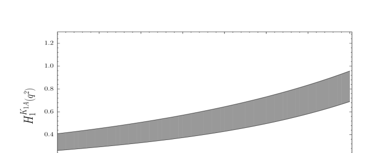
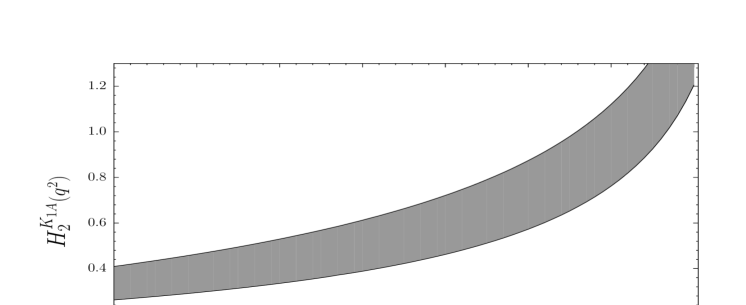
In Figs. (1)–(3) we present the fits of the series expansion
parametrization to LCSR results for the helicity amplitudes H 0 ( q 2 ) subscript 𝐻 0 superscript 𝑞 2 H_{0}(q^{2}) H 1 ( q 2 ) subscript 𝐻 1 superscript 𝑞 2 H_{1}(q^{2}) H 2 ( q 2 ) subscript 𝐻 2 superscript 𝑞 2 H_{2}(q^{2}) b 𝑏 b s 𝑠 s M 2 superscript 𝑀 2 M^{2} s 0 subscript 𝑠 0 s_{0}
In Table 1 we present the values of the coefficients β k ( 0 ) K 1 A superscript subscript 𝛽 𝑘 0 subscript 𝐾 1 𝐴 \beta_{k}^{(0)K_{1A}} β k ( 1 ) K 1 A superscript subscript 𝛽 𝑘 1 subscript 𝐾 1 𝐴 \beta_{k}^{(1)K_{1A}} ( k = 0 , 1 ) 𝑘 0 1
(k=0,1) H 0 ( q 2 ) subscript 𝐻 0 superscript 𝑞 2 H_{0}(q^{2}) H 1 ( q 2 ) subscript 𝐻 1 superscript 𝑞 2 H_{1}(q^{2}) H 2 ( q 2 ) subscript 𝐻 2 superscript 𝑞 2 H_{2}(q^{2}) ∑ k = 0 1 ( β k K 1 A ) 2 superscript subscript 𝑘 0 1 superscript superscript subscript 𝛽 𝑘 subscript 𝐾 1 𝐴 2 \sum_{k=0}^{1}{(\beta_{k}^{K_{1A}})^{2}} 45 z 𝑧 z β k subscript 𝛽 𝑘 \beta_{k} N = 2 𝑁 2 N=2 [19 ] ).
β 0 K 1 A β 1 K 1 A ∑ k = 0 1 ( β k K 1 A ) 2 H 0 3.7 × 10 − 5 − 1.3 × 10 − 3 1.7 × 10 − 6 H 1 8.4 × 10 − 5 − 3.0 × 10 − 3 9.0 × 10 − 6 H 2 2.1 × 10 − 5 − 6.4 × 10 − 4 4.1 × 10 − 7 missing-subexpression missing-subexpression missing-subexpression missing-subexpression missing-subexpression missing-subexpression missing-subexpression missing-subexpression missing-subexpression superscript subscript 𝛽 0 subscript 𝐾 1 𝐴 superscript subscript 𝛽 1 subscript 𝐾 1 𝐴 superscript subscript 𝑘 0 1 superscript superscript subscript 𝛽 𝑘 subscript 𝐾 1 𝐴 2 missing-subexpression missing-subexpression missing-subexpression missing-subexpression missing-subexpression missing-subexpression missing-subexpression missing-subexpression subscript 𝐻 0 3.7 superscript 10 5 1.3 superscript 10 3 1.7 superscript 10 6 subscript 𝐻 1 8.4 superscript 10 5 3.0 superscript 10 3 9.0 superscript 10 6 subscript 𝐻 2 2.1 superscript 10 5 6.4 superscript 10 4 4.1 superscript 10 7 missing-subexpression missing-subexpression missing-subexpression missing-subexpression \begin{array}[]{|l|c|c|c|}\hline\cr\hline\cr&\beta_{0}^{K_{1A}}&\beta_{1}^{K_{1A}}&\sum_{k=0}^{1}{(\beta_{k}^{K_{1A}})^{2}}\\
\hline\cr\hline\cr H_{0}&3.7\times 10^{-5}&-1.3\times 10^{-3}&1.7\times 10^{-6}\\
H_{1}&8.4\times 10^{-5}&-3.0\times 10^{-3}&9.0\times 10^{-6}\\
H_{2}&2.1\times 10^{-5}&-6.4\times 10^{-4}&4.1\times 10^{-7}\\
\hline\cr\hline\cr\end{array}
Table 1: The values of the coefficients β k K 1 A superscript subscript 𝛽 𝑘 subscript 𝐾 1 𝐴 \beta_{k}^{K_{1A}} H 0 ( q 2 ) subscript 𝐻 0 superscript 𝑞 2 H_{0}(q^{2}) H 1 ( q 2 ) subscript 𝐻 1 superscript 𝑞 2 H_{1}(q^{2}) H 2 ( q 2 ) subscript 𝐻 2 superscript 𝑞 2 H_{2}(q^{2})
Our final remark is as follows: As has already been noted, in the numerical
calculations we use f B = 210 ± 19 M e V subscript 𝑓 𝐵 plus-or-minus 210 19 𝑀 𝑒 𝑉 f_{B}=210\pm 19~{}MeV f B = 145 M e V subscript 𝑓 𝐵 145 𝑀 𝑒 𝑉 f_{B}=145~{}MeV [20 ] had been used the
values of all form factors presented in this work increase by a factor 1.4.
In summary, we calculate the tensor form factors of B 𝐵 B P 𝑃 P 𝒪 ( α s ) 𝒪 subscript 𝛼 𝑠 {\cal O}(\alpha_{s})
Distribution amplitudes
The two–parton chiral–even LCDAs are given by
⟨ K 1 ( p , λ ) | s ¯ ( x ) γ μ γ 5 ψ ( 0 ) | 0 ⟩ quantum-operator-product subscript 𝐾 1 𝑝 𝜆 ¯ 𝑠 𝑥 subscript 𝛾 𝜇 subscript 𝛾 5 𝜓 0 0 \displaystyle\langle K_{1}(p,\lambda)|\bar{s}(x)\gamma_{\mu}\gamma_{5}\psi(0)|0\rangle = \displaystyle= i f K 1 m K 1 ∫ 0 1 d u e i u p x { p μ ε ( λ ) ∗ x p x ϕ ∥ ( u ) \displaystyle if_{K_{1}}m_{K_{1}}\,\int_{0}^{1}du\,e^{iu\,px}\Bigg{\{}p_{\mu}\,\frac{\varepsilon^{(\lambda)*}x}{px}\,\phi_{\parallel}(u) (A.1)
+ ( ε μ ( λ ) ∗ − p μ ε ( λ ) ∗ x p x ) g ⟂ ( a ) ( u ) − 1 2 x μ ϵ ∗ ( λ ) x ( p x ) 2 m K 1 2 g ¯ 3 ( u ) superscript subscript 𝜀 𝜇 𝜆
subscript 𝑝 𝜇 superscript 𝜀 𝜆
𝑥 𝑝 𝑥 superscript subscript 𝑔 perpendicular-to 𝑎 𝑢 1 2 subscript 𝑥 𝜇 superscript italic-ϵ absent 𝜆 𝑥 superscript 𝑝 𝑥 2 superscript subscript 𝑚 subscript 𝐾 1 2 subscript ¯ 𝑔 3 𝑢 \displaystyle+\left(\varepsilon_{\mu}^{(\lambda)*}-p_{\mu}\frac{\varepsilon^{(\lambda)*}x}{p\,x}\right)\,g_{\perp}^{(a)}(u)-\frac{1}{2}x_{\mu}\frac{\epsilon^{*(\lambda)}x}{(px)^{2}}m_{K_{1}}^{2}\bar{g}_{3}(u)
+ 𝒪 ( x 2 ) } , \displaystyle+{\cal O}(x^{2})\Bigg{\}}~{},
⟨ K 1 ( p , λ ) | s ¯ ( x ) γ μ ψ ( 0 ) | 0 ⟩ quantum-operator-product subscript 𝐾 1 𝑝 𝜆 ¯ 𝑠 𝑥 subscript 𝛾 𝜇 𝜓 0 0 \displaystyle\langle K_{1}(p,\lambda)|\bar{s}(x)\gamma_{\mu}\psi(0)|0\rangle = \displaystyle= − i f K 1 m K 1 ϵ μ ν ρ σ ε ( λ ) ∗ ν p ρ x σ ∫ 0 1 𝑑 u e i u p x ( g ⟂ ( v ) ( u ) 4 + 𝒪 ( x 2 ) ) , 𝑖 subscript 𝑓 subscript 𝐾 1 subscript 𝑚 subscript 𝐾 1 subscript italic-ϵ 𝜇 𝜈 𝜌 𝜎 superscript 𝜀 𝜆 𝜈 superscript 𝑝 𝜌 superscript 𝑥 𝜎 superscript subscript 0 1 differential-d 𝑢 superscript 𝑒 𝑖 𝑢 𝑝 𝑥 superscript subscript 𝑔 perpendicular-to 𝑣 𝑢 4 𝒪 superscript 𝑥 2 \displaystyle-if_{K_{1}}m_{K_{1}}\,\epsilon_{\mu\nu\rho\sigma}\,\varepsilon^{(\lambda)*\nu}p^{\rho}x^{\sigma}\,\int_{0}^{1}du\,e^{iu\,px}\,\Bigg{(}\frac{g_{\perp}^{(v)}(u)}{4}+{\cal O}(x^{2})\Bigg{)}~{},
where ψ ≡ u ( or d ) 𝜓 𝑢 or 𝑑 \psi\equiv u({\rm or}\ d) x 2 ≠ 0 superscript 𝑥 2 0 x^{2}\not=0 u 𝑢 u s 𝑠 s K 1 A ( B ) subscript 𝐾 1 𝐴 𝐵 K_{1A(B)}
⟨ K 1 ( p , λ ) | s ¯ ( x ) σ μ ν γ 5 ψ ( 0 ) | 0 ⟩ = f K 1 ⟂ ∫ 0 1 d u e i u p x { ( ε μ ( λ ) ∗ p ν − ε ν ( λ ) ∗ p μ ) ϕ ⟂ ( u ) \displaystyle\langle K_{1}(p,\lambda)|\bar{s}(x)\sigma_{\mu\nu}\gamma_{5}\psi(0)|0\rangle=f_{K_{1}}^{\perp}\,\int_{0}^{1}du\,e^{iu\,px}\,\Bigg{\{}(\varepsilon^{(\lambda)*}_{\mu}p_{\nu}-\varepsilon_{\nu}^{(\lambda)*}p_{\mu})\phi_{\perp}(u)
+ m K 1 2 ε ( λ ) ∗ x ( p x ) 2 ( p μ x ν − p ν x μ ) h ¯ ∥ ( t ) ( u ) superscript subscript 𝑚 subscript 𝐾 1 2 superscript 𝜀 𝜆
𝑥 superscript 𝑝 𝑥 2 subscript 𝑝 𝜇 subscript 𝑥 𝜈 subscript 𝑝 𝜈 subscript 𝑥 𝜇 superscript subscript ¯ ℎ parallel-to 𝑡 𝑢 \displaystyle\hskip 142.26378pt+\,\frac{m_{K_{1}}^{2}\,\varepsilon^{(\lambda)*}x}{(px)^{2}}\,(p_{\mu}x_{\nu}-p_{\nu}x_{\mu})\,\bar{h}_{\parallel}^{(t)}(u)
+ 1 2 ( ε μ ∗ ( λ ) x ν − ε ν ∗ ( λ ) x μ ) m K 1 2 p x h ¯ 3 ( u ) + 𝒪 ( x 2 ) } , \displaystyle\hskip 142.26378pt+\frac{1}{2}(\varepsilon^{*(\lambda)}_{\mu}x_{\nu}-\varepsilon^{*(\lambda)}_{\nu}x_{\mu})\frac{m_{K_{1}}^{2}}{px}\bar{h}_{3}(u)+{\cal O}(x^{2})\Bigg{\}}~{}, (A.3)
⟨ K 1 ( p , λ ) | s ¯ ( x ) γ 5 ψ ( 0 ) | 0 ⟩ = f K 1 ⟂ m K 1 2 ( ε ∗ ( λ ) x ) ∫ 0 1 𝑑 u e i u p x ( h ∥ ( p ) ( u ) 2 + 𝒪 ( x 2 ) ) , quantum-operator-product subscript 𝐾 1 𝑝 𝜆 ¯ 𝑠 𝑥 subscript 𝛾 5 𝜓 0 0 superscript subscript 𝑓 subscript 𝐾 1 perpendicular-to superscript subscript 𝑚 subscript 𝐾 1 2 superscript 𝜀 absent 𝜆 𝑥 superscript subscript 0 1 differential-d 𝑢 superscript 𝑒 𝑖 𝑢 𝑝 𝑥 superscript subscript ℎ parallel-to 𝑝 𝑢 2 𝒪 superscript 𝑥 2 \displaystyle\langle K_{1}(p,\lambda)|\bar{s}(x)\gamma_{5}\psi(0)|0\rangle=f_{K_{1}}^{\perp}m_{K_{1}}^{2}(\varepsilon^{*(\lambda)}x)\,\int_{0}^{1}du\,e^{iu\,px}\,\Bigg{(}\frac{h_{\parallel}^{(p)}(u)}{2}+{\cal O}(x^{2})\Bigg{)}~{}, (A.4)
where the functions g ¯ 3 ( u ) subscript ¯ 𝑔 3 𝑢 \bar{g}_{3}(u) h ¯ ∥ ( t ) superscript subscript ¯ ℎ parallel-to 𝑡 \bar{h}_{\parallel}^{(t)} h ¯ 3 ( u ) subscript ¯ ℎ 3 𝑢 \bar{h}_{3}(u) 2 G 𝐺 G ϕ ∥ , g ⟂ ( a ) subscript italic-ϕ parallel-to superscript subscript 𝑔 perpendicular-to 𝑎
\phi_{\parallel},g_{\perp}^{(a)} g ⟂ ( v ) superscript subscript 𝑔 perpendicular-to 𝑣 g_{\perp}^{(v)} g 3 subscript 𝑔 3 g_{3} u → 1 − u → 𝑢 1 𝑢 u\to 1-u 1 3 P 1 superscript 1 3 subscript 𝑃 1 1^{3}P_{1} 1 1 P 1 superscript 1 1 subscript 𝑃 1 1^{1}P_{1} ϕ ⟂ , h ∥ ( t ) subscript italic-ϕ perpendicular-to superscript subscript ℎ parallel-to 𝑡
\phi_{\perp},h_{\parallel}^{(t)} h ∥ ( p ) superscript subscript ℎ parallel-to 𝑝 h_{\parallel}^{(p)} h 3 subscript ℎ 3 h_{3} [14 ] ,
∫ 0 1 𝑑 u ϕ ∥ ( u ) = ∫ 0 1 𝑑 u g ⟂ ( a ) ( u ) = ∫ 0 1 𝑑 u g ⟂ ( v ) ( u ) = 1 , superscript subscript 0 1 differential-d 𝑢 subscript italic-ϕ parallel-to 𝑢 superscript subscript 0 1 differential-d 𝑢 superscript subscript 𝑔 perpendicular-to 𝑎 𝑢 superscript subscript 0 1 differential-d 𝑢 superscript subscript 𝑔 perpendicular-to 𝑣 𝑢 1 \displaystyle\int_{0}^{1}du\phi_{\parallel}(u)=\int_{0}^{1}dug_{\perp}^{(a)}(u)=\int_{0}^{1}dug_{\perp}^{(v)}(u)=1,
∫ 0 1 𝑑 u ϕ ⟂ ( u ) = ∫ 0 1 𝑑 u h ∥ ( t ) ( u ) = a 0 ⟂ , ∫ 0 1 𝑑 u h ∥ ( p ) ( u ) = a 0 ⟂ + δ − , formulae-sequence superscript subscript 0 1 differential-d 𝑢 subscript italic-ϕ perpendicular-to 𝑢 superscript subscript 0 1 differential-d 𝑢 superscript subscript ℎ parallel-to 𝑡 𝑢 superscript subscript 𝑎 0 perpendicular-to superscript subscript 0 1 differential-d 𝑢 superscript subscript ℎ parallel-to 𝑝 𝑢 superscript subscript 𝑎 0 perpendicular-to subscript 𝛿 \displaystyle\int_{0}^{1}du\phi_{\perp}(u)=\int_{0}^{1}duh_{\parallel}^{(t)}(u)=a_{0}^{\perp},\quad\int_{0}^{1}duh_{\parallel}^{(p)}(u)=a_{0}^{\perp}+\delta_{-}~{}, (A.5)
for K 1 A subscript 𝐾 1 𝐴 K_{1A}
∫ 0 1 𝑑 u ϕ ∥ ( u ) = ∫ 0 1 𝑑 u g ⟂ ( a ) ( u ) = a 0 ∥ , ∫ 0 1 𝑑 u g ⟂ ( v ) ( u ) = a 0 ∥ + δ ~ − , formulae-sequence superscript subscript 0 1 differential-d 𝑢 subscript italic-ϕ parallel-to 𝑢 superscript subscript 0 1 differential-d 𝑢 superscript subscript 𝑔 perpendicular-to 𝑎 𝑢 superscript subscript 𝑎 0 parallel-to superscript subscript 0 1 differential-d 𝑢 superscript subscript 𝑔 perpendicular-to 𝑣 𝑢 superscript subscript 𝑎 0 parallel-to subscript ~ 𝛿 \displaystyle\int_{0}^{1}du\phi_{\parallel}(u)=\int_{0}^{1}dug_{\perp}^{(a)}(u)=a_{0}^{\parallel},\quad\int_{0}^{1}dug_{\perp}^{(v)}(u)=a_{0}^{\parallel}+\tilde{\delta}_{-}~{},
∫ 0 1 𝑑 u ϕ ⟂ ( u ) = ∫ 0 1 𝑑 u h ∥ ( t ) ( u ) = ∫ 0 1 𝑑 u h ∥ ( p ) ( u ) = 1 , superscript subscript 0 1 differential-d 𝑢 subscript italic-ϕ perpendicular-to 𝑢 superscript subscript 0 1 differential-d 𝑢 superscript subscript ℎ parallel-to 𝑡 𝑢 superscript subscript 0 1 differential-d 𝑢 superscript subscript ℎ parallel-to 𝑝 𝑢 1 \displaystyle\int_{0}^{1}du\phi_{\perp}(u)=\int_{0}^{1}duh_{\parallel}^{(t)}(u)=\int_{0}^{1}duh_{\parallel}^{(p)}(u)=1, (A.6)
for K 1 B subscript 𝐾 1 𝐵 K_{1B}
δ ~ − = − f K 1 f K 1 ⟂ m s m K 1 , δ ~ − = − f K 1 ⟂ f K 1 m s m K 1 , formulae-sequence subscript ~ 𝛿 subscript 𝑓 subscript 𝐾 1 superscript subscript 𝑓 subscript 𝐾 1 perpendicular-to subscript 𝑚 𝑠 subscript 𝑚 subscript 𝐾 1 subscript ~ 𝛿 superscript subscript 𝑓 subscript 𝐾 1 perpendicular-to subscript 𝑓 subscript 𝐾 1 subscript 𝑚 𝑠 subscript 𝑚 subscript 𝐾 1 \widetilde{\delta}_{-}=-{f_{K_{1}}\over f_{K_{1}}^{\perp}}{m_{s}\over m_{K_{1}}}~{},\qquad\widetilde{\delta}_{-}=-{f_{K_{1}}^{\perp}\over f_{K_{1}}}{m_{s}\over m_{K_{1}}}~{}, (A.7)
and a 0 ∥ , ⟂ a_{0}^{\parallel,\perp}
⟨ K 1 A ( p , λ ) | s ¯ ( 0 ) σ μ ν γ 5 ψ ( 0 ) | 0 ⟩ = f K 1 A a 0 ⟂ , K 1 A ( ε μ ( λ ) ∗ p ν − ε ν ( λ ) ∗ p μ ) , quantum-operator-product subscript 𝐾 1 𝐴 𝑝 𝜆 ¯ 𝑠 0 subscript 𝜎 𝜇 𝜈 subscript 𝛾 5 𝜓 0 0 subscript 𝑓 subscript 𝐾 1 𝐴 superscript subscript 𝑎 0 perpendicular-to subscript 𝐾 1 𝐴
subscript superscript 𝜀 𝜆
𝜇 subscript 𝑝 𝜈 superscript subscript 𝜀 𝜈 𝜆
subscript 𝑝 𝜇 \displaystyle\langle K_{1A}(p,\lambda)|\bar{s}(0)\sigma_{\mu\nu}\gamma_{5}\psi(0)|0\rangle=f_{K_{1A}}a_{0}^{\perp,K_{1A}}\,(\varepsilon^{(\lambda)*}_{\mu}p_{\nu}-\varepsilon_{\nu}^{(\lambda)*}p_{\mu})~{}, (A.8)
⟨ K 1 B ( p , λ ) | s ¯ ( 0 ) γ μ γ 5 ψ ( 0 ) | 0 ⟩ = i f K 1 B ⟂ ( 1 GeV ) a 0 ∥ , K 1 B m K 1 B ε μ ( λ ) ∗ , \displaystyle\langle K_{1B}(p,\lambda)|\bar{s}(0)\gamma_{\mu}\gamma_{5}\psi(0)|0\rangle=if_{K_{1B}}^{\perp}(1~{}{\rm GeV})a_{0}^{\parallel,K_{1B}}\,m_{K_{1B}}\,\varepsilon^{(\lambda)*}_{\mu}~{}, (A.9)
with f K 1 A ⟂ = f K 1 A superscript subscript 𝑓 subscript 𝐾 1 𝐴 perpendicular-to subscript 𝑓 subscript 𝐾 1 𝐴 f_{K_{1A}}^{\perp}=f_{K_{1A}} f P 1 1 = f P 1 1 ⟂ ( μ = 1 GeV ) subscript 𝑓 superscript subscript 𝑃 1 1 superscript subscript 𝑓 superscript subscript 𝑃 1 1 perpendicular-to 𝜇 1 GeV f_{{}^{1}\!P_{1}}=f_{{}^{1}\!P_{1}}^{\perp}(\mu=1~{}{\rm GeV}) a 0 ⟂ , K 1 A superscript subscript 𝑎 0 perpendicular-to subscript 𝐾 1 𝐴
a_{0}^{\perp,K_{1A}} a 0 ∥ , K 1 B a_{0}^{\parallel,K_{1B}}
We use the twist–2 distributions
[14 ]
ϕ ∥ ( u ) subscript italic-ϕ parallel-to 𝑢 \displaystyle\phi_{\parallel}(u) = \displaystyle= 6 u u ¯ [ 1 + 3 a 1 ∥ ξ + a 2 ∥ 3 2 ( 5 ξ 2 − 1 ) ] , 6 𝑢 ¯ 𝑢 delimited-[] 1 3 superscript subscript 𝑎 1 parallel-to 𝜉 superscript subscript 𝑎 2 parallel-to 3 2 5 superscript 𝜉 2 1 \displaystyle 6u\bar{u}\left[1+3a_{1}^{\parallel}\,\xi+a_{2}^{\parallel}\,\frac{3}{2}(5\xi^{2}-1)\right]~{}, (A.10)
ϕ ⟂ ( u ) subscript italic-ϕ perpendicular-to 𝑢 \displaystyle\phi_{\perp}(u) = \displaystyle= 6 u u ¯ [ a 0 ⟂ + 3 a 1 ⟂ ξ + a 2 ⟂ 3 2 ( 5 ξ 2 − 1 ) ] , 6 𝑢 ¯ 𝑢 delimited-[] superscript subscript 𝑎 0 perpendicular-to 3 superscript subscript 𝑎 1 perpendicular-to 𝜉 superscript subscript 𝑎 2 perpendicular-to 3 2 5 superscript 𝜉 2 1 \displaystyle 6u\bar{u}\left[a_{0}^{\perp}+3a_{1}^{\perp}\,\xi+a_{2}^{\perp}\,\frac{3}{2}(5\xi^{2}-1)\right]~{}, (A.11)
for the K 1 A subscript 𝐾 1 𝐴 K_{1A}
ϕ ∥ ( u ) subscript italic-ϕ parallel-to 𝑢 \displaystyle\phi_{\parallel}(u) = \displaystyle= 6 u u ¯ [ a 0 ∥ + 3 a 1 ∥ ξ + a 2 ∥ 3 2 ( 5 ξ 2 − 1 ) ] , 6 𝑢 ¯ 𝑢 delimited-[] superscript subscript 𝑎 0 parallel-to 3 superscript subscript 𝑎 1 parallel-to 𝜉 superscript subscript 𝑎 2 parallel-to 3 2 5 superscript 𝜉 2 1 \displaystyle 6u\bar{u}\left[a_{0}^{\parallel}+3a_{1}^{\parallel}\,\xi+a_{2}^{\parallel}\,\frac{3}{2}(5\xi^{2}-1)\right]~{}, (A.12)
ϕ ⟂ ( u ) subscript italic-ϕ perpendicular-to 𝑢 \displaystyle\phi_{\perp}(u) = \displaystyle= 6 u u ¯ [ 1 + 3 a 1 ⟂ ξ + a 2 ⟂ 3 2 ( 5 ξ 2 − 1 ) ] , 6 𝑢 ¯ 𝑢 delimited-[] 1 3 superscript subscript 𝑎 1 perpendicular-to 𝜉 superscript subscript 𝑎 2 perpendicular-to 3 2 5 superscript 𝜉 2 1 \displaystyle 6u\bar{u}\left[1+3a_{1}^{\perp}\,\xi+a_{2}^{\perp}\,\frac{3}{2}(5\xi^{2}-1)\right]~{}, (A.13)
for the K 1 B subscript 𝐾 1 𝐵 K_{1B} ξ = 2 u − 1 𝜉 2 𝑢 1 \xi=2u-1 9 / 2 9 2 9/2
𝒜 𝒜 \displaystyle{\cal A} = \displaystyle= 5040 ( α 1 − α 2 ) α 1 α 2 α 3 2 + 360 α 1 α 2 α 3 2 [ λ K 1 A A + σ K 1 A A 1 2 ( 7 α 3 − 3 ) ] , 5040 subscript 𝛼 1 subscript 𝛼 2 subscript 𝛼 1 subscript 𝛼 2 superscript subscript 𝛼 3 2 360 subscript 𝛼 1 subscript 𝛼 2 superscript subscript 𝛼 3 2 delimited-[] subscript superscript 𝜆 𝐴 subscript 𝐾 1 𝐴 subscript superscript 𝜎 𝐴 subscript 𝐾 1 𝐴 1 2 7 subscript 𝛼 3 3 \displaystyle 5040(\alpha_{1}-\alpha_{2})\alpha_{1}\alpha_{2}\alpha_{3}^{2}+360\alpha_{1}\alpha_{2}\alpha_{3}^{2}\Big{[}\lambda^{A}_{K_{1A}}+\sigma^{A}_{K_{1A}}\frac{1}{2}(7\alpha_{3}-3)\Big{]}~{}, (A.14)
𝒱 𝒱 \displaystyle{\cal V} = \displaystyle= 360 α 1 α 2 α 3 2 [ 1 + ω K 1 A V 1 2 ( 7 α 3 − 3 ) ] + 5040 ( α 1 − α 2 ) α 1 α 2 α 3 2 σ K 1 A V , 360 subscript 𝛼 1 subscript 𝛼 2 superscript subscript 𝛼 3 2 delimited-[] 1 subscript superscript 𝜔 𝑉 subscript 𝐾 1 𝐴 1 2 7 subscript 𝛼 3 3 5040 subscript 𝛼 1 subscript 𝛼 2 subscript 𝛼 1 subscript 𝛼 2 superscript subscript 𝛼 3 2 subscript superscript 𝜎 𝑉 subscript 𝐾 1 𝐴 \displaystyle 360\alpha_{1}\alpha_{2}\alpha_{3}^{2}\Big{[}1+\omega^{V}_{K_{1A}}\frac{1}{2}(7\alpha_{3}-3)\Big{]}+5040(\alpha_{1}-\alpha_{2})\alpha_{1}\alpha_{2}\alpha_{3}^{2}\sigma^{V}_{K_{1A}}~{}, (A.15)
for the K 1 A subscript 𝐾 1 𝐴 K_{1A}
𝒜 𝒜 \displaystyle{\cal A} = \displaystyle= 360 α 1 α 2 α 3 2 [ 1 + ω K 1 B A 1 2 ( 7 α 3 − 3 ) ] + 5040 ( α 1 − α 2 ) α 1 α 2 α 3 2 σ K 1 B A , 360 subscript 𝛼 1 subscript 𝛼 2 superscript subscript 𝛼 3 2 delimited-[] 1 subscript superscript 𝜔 𝐴 subscript 𝐾 1 𝐵 1 2 7 subscript 𝛼 3 3 5040 subscript 𝛼 1 subscript 𝛼 2 subscript 𝛼 1 subscript 𝛼 2 superscript subscript 𝛼 3 2 subscript superscript 𝜎 𝐴 subscript 𝐾 1 𝐵 \displaystyle 360\alpha_{1}\alpha_{2}\alpha_{3}^{2}\Big{[}1+\omega^{A}_{K_{1B}}\frac{1}{2}(7\alpha_{3}-3)\Big{]}+5040(\alpha_{1}-\alpha_{2})\alpha_{1}\alpha_{2}\alpha_{3}^{2}\sigma^{A}_{K_{1B}}~{}, (A.16)
𝒱 𝒱 \displaystyle{\cal V} = \displaystyle= 5040 ( α 1 − α 2 ) α 1 α 2 α 3 2 + 360 α 1 α 2 α 3 2 [ λ K 1 B V + σ K 1 B V 1 2 ( 7 α 3 − 3 ) ] , 5040 subscript 𝛼 1 subscript 𝛼 2 subscript 𝛼 1 subscript 𝛼 2 superscript subscript 𝛼 3 2 360 subscript 𝛼 1 subscript 𝛼 2 superscript subscript 𝛼 3 2 delimited-[] subscript superscript 𝜆 𝑉 subscript 𝐾 1 𝐵 subscript superscript 𝜎 𝑉 subscript 𝐾 1 𝐵 1 2 7 subscript 𝛼 3 3 \displaystyle 5040(\alpha_{1}-\alpha_{2})\alpha_{1}\alpha_{2}\alpha_{3}^{2}+360\alpha_{1}\alpha_{2}\alpha_{3}^{2}\Big{[}\lambda^{V}_{K_{1B}}+\sigma^{V}_{K_{1B}}\frac{1}{2}(7\alpha_{3}-3)\Big{]}~{}, (A.17)
for the K 1 B subscript 𝐾 1 𝐵 K_{1B} λ 𝜆 \lambda ω 𝜔 \omega σ 𝜎 \sigma λ 𝜆 \lambda σ 𝜎 \sigma
For the relevant two–parton twist–3 chiral–even LCDAs, we take the approximate
expressions up to conformal spin 9 / 2 9 2 9/2 m s subscript 𝑚 𝑠 m_{s} [14 ] :
g ⟂ ( a ) ( u ) superscript subscript 𝑔 perpendicular-to 𝑎 𝑢 \displaystyle g_{\perp}^{(a)}(u) = \displaystyle= 3 4 ( 1 + ξ 2 ) + 3 2 a 1 ∥ ξ 3 + ( 3 7 a 2 ∥ + 5 ζ 3 , K 1 A V ) ( 3 ξ 2 − 1 ) 3 4 1 superscript 𝜉 2 3 2 superscript subscript 𝑎 1 parallel-to superscript 𝜉 3 3 7 superscript subscript 𝑎 2 parallel-to 5 superscript subscript 𝜁 3 subscript 𝐾 1 𝐴
𝑉 3 superscript 𝜉 2 1 \displaystyle\frac{3}{4}(1+\xi^{2})+\frac{3}{2}\,a_{1}^{\parallel}\,\xi^{3}+\left(\frac{3}{7}\,a_{2}^{\parallel}+5\zeta_{3,K_{1A}}^{V}\right)\left(3\xi^{2}-1\right) (A.18)
+ ( 9 112 a 2 ∥ + 105 16 ζ 3 , K 1 A A − 15 64 ζ 3 , K 1 A V ω K 1 A V ) ( 35 ξ 4 − 30 ξ 2 + 3 ) 9 112 superscript subscript 𝑎 2 parallel-to 105 16 superscript subscript 𝜁 3 subscript 𝐾 1 𝐴
𝐴 15 64 superscript subscript 𝜁 3 subscript 𝐾 1 𝐴
𝑉 superscript subscript 𝜔 subscript 𝐾 1 𝐴 𝑉 35 superscript 𝜉 4 30 superscript 𝜉 2 3 \displaystyle{}+\left(\frac{9}{112}\,a_{2}^{\parallel}+\frac{105}{16}\,\zeta_{3,K_{1A}}^{A}-\frac{15}{64}\,\zeta_{3,K_{1A}}^{V}\omega_{K_{1A}}^{V}\right)\left(35\xi^{4}-30\xi^{2}+3\right)
+ 5 [ 21 4 ζ 3 , K 1 A V σ K 1 A V + ζ 3 , K 1 A A ( λ K 1 A A − 3 16 σ K 1 A A ) ] ξ ( 5 ξ 2 − 3 ) 5 delimited-[] 21 4 superscript subscript 𝜁 3 subscript 𝐾 1 𝐴
𝑉 superscript subscript 𝜎 subscript 𝐾 1 𝐴 𝑉 superscript subscript 𝜁 3 subscript 𝐾 1 𝐴
𝐴 superscript subscript 𝜆 subscript 𝐾 1 𝐴 𝐴 3 16 superscript subscript 𝜎 subscript 𝐾 1 𝐴 𝐴 𝜉 5 superscript 𝜉 2 3 \displaystyle+5\Bigg{[}\frac{21}{4}\zeta_{3,K_{1A}}^{V}\sigma_{K_{1A}}^{V}+\zeta_{3,K_{1A}}^{A}\bigg{(}\lambda_{K_{1A}}^{A}-\frac{3}{16}\sigma_{K_{1A}}^{A}\Bigg{)}\Bigg{]}\xi(5\xi^{2}-3)
− 9 2 a 1 ⟂ δ ~ + ( 3 2 + 3 2 ξ 2 + ln u + ln u ¯ ) − 9 2 a 1 ⟂ δ ~ − ( 3 ξ + ln u ¯ − ln u ) , 9 2 superscript subscript 𝑎 1 perpendicular-to subscript ~ 𝛿 3 2 3 2 superscript 𝜉 2 𝑢 ¯ 𝑢 9 2 superscript subscript 𝑎 1 perpendicular-to subscript ~ 𝛿 3 𝜉 ¯ 𝑢 𝑢 \displaystyle{}-\frac{9}{2}{a}_{1}^{\perp}\,\widetilde{\delta}_{+}\,\left(\frac{3}{2}+\frac{3}{2}\xi^{2}+\ln u+\ln\bar{u}\right)-\frac{9}{2}{a}_{1}^{\perp}\,\widetilde{\delta}_{-}\,(3\xi+\ln\bar{u}-\ln u)~{},
g ⟂ ( v ) ( u ) superscript subscript 𝑔 perpendicular-to 𝑣 𝑢 \displaystyle g_{\perp}^{(v)}(u) = \displaystyle= 6 u u ¯ { 1 + ( a 1 ∥ + 20 3 ζ 3 , K 1 A A λ K 1 A A ) ξ \displaystyle 6u\bar{u}\Bigg{\{}1+\Bigg{(}a_{1}^{\parallel}+\frac{20}{3}\zeta_{3,K_{1A}}^{A}\lambda_{K_{1A}}^{A}\Bigg{)}\xi (A.19)
+ [ 1 4 a 2 ∥ + 5 3 ζ 3 , K 1 A V ( 1 − 3 16 ω K 1 A V ) + 35 4 ζ 3 , K 1 A A ] ( 5 ξ 2 − 1 ) delimited-[] 1 4 superscript subscript 𝑎 2 parallel-to 5 3 subscript superscript 𝜁 𝑉 3 subscript 𝐾 1 𝐴
1 3 16 subscript superscript 𝜔 𝑉 subscript 𝐾 1 𝐴 35 4 subscript superscript 𝜁 𝐴 3 subscript 𝐾 1 𝐴
5 superscript 𝜉 2 1 \displaystyle+\Bigg{[}\frac{1}{4}a_{2}^{\parallel}+\frac{5}{3}\,\zeta^{V}_{3,K_{1A}}\left(1-\frac{3}{16}\,\omega^{V}_{K_{1A}}\right)+\frac{35}{4}\zeta^{A}_{3,K_{1A}}\Bigg{]}(5\xi^{2}-1)
+ 35 4 ( ζ 3 , K 1 A V σ K 1 A V − 1 28 ζ 3 , K 1 A A σ K 1 A A ) ξ ( 7 ξ 2 − 3 ) } \displaystyle+\frac{35}{4}\Bigg{(}\zeta_{3,K_{1A}}^{V}\sigma_{K_{1A}}^{V}-\frac{1}{28}\zeta_{3,K_{1A}}^{A}\sigma_{K_{1A}}^{A}\Bigg{)}\xi(7\xi^{2}-3)\Bigg{\}}
− 18 a 1 ⟂ δ ~ + ( 3 u u ¯ + u ¯ ln u ¯ + u ln u ) − 18 a 1 ⟂ δ ~ − ( u u ¯ ξ + u ¯ ln u ¯ − u ln u ) , 18 superscript subscript 𝑎 1 perpendicular-to subscript ~ 𝛿 3 𝑢 ¯ 𝑢 ¯ 𝑢 ¯ 𝑢 𝑢 𝑢 18 superscript subscript 𝑎 1 perpendicular-to subscript ~ 𝛿 𝑢 ¯ 𝑢 𝜉 ¯ 𝑢 ¯ 𝑢 𝑢 𝑢 \displaystyle{}-18\,a_{1}^{\perp}\widetilde{\delta}_{+}\,(3u\bar{u}+\bar{u}\ln\bar{u}+u\ln u)-18\,a_{1}^{\perp}\widetilde{\delta}_{-}\,(u\bar{u}\xi+\bar{u}\ln\bar{u}-u\ln u)~{},
for the K 1 A subscript 𝐾 1 𝐴 K_{1A}
g ⟂ ( a ) ( u ) superscript subscript 𝑔 perpendicular-to 𝑎 𝑢 \displaystyle g_{\perp}^{(a)}(u) = \displaystyle= 3 4 a 0 ∥ ( 1 + ξ 2 ) + 3 2 a 1 ∥ ξ 3 + 5 [ 21 4 ζ 3 , K 1 B V + ζ 3 , K 1 B A ( 1 − 3 16 ω K 1 B A ) ] ξ ( 5 ξ 2 − 3 ) 3 4 superscript subscript 𝑎 0 parallel-to 1 superscript 𝜉 2 3 2 superscript subscript 𝑎 1 parallel-to superscript 𝜉 3 5 delimited-[] 21 4 superscript subscript 𝜁 3 subscript 𝐾 1 𝐵
𝑉 superscript subscript 𝜁 3 subscript 𝐾 1 𝐵
𝐴 1 3 16 superscript subscript 𝜔 subscript 𝐾 1 𝐵 𝐴 𝜉 5 superscript 𝜉 2 3 \displaystyle\frac{3}{4}a_{0}^{\parallel}(1+\xi^{2})+\frac{3}{2}\,a_{1}^{\parallel}\,\xi^{3}+5\left[\frac{21}{4}\,\zeta_{3,K_{1B}}^{V}+\zeta_{3,K_{1B}}^{A}\Bigg{(}1-\frac{3}{16}\omega_{K_{1B}}^{A}\Bigg{)}\right]\xi\left(5\xi^{2}-3\right) (A.20)
+ 3 16 a 2 ∥ ( 15 ξ 4 − 6 ξ 2 − 1 ) + 5 ζ 3 , K 1 B V λ K 1 B V ( 3 ξ 2 − 1 ) 3 16 superscript subscript 𝑎 2 parallel-to 15 superscript 𝜉 4 6 superscript 𝜉 2 1 5 subscript superscript 𝜁 𝑉 3 subscript 𝐾 1 𝐵
subscript superscript 𝜆 𝑉 subscript 𝐾 1 𝐵 3 superscript 𝜉 2 1 \displaystyle{}+\frac{3}{16}\,a_{2}^{\parallel}\left(15\xi^{4}-6\xi^{2}-1\right)+5\,\zeta^{V}_{3,K_{1B}}\lambda^{V}_{K_{1B}}\left(3\xi^{2}-1\right)
+ 105 16 ( ζ 3 , K 1 B A σ K 1 B A − 1 28 ζ K 1 B V σ K 1 B V ) ( 35 ξ 4 − 30 ξ 2 + 3 ) 105 16 subscript superscript 𝜁 𝐴 3 subscript 𝐾 1 𝐵
subscript superscript 𝜎 𝐴 subscript 𝐾 1 𝐵 1 28 subscript superscript 𝜁 𝑉 subscript 𝐾 1 𝐵 subscript superscript 𝜎 𝑉 subscript 𝐾 1 𝐵 35 superscript 𝜉 4 30 superscript 𝜉 2 3 \displaystyle{}+\frac{105}{16}\left(\zeta^{A}_{3,K_{1B}}\sigma^{A}_{K_{1B}}-\frac{1}{28}\zeta^{V}_{K_{1B}}\sigma^{V}_{K_{1B}}\right)\left(35\xi^{4}-30\xi^{2}+3\right)
− 15 a 2 ⟂ [ δ ~ + ξ 3 + 1 2 δ ~ − ( 3 ξ 2 − 1 ) ] 15 superscript subscript 𝑎 2 perpendicular-to delimited-[] subscript ~ 𝛿 superscript 𝜉 3 1 2 subscript ~ 𝛿 3 superscript 𝜉 2 1 \displaystyle{}-15{a}_{2}^{\perp}\bigg{[}\widetilde{\delta}_{+}\xi^{3}+\frac{1}{2}\widetilde{\delta}_{-}(3\xi^{2}-1)\bigg{]}
− 3 2 [ δ ~ + ( 2 ξ + ln u ¯ − ln u ) + δ ~ − ( 2 + ln u + ln u ¯ ) ] ( 1 + 6 a 2 ⟂ ) , 3 2 delimited-[] subscript ~ 𝛿 2 𝜉 ¯ 𝑢 𝑢 subscript ~ 𝛿 2 𝑢 ¯ 𝑢 1 6 superscript subscript 𝑎 2 perpendicular-to \displaystyle{}-\frac{3}{2}\,\bigg{[}\widetilde{\delta}_{+}\,(2\xi+\ln\bar{u}-\ln u)+\,\widetilde{\delta}_{-}\,(2+\ln u+\ln\bar{u})\bigg{]}(1+6a_{2}^{\perp})~{},
g ⟂ ( v ) ( u ) superscript subscript 𝑔 perpendicular-to 𝑣 𝑢 \displaystyle g_{\perp}^{(v)}(u) = \displaystyle= 6 u u ¯ { a 0 ∥ + a 1 ∥ ξ + [ 1 4 a 2 ∥ + 5 3 ζ 3 , K 1 B V ( λ K 1 B V − 3 16 σ K 1 B V ) + 35 4 ζ 3 , K 1 B A σ K 1 B A ] ( 5 ξ 2 − 1 ) \displaystyle 6u\bar{u}\Bigg{\{}a_{0}^{\parallel}+a_{1}^{\parallel}\xi+\Bigg{[}\frac{1}{4}a_{2}^{\parallel}+\frac{5}{3}\zeta^{V}_{3,K_{1B}}\Bigg{(}\lambda^{V}_{K_{1B}}-\frac{3}{16}\sigma^{V}_{K_{1B}}\Bigg{)}+\frac{35}{4}\zeta^{A}_{3,K_{1B}}\sigma^{A}_{K_{1B}}\Bigg{]}(5\xi^{2}-1) (A.21)
+ 20 3 ξ [ ζ 3 , K 1 B A + 21 16 ( ζ 3 , K 1 B V − 1 28 ζ 3 , K 1 B A ω K 1 B A ) ( 7 ξ 2 − 3 ) ] 20 3 𝜉 delimited-[] subscript superscript 𝜁 𝐴 3 subscript 𝐾 1 𝐵
21 16 subscript superscript 𝜁 𝑉 3 subscript 𝐾 1 𝐵
1 28 subscript superscript 𝜁 𝐴 3 subscript 𝐾 1 𝐵
subscript superscript 𝜔 𝐴 subscript 𝐾 1 𝐵 7 superscript 𝜉 2 3 \displaystyle{}+\frac{20}{3}\,\xi\left[\zeta^{A}_{3,K_{1B}}+\frac{21}{16}\Bigg{(}\zeta^{V}_{3,K_{1B}}-\frac{1}{28}\,\zeta^{A}_{3,K_{1B}}\omega^{A}_{K_{1B}}\Bigg{)}(7\xi^{2}-3)\right]
− 5 a 2 ⟂ [ 2 δ ~ + ξ + δ ~ − ( 1 + ξ 2 ) ] } \displaystyle{}-5\,a_{2}^{\perp}[2\widetilde{\delta}_{+}\xi+\widetilde{\delta}_{-}(1+\xi^{2})]\Bigg{\}}
− 6 [ δ ~ + ( u ¯ ln u ¯ − u ln u ) + δ ~ − ( 2 u u ¯ + u ¯ ln u ¯ + u ln u ) ] ( 1 + 6 a 2 ⟂ ) , 6 delimited-[] subscript ~ 𝛿 ¯ 𝑢 ¯ 𝑢 𝑢 𝑢 subscript ~ 𝛿 2 𝑢 ¯ 𝑢 ¯ 𝑢 ¯ 𝑢 𝑢 𝑢 1 6 superscript subscript 𝑎 2 perpendicular-to \displaystyle{}-6\bigg{[}\,\widetilde{\delta}_{+}\,(\bar{u}\ln\bar{u}-u\ln u)+\,\widetilde{\delta}_{-}\,(2u\bar{u}+\bar{u}\ln\bar{u}+u\ln u)\bigg{]}(1+6a_{2}^{\perp})~{},
for the K 1 B subscript 𝐾 1 𝐵 K_{1B}
δ ~ ± = ± f K 1 ⟂ f K 1 m s m K 1 , ζ 3 , K 1 V ( A ) = f 3 K 1 V ( A ) f K 1 m K 1 . formulae-sequence subscript ~ 𝛿 plus-or-minus plus-or-minus superscript subscript 𝑓 subscript 𝐾 1 perpendicular-to subscript 𝑓 subscript 𝐾 1 subscript 𝑚 𝑠 subscript 𝑚 subscript 𝐾 1 superscript subscript 𝜁 3 subscript 𝐾 1
𝑉 𝐴 subscript superscript 𝑓 𝑉 𝐴 3 subscript 𝐾 1 subscript 𝑓 subscript 𝐾 1 subscript 𝑚 subscript 𝐾 1 \widetilde{\delta}_{\pm}=\pm{f_{K_{1}}^{\perp}\over f_{K_{1}}}{m_{s}\over m_{K_{1}}}~{},\qquad\zeta_{3,K_{1}}^{V(A)}=\frac{f^{V(A)}_{3K_{1}}}{f_{K_{1}}m_{K_{1}}}~{}. (A.22)
The relevant parameters entering to the expressions of DAs are listed in
Table 3.
Figure 1: The dependence of the helicity amplitude H 0 ( q 2 ) subscript 𝐻 0 superscript 𝑞 2 H_{0}(q^{2}) q 2 superscript 𝑞 2 q^{2} z 𝑧 z B → K 1 A → 𝐵 subscript 𝐾 1 𝐴 B\to K_{1A}
Figure 2: The same as in Fig. (1), but for the helicity amplitude H 1 ( q 2 ) subscript 𝐻 1 superscript 𝑞 2 H_{1}(q^{2})
Figure 3: The same as in Fig. (1), but for the helicity amplitude H 2 ( q 2 ) subscript 𝐻 2 superscript 𝑞 2 H_{2}(q^{2})