Weaving independently generated photons into an arbitrary graph state

Abstract

The controlled Z (CZ) operations acting separately on pairs of qubits are commonly adopted in the schemes of generating graph states, the multi-partite entangled states for the one-way quantum computing. For this purpose, we propose a setup of cascade CZ operation on a whole group of qubits in sequence. The operation of the setup starts with entangling an ancilla photon to the first photon as qubit, and this ancilla automatically moves from one entanglement link to another in assisting the formation of a string in graph states. The generation of some special types of graph states, such as the three-dimensional ones, can be greatly simplified in this approach. The setup presented uses weak nonlinearities, but an implementation using probabilistic linear optics is also possible.

I Introduction

The one-way quantum computing cluster1 ; cluster2 ; cluster3 attracts wide attention for its efficiency and simplicity. Different from the traditional circuit-based quantum computing, it only works with single-qubit measurements on the apriori prepared multi-entangled states called graph states or cluster states. The graph states form an important class of multi-partite entangled states. In addition to the two-dimensional (2D) graph states, three dimensional (3D) graph states have been suggested for fault-tolerant one-way quantum computing 3D . How to efficiently generate these graph states is the main problem in realizing practical one-way quantum computing.

Photons have long coherence time and interact weakly with their environment. Photonic qubits, including the discrete ones (see e.g. Nielsen1 ; Browne ; Gilbert ; dc-c1 ) and the continuous variable (CV) ones (see e.g. cv-1 ; cv-2 ; cv-3 ), are among the first candidates for the one-way quantum computing. Although there have existed numerous proof of principle experiments experiments1 ; experiments2 ; k ; pan1 ; y ; pan2 to demonstrate the generation of graph states of a few photons, these linear optical approaches are not efficient enough for making graph states of many qubits due to their limited success probabilities in basic entangling operations. Deterministic gates employing photonic nonlinearity are necessary for the practical one-way quantum computing. The straightforward way of entangling photonic qubits is to apply deterministic controlled-Z (CZ) gate working with strong photon-photon interaction in nonlinear media. However, in addition to the generic weak interaction between photons and the accompanying decoherence from losses in media, the realization of high-quality photon-photon gates is hindered by physical limitations such as multi-mode effects shap1 ; bana ; multi ; qft . An alternative for realizing deterministic photonic gates is the weak nonlinearity between photons and coherent states with large amplitude Nemoto ; Barrett . So far the schemes based on weak nonlinearity have been proposed for generating 2D graph states of atomic qubits Spiller1 ; Spiller2 ; hors or photonic qubits Spiller3 ; Lin3 . The operations in generating graph states of large number of qubits should be also optimized, so that the demanded resources could be as few as possible hors . This problem is more relevant to graph states of photonic qubits, which should be prepared quickly if given no perfect quantum memory.

To have a clearer picture of the problem, we look at how a graph state is built up from the inputs. Most of theoretical works adopt the link by link entanglement connection between qubits by separate CZ operations. Given weak nonlinearity, each CZ operation requires two entangler or parity gate operations, which consume an ancilla photon, respectively Nemoto . Another approach for speeding up graph state generation is to manufacture a target graph state with the building blocks initially prepared from the elementary qubits. For example, in Lin3 we propose a procedure of generating 2D graph states in this fashion; the box-shaped building blocks are first prepared from qubits with entangler operations together with CZ operations, and then the building blocks are assembled to the target graph state by CZ operations. This approach reduces most of CZ operations to deterministic entangler or parity gate operations. To reduce the total preparation time, however, a considerable number of entanglers should be used to prepare the building blocks simultaneously. This necessitates a trade-off of the preparation times for the preparation resources.

Here we present an architecture of cascade CZ operation to solve the problem. By cascade CZ operation we mean that the CZ operations to entangle qubits into a string are bundled together and performed by a single setup called cascade entangler. Such operation is assisted by only one ancilla photon called spider photon, which moves from one entanglement link to another throughout a cascade CZ operation and acts like a spider weaving qubits into a graph state. With cascade CZ operations, the number of facilities for simultaneous operations in generating a graph state, as well as the corresponding ancilla photon number, could be reduced to that of connected strings in the graph state. Moreover, because of the flexible passage of a spider photon, such setup is able to generate an arbitrary graph state.

The rest of the paper is organized as follows. In Sec. II we provide a detailed description of how cascade entangler works for our purpose. The generation of clusters states is illustrated in Sec. III with examples, where we emphasize the advantage of the approach generating 3D graph states. Finally, in Sec. IV we give more discussion on the core element, cross-Kerr nonlinearity, in our setup, and conclude the paper.

II Cascade entangler and cascade CZ operation

The design of cascade entangler is based on the following decomposition of a general graph state review :

$$|G\rangle =\prod_{(i,j)\in E}CZ_{i,j}|+\rangle^{\otimes V}$$

$$=\prod_{(i,j)\in E_{1}}CZ_{i,j}|+\rangle^{\otimes V_{1}}\cdots\prod_{(i,j)\in E_{n}}CZ_{i,j}|+\rangle^{\otimes V_{n}},$$ (1)

where $|\pm\rangle=\frac{1}{\sqrt{2}}(|0\rangle\pm|1\rangle)$ is a qubit on a vertex in the sets $V_{i}$, and $CZ_{i,j}$ denotes the CZ operation over the link between vertex $i$ and $j$. By the above expression, a general graph state is decomposed into a product of the connected string structures $E_{i}$. Note that the CZ operations in the above equation commute and the decomposition to the products of the different connected strings is not unique. The setup is designed to successively entangle the qubits to the string structures $E_{i}$, and the creation of these strings is assisted by a spider photon. If a graph state is in the shape of a single string $E$ (the number of set $E_{i}$ in Eq. (1) equals to one), the setup will directly generate the graph state by the repeated entangling operations on the input qubits. Given $n$ simultaneous operations to generate the strings $E_{i}$, a graph state could be created in an efficiently way.

We illustrate the operation of a cascade entangler with the following input state involving photons $p$, $r$ and the spider photon $a$ as the ancilla (the qubits are encoded with the polarization modes, $|0\rangle\equiv|H\rangle$, $|1\rangle\equiv|V\rangle$):

$$|\Psi\rangle_{in} =(\left|\psi_{1}\right\rangle\left|0\right\rangle_{p}\left|+\right\rangle_{a}+\left|\psi_{2}\right\rangle\left|1\right\rangle_{p}\left|-\right\rangle_{a})\otimes(|0\rangle_{r}+|1\rangle_{r})$$

$$=\big{(}\left|\psi_{1}\right\rangle\left|00\right\rangle\left|+\right\rangle+\left|\psi_{1}\right\rangle\left|01\right\rangle\left|+\right\rangle+\left|\psi_{2}\right\rangle\left|10\right\rangle\left|-\right\rangle$$

$$+\left|\psi_{2}\right\rangle\left|11\right\rangle\left|-\right\rangle\big{)}_{pra},$$ (2)

where $\left|\psi_{i}\right\rangle$, for $i=1,2$, are the proper unnormalized pure states involving other photons than $p$. Here we assume that the spider photon $a$ has been entangled to the finished piece of a graph state, and photon $r$ will be attached to this piece. The already prepared piece $\left|\psi_{1}\right\rangle\left|0\right\rangle_{p}+\left|\psi_{2}\right\rangle\left|1\right\rangle_{p}$ can be a general graph state, but the spider photon $a$ is always entangled to the neighboring photon in the finished piece (photon $p$, for example) in a specific way, i.e., $|+\rangle_{a}$ ($|-\rangle_{a}$) is guaranteed to be in the same terms with $|0\rangle_{p}$ ($|1\rangle_{p}$); see Eq. (2). The purpose for such choice in cascade CZ operation will be seen below.

Figure 1: (color online) Cascade entangler based on cross-phase modulation between photons and coherent states. The two qubus beams are coupled to the $\left|0\right\rangle$, $\left|1\right\rangle$ of the photons $r$ and $a$ as indicated. The ancilla photon (spider photon) is denoted as $a$. A phase shift $-\theta$ is applied to the qubus beams respectively. The qubus beam is divided and merged by 50:50 beam splitters. The single-qubit operations $\sigma_{x}$ and $\sigma_{z}$ are conditionally implemented according to the detection results of the QND module.

We begin with using two polarization beam splitters (PBS) to divide the photons $r$ and $a$ into two spatial modes, respectively. Then two quantum bus (qubus) beams in the coherent state $\left|\alpha\right\rangle$ are coupled with single photon $r$ and $a$ through the weak cross-Kerr nonlinearities; see Fig. 1 for the coupling pattern. All induced phase shifts from cross-phase modulation (XPM) between coherent and single photon state are assumed to be $\theta$. After that, two phase shifters of $-\theta$ are respectively applied to the qubus beams to obtain the state

$$~{}~{}~{}(\left|\psi_{1}\right\rangle\left|0\right\rangle_{p}\left|0\right\rangle_{r}\left|0\right\rangle_{a}+\left|\psi_{1}\right\rangle\left|0\right\rangle_{p}\left|1\right\rangle_{r}\left|1\right\rangle_{a})\left|\alpha\right\rangle\left|\alpha\right\rangle$$

$$+(\left|\psi_{2}\right\rangle\left|1\right\rangle_{p}\left|0\right\rangle_{r}\left|0\right\rangle_{a}-\left|\psi_{2}\right\rangle\left|1\right\rangle_{p}\left|1\right\rangle_{r}\left|1\right\rangle_{a})\left|\alpha\right\rangle\left|\alpha\right\rangle$$

$$+(\left|\psi_{1}\right\rangle\left|0\right\rangle_{p}-\left|\psi_{2}\right\rangle\left|1\right\rangle_{p})\left|0\right\rangle_{r}\left|1\right\rangle_{a}\left|\alpha e^{-i\theta}\right\rangle\left|\alpha e^{i\theta}\right\rangle$$

$$+(\left|\psi_{1}\right\rangle\left|0\right\rangle_{p}+\left|\psi_{2}\right\rangle\left|1\right\rangle_{p})\left|1\right\rangle_{r}\left|0\right\rangle_{a}\left|\alpha e^{i\theta}\right\rangle\left|\alpha e^{-i\theta}\right\rangle.$$ (3)

Next, one 50:50 beam splitter (BS) performs the transformation $\left|\alpha_{1}\right\rangle\left|\alpha_{2}\right\rangle\rightarrow\left|\frac{\alpha_{1}-\alpha_{2}}{\sqrt{2}}\right\rangle\left|\frac{\alpha_{1}+\alpha_{2}}{\sqrt{2}}\right\rangle$ of the qubus coherent states.

A proper output state can be obtained by a continued projection $\left|n\right\rangle\left\langle n\right|$ on the qubus beam in the state $|\pm\sqrt{2}\alpha\sin\theta\rangle$ or $|0\rangle$. If $n=0$, we will have

$$~{}~{}\left(\left|\psi_{1}\right\rangle\left|0\right\rangle\left|0\right\rangle\left|0\right\rangle+\left|\psi_{1}\right\rangle\left|0\right\rangle\left|1\right\rangle\left|1\right\rangle+\left|\psi_{2}\right\rangle\left|1\right\rangle\left|0\right\rangle\left|0\right\rangle\right.$$

$$\left.-\left|\psi_{2}\right\rangle\left|1\right\rangle\left|1\right\rangle\left|1\right\rangle\right)_{pra};$$ (4)

if $n\neq 0$, we can also get the above state by a $\sigma_{z}$ operation on photon $p$, a $\sigma_{x}$ and $\sigma_{z}$ operation on photon $a$, which are performed conditionally on the the classically feed-forwarded measurement results.

The projection $\left|n\right\rangle\left\langle n\right|$ can be performed by a QND module employing coherent state comparison module1 ; module2 . While the stronger beam of the qubus in the state $|\sqrt{2}\alpha\cos\theta\rangle$ or $|\sqrt{2}\alpha\rangle$ will be recycled for the next entangling operation, the other beam in the state $|\pm\sqrt{2}\alpha\sin\theta\rangle$ or $|0\rangle$ will be coupled in the module to one of the beams in the coherent state $|\gamma\rangle$ by a same weak cross-Kerr nonlinearity, so that the output of the QND module will be obtained from the process

$$|\pm\sqrt{2}\alpha\sin\theta\rangle|\gamma\rangle|\gamma\rangle$$

$$\rightarrow\sum_{n=0}^{\infty}e^{-|\alpha\sin\theta|^{2}}\frac{(\pm\sqrt{2}\alpha\sin\theta)^{n}}{\sqrt{n!}}|n\rangle|\frac{\gamma e^{in\theta}-\gamma}{\sqrt{2}}\rangle|\frac{\gamma e^{in\theta}+\gamma}{\sqrt{2}}\rangle.$$ (5)

If the amplitude $|\gamma|$ of the beams is large enough, the Poisson peaks of the states $|\frac{\gamma e^{in\theta}-\gamma}{\sqrt{2}}\rangle$ in the above output can be mutually separated; see Lin2 . Then, for the different number $n$ occurring with the probabilities $e^{-2|\alpha\sin\theta|^{2}}\frac{|\sqrt{2}\alpha\sin\theta|^{2n}}{n!}$, a detector without the capability of resolving photon numbers could respond distinguishably to the measured beam probabilistically in the states $|\zeta_{n}\rangle=|\frac{\gamma e^{in\theta}-\gamma}{\sqrt{2}}\rangle$, realizing the photon number resolving detection in an indirect way. The mutually distinct readings of the detector could be a monotonic function of the expectation values $\langle\zeta_{n}|\hat{\Pi}|\zeta_{n}\rangle$, where $\hat{\Pi}=\sum_{m}\{1-(1-\eta)^{m}\}|m\rangle\langle m|$ is the the positive-operator-value measure (POVM) element describing the action of a photon number non-resolving detector with the efficiency $\eta$. Note that, due to the finite range of photon numbers $n$ for the Poisson distribution of $|\sqrt{2}\alpha\sin\theta\rangle$, the readings of the detector are virtually finite too. The error probability in one operation of such QND module is Lin2 ; Lin1

$$P_{E}\sim exp\{-2(1-e^{-\frac{1}{2}\eta\gamma^{2}\theta^{2}})\alpha^{2}\sin^{2}\theta\}.$$ (6)

Even if $\theta\ll 1$ due to the weak cross-Kerr nonlinearity, the operation can be effectively deterministic given $\alpha\sin\theta\gg 1$ and $\gamma\theta\gg 1$.

Going back to the operation of our entangler, we will finally apply a Hadamard operation on the spider photon $a$ to yield the output state

$$|\Psi\rangle_{out} =\left(\left|\psi_{1}\right\rangle\left|0\right\rangle\left|0\right\rangle\left|+\right\rangle+\left|\psi_{1}\right\rangle\left|0\right\rangle\left|1\right\rangle\left|-\right\rangle+\left|\psi_{2}\right\rangle\left|1\right\rangle\left|0\right\rangle\left|+\right\rangle\right.$$

$$\left.-\left|\psi_{2}\right\rangle\left|1\right\rangle\left|1\right\rangle\left|-\right\rangle\right)_{pra}.$$ (7)

If the spider photon $a$ were projected out by a measurement on $|0\rangle_{a}$ or $|1\rangle_{a}$ basis, the completed operation by the entangler would be $CZ_{p,r}$ (the output due to the projection on $|1\rangle_{a}$ should be modified with a single-qubit operation $\sigma_{z}$ on the target photon $r$), which connects the entanglement bond between photon $p$ and $r$.

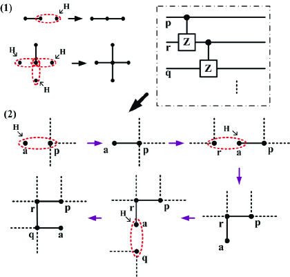
Figure 2: (color online) (1) Preparation of a linear and a star-shaped graph state. The red circle denotes an entangler operation, and H a Hadamard operation. The initial building blocks for the graph states are single photon qubits, as well as Bell pairs which can be prepared by the entangler in Fig.1 without using ancilla. (2) Realization of a 2-cascade CZ operation. The entangler first entangles photon $a$ and photon $p$ by putting $p$ at the position of $r$ in Fig. 1. Then, photon $a$ assists the connection of the entanglement bonds between photon $p$ and $r$, $r$ and $q$ in succession. It acts like a spider weaving these photons together into a string. A general cascade CZ operation like that in the dash-dotted line can be implemented in this fashion.

In the input state of Eq. (2), photon $a$ is specifically correlated to photon $p$ such that $|+\rangle_{a}$ ($|-\rangle_{a}$) is in the same terms with $|0\rangle_{p}$ ($|1\rangle_{p}$). After the operation described above, such correlation is transfered to between photon $a$ and $r$; see Eq. (7). One could use the output state as the input in the form of Eq. (2) to entangle the next photon to photon $r$, and so on. The operations of entangling a number of independent photons to a string can be therefore assisted by the same spider photon $a$, as the specific entanglement with the spider photon is transferred from photon to photon; see part (2) of Fig. 2 for a basic $2$-cascade entangler operation. The spider photon is the only ancilla for implementing a cascade entangler operation, and it will not be destroyed before we complete the whole operation.

Obviously, the starting piece or the Bell pair between the first photon $p_{1}$ and the spider photon $a$ (here we have no other photons in $|\psi_{1}\rangle,|\psi_{2}\rangle$ of Eq. (2)) can be prepared by the same entangler as well. Now photon $p_{1}$ should take the position of photon $r$ in Fig. 1. The coupling of the cross-Kerr nonlinearities in the same pattern, as well as the detection by the QND module, transforms the state $|+\rangle_{p_{1}}|+\rangle_{a}$ to either $|0\rangle_{p_{1}}|0\rangle_{a}+|1\rangle_{p_{1}}|1\rangle_{a}$ or $|0\rangle_{p_{1}}|1\rangle_{a}+|1\rangle_{p_{1}}|0\rangle_{a}$, which can be converted to $|0\rangle_{p_{1}}|+\rangle_{a}+|1\rangle_{p_{1}}|-\rangle_{a}$ by local operations. Compared with the strategy in Lin3 , all operations here can be performed by the same entangler in Fig. 1.

Moreover, extra entanglement links between qubits in an already connected piece can be built up by the entangler. One example of this case is that photon $p$ and $r$ are entangled to a third photon so that their total state is not separable. The entangler will operate in the same way except for processing a more general input like

$$|\Psi\rangle_{in} \left.=\left|\psi_{00}\right\rangle\left|0\right\rangle_{p}\left|0\right\rangle_{r}\left|+\right\rangle_{a}+\left|\psi_{01}\right\rangle\left|0\right\rangle_{p}\left|1\right\rangle_{r}\left|+\right\rangle_{a}\right.$$

$$\left.+\left|\psi_{10}\right\rangle\left|1\right\rangle_{p}\left|0\right\rangle_{r}\left|-\right\rangle_{a}+\left|\psi_{11}\right\rangle\left|1\right\rangle_{p}\left|1\right\rangle_{r}\left|-\right\rangle_{a}.\right.$$ (8)

This implies that spider photons can make circles by going through a same qubit in graph states for more than one time.

There is also a linear optical version for the cascade entangler; see Fig. 3. By the photon-photon interference via the polarization beam splitters and the coincident photon detection, the linear optical circuit effectively realizes a CZ operation as the nonlinear one in Fig. 1. Such linear optical cascade entangler only works with a success probability $1/2^{n}$ in generating a string of $n$ photonic qubits, but it could be used for experimental demonstration of this type of entangler.

Figure 3: (color online) Linear optical realization of the cascade CZ operation. Via the polarization beam splitters, the spider photon in the state $\left|+\right\rangle$ interferes with the photons p, r, q in succession. The PBS act as entanglers or parity gate, thus realizing a 2-cascade CZ operation associated with Hadamard operations performed on the ancilla between two PBS and the coincidence measurement.

III Generation of graph states

In the generation of graph states, we stipulate that the spider photons should move along the paths that do not retrace an already connected link; otherwise it will destroy the bonds by the operation of entangler. This requirement is the same as that for walking through the edges of a graph once and only once; c.f. the problem of Seven Bridges of Königsberg, a notable mathematics problem solved by L. Euler.

The generation strategy we have presented can be viewed as weaving up a graph network by spider photons following the above rule. One could have an optimal decomposition of a graph state, such that the number of parallel or separate operations for generating the state is minimized by letting one spider photon go through as many vertexes as possible. This spider photon could pass through a qubit in graph states for any number of times as long as it obeys the rule of not stepping on the already connected links, as a cascade entangler is able to process the most general input in Eq. (8). In what follows we will give a few examples of generating graph states by the weaving strategy.

The first example is a square-shaped 2D graph state. Without loss of generality, we demonstrate the preparation of a $5\times 5$ one in Fig. 4. The initial building blocks, the short chains of two or three qubits, can be prepared by the same cascade entangler beforehand or generated simultaneously with different entanglers, while the unlinked qubits will be connected to a single string from one of the initially linked. During the operation, the unlinked qubits are woven by a spider photon (not shown explicitly in the figure) in turn to the string, as it makes the indicated paths going through the qubits inside the square for more than one time. This string covers all entanglement links except for those initially connected.

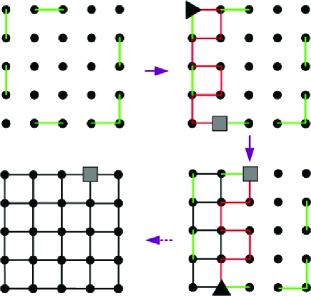
Figure 4: (color online) Generation of $5\times 5$ graph state. Some linear graph states (denoted by green lines) are prepared at the beginning as the building blocks. Then, one ancilla photon (not shown explicitly), which is entangled to one of the linear graph states, is used as the spider photon to connect the entanglement bonds. In each step, its starting point is marked by a triangle and its ending point marked by a square. The paths of the spider photon are denoted by red lines.

Figure 5: (color online) Generation of $4\times 4$ alveolate graph state. Some linear graph states are used as the building blocks. In each step, the starting point of the spider photon is marked by a triangle and its ending point marked by a square.

The generation of alveolate graph state dc-c1 ; alveolate , a special kind of 2D graph state, is similar. Following the rule for the spider photon, a general alveolate graph state can be generated as it walks through the paths denoted by red lines in Fig. 5.

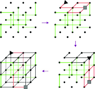
Figure 6: (color online) Generation of $3\times 3\times 3$ graph state. The building blacks used here are the star-shaped and linear graph states prepared as in Fig. (2.1), as well as the individual photonic qubits. In each step, the starting point of the spider photon is marked by a triangle and its ending point marked by a square.

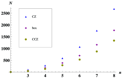
Figure 7: (color online) Comparison of the numbers of the individual entangler operations in generating an $n\times n\times n$ cubic graph state. The number by the cascade entangler (CCZ) in this paper is $N=3(n-1)n^{2}+1$. By the block by block (box) strategy in Lin3 , the corresponding number is $n=4(n-1)n^{2}-2n+1$, if $n$ is even; and $N=4(n-1)n^{2}-n+1$, if $n$ is odd. The corresponding number by the direct CZ operations on each entanglement bond is $N=6(n-1)n^{2}$.

The advantage of the weaving strategy is more obvious in 3D graph state generation. 3D graph states are proposed for the fault-tolerant one-way quantum computing 3D . The three dimension of a graph state means the cubically increasing entanglement bonds, which demand much more operations than in preparing 2D graph states. Here we use the example of $3\times 3\times 3$ graph state in Fig. 6 to illustrate the generation of 3D graph state by cascade CZ operations. The building blocks are two star-shaped graph states and one linear graph state prepared as in Fig. (2.1), as well as a Bell pair and the rest unconnected single-photon qubits. The star-shaped graph states and Bell pair are denoted with the green bonds in Fig. 6. All these pieces can be generated by the simultaneous operations of more entanglers, or by the same entangler beforehand or afterward. The passage of the spider photon is shown with the red lines in each step of Fig. 6. The spider photon keeps traveling side by side on the cubic until it connects all entanglement links other than the initially connected.

Only counting the number of the individual entangling operations in generating an $n\times n\times n$ graph state, this weaving strategy improves on other approaches by requiring less operations; see Fig. 7. Such improvement is due to the fact that the passage of a spider photon can be on different 2D planes of a cubic. Since the operations in generating each string $E_{i}$ can be bundled together by a cascade entangler, the actually number of separate operations in preparing an $n\times n\times n$ cubic graph state is in the order of that of the linked initial building blocks in Fig. 6, whose quantity is in the order of $n$. By our weaving strategy, therefore, the quantity of the necessary resource for preparing a 3D graph state only grows with the size number $n$ rather than its link number $n^{3}$.

IV Discussion and conclusion

The core element for our cascade entangler is a proper weak cross Kerr nonlinearity for entangling operations and in QND modules. The recent experimental progress on photonic XPM can be found in, e. g., chen ; fiber ; lo ; ex4 ; ex5 . More progress in the research of such photonic nonlinearity is expected in the near future.

Most of theoretical studies thus far (including the present one) adopt the simplified single mode treatment for XPM between photons and coherent states. This picture is criticized in shap2 , which considers the quantum noise effect due to the non-instantaneous response of nonlinear media. However, in the regime of very small conditional phase $\theta$, a multi-mode XPM from the instantaneous photonic interactions works almost in the same way as that of single mode approximation multi ; qft . Given a small conditional phase $\theta\ll 1$, our deterministic entangler should work in the regime of $\alpha\sin\theta\gg 1$. Such compatibility between a small conditional phase and a large average photon numbers of the qubus beams in the realistic multi-mode XPM is clarified in xpm , where we adopt a continuous-mode interacting quantum field model to show the validity of the single mode approximation in this regime.

We have illustrated how to apply cascade entangler operations to entangle independent single photons into arbitrary graph state. This approach is highly efficient and suitable to preparing the graph states of large number of qubits. It could make photon a suitable qubit for the realistic one-way quantum computing.

- (1) H. J. Briegel and R. Raussendorf, Phys. Rev. Lett. 86, 910 (2001).
- (2) R. Raussendorf and H. J. Briegel, Phys. Rev. Lett. 86, 5188 (2001).
- (3) R. Raussendorf, D. E. Browne and H. J. Briegel, Phys. Rev. A 68, 022312 (2003).
- (4) R. Raussendorf, J. Harrington and K. Goyal, Ann. Phys. 321, 2242 (2006).
- (5) M. A. Nielsen, Phys. Rev. Lett. 93, 040503 (2004).
- (6) D. E. Browne and T. Rudolph, Phys. Rev. Lett. 95, 010501 (2004).
- (7) G. Gilbert, M. Hamrick and Y. S. Weinstein, Phys. Rev. A 73, 064303 (2006).
- (8) T. P. Bodiya and L. M. Duan, Phys. Rev. Lett. 97, 143601 (2006).
- (9) J. Zhang and S. L. Braunstein, Phys. Rev. A 73, 032318 (2006).
- (10) N. C. Menicucci, P. van Loock, M. Gu, C. Weedbrook, T. C. Ralph and M. A. Nielsen, Phys. Rev. Lett. 97, 110501 (2006).
- (11) M. Gu, C. Weedbrook, N. C. Menicucci, T. C. Ralph and P. van Loock, Phys. Rev. A 79, 062318 (2009).
- (12) P. Walther, et al., Nature (London), 434, 169 (2005).
- (13) P. Walther, et al., Phys. Rev. Lett., 95, 020403 (2005).
- (14) N. Kiesel, et al., Phys. Rev. Lett., 95, 210502 (2005).
- (15) C. Y. Lu, et al., Nature Phys., 3, 91 (2007).
- (16) Y. Tokunaga, et al., Phys. Rev. Lett., 100, 210501 (2008).
- (17) W. B. Gao, et al., Phys. Rev. Lett., 104, 020501 (2010).
- (18) J. H. Shapiro, Phys. Rev. A 73, 062305 (2006).
- (19) J. Gea-Banacloche, Phys. Rev. A, 81, 043823 (2010).
- (20) B. He, A. MacRae, Y. Han, A. I. Lvovsky and C. Simon, Phys. Rev. A, 83, 022312 (2011).
- (21) B. He and A. Scherer, arXiv:1012.1683.
- (22) K. Nemoto and W. J. Munro, Phys. Rev. Lett. 93, 250502 (2004).
- (23) S. D. Barrett, P. Kok, K. Nemoto, R. G. Beausoleil, W. J. Munro and T. P. Spiller, Phys. Rev. A 71, 060302(R) (2005).
- (24) S. G. R. Louis, K. Nemoto, W. J. Munro and T. P. Spiller, Phys. Rev. A 75, 042323 (2007).
- (25) S. G. R. Louis, K. Nemoto, W. J. Munro and T. P. Spiller, New J. Phys. 9, 193 (2007).
- (26) C. Horsman, K. L. Brown, W. J. Munro, V. M. Kendon, Phys. Rev. A, 83, 042327 (2011).
- (27) W. J. Munro, K. Nemoto and T. P. Spiller, New J. Phys. 7, 137 (2005).
- (28) Q. Lin and B. He, Phys. Rev. A 82, 022331 (2010).
- (29) M. Hein, W. Dür, J. Eisert, R. Raussendorf, M. Van den Nest and H. J. Briegel, Proceedings of the International School of Physics “Enrico Fermi” on “Quantum Computers, Algorithms and Chaos” (2005); quant-ph/0602096.
- (30) B. He, Y.-H. Ren, and J. A. Bergou, Phys. Rev. A79, 052323 (2009).
- (31) B. He, Y.-H. Ren, and J. A. Bergou, J. Phys. B: At. Mol. Opt. Phys. 43, 025502 (2010).
- (32) Q. Lin, B. He, J. A. Bergou and Y. H. Ren, Phys. Rev. A 80, 042311 (2009).
- (33) Q. Lin and B. He, Phys. Rev. A 80, 042310 (2009).
- (34) Y. Y. Shi, L. M. Duan and G. Vidal, Phys. Rev. A 74, 022320 (2006).
- (35) Y. F. Chen, C. Y. Wang, S. H. Wang and I. A. Yu, Phys. Rev. Lett., 96, 043603 (2006).
- (36) N. Matsuda, et al., Nature Photonics, 3, 95 (2009).
- (37) H. Y. Lo, P. C. Su and Y. F. Chen, Phys. Rev. A, 81, 053829 (2010).
- (38) H. Y. Lo, et al., Phys. Rev. A, 83, 041804(R) (2011).
- (39) B. W. Shiau, M. C. Wu , C. C. Lin and Y. C. Chen, Phys. Rev. Lett., 106, 193006 (2011).
- (40) J. H. Shapiro and M. Razavi, New J. Phys. 9, 16 (2007).
- (41) B. He, Q. Lin and C. Simon, Phys. Rev. A, 83, 053826 (2011).