Quench dynamics of the topological quantum phase transition in the Wen-plaquette model

Abstract

We study the quench dynamics of the topological quantum phase transition in the two-dimensional transverse Wen-plaquette model, which has a phase transition from a $Z_{2}$ topologically ordered to a spin-polarized state. By mapping the Wen-plaquette model onto a one-dimensional quantum Ising model, we calculate the expectation value of the plaquette operator $F_{i}$ during a slowly quenching process from a topologically ordered state. A logarithmic scaling law of quench dynamics near the quantum phase transition is found, which is analogous to the well-known static critical behavior of the specific heat in the one-dimensional quantum Ising model.

I Introduction

Ultracold atoms provide an ideal platform for experimental studies of the time evolution of quantum systems, and make it desirable for related theoretical explorations on dynamics of quantum phase transitions in various models. These explorations mainly focus on nonequilibrium dynamics in quantum systems which undergo a quantum phase transition when a system parameter is varied (quantum quench)Pol_colloquium . These experimental and theoretical studies can potentially help to pave the way for future technologies and provide a deeper understanding of quantum many-body physics, particularly the universal scaling behavior in the quench dynamics.

Recently, a new type of phase transition, the so-called topological quantum phase transition (TQPT) has attracted considerable research attentionWenbook ; wen3 ; wen4 ; wen1 ; Kitaev ; nayak ; lidar ; chamon ; xiang ; yujing ; vid1 ; vid2 . TQPT is a kind of phase transition between two quantum states with the same symmetry. It is fundamentally different from the usual symmetry-breaking phase transition, and involves a new type of order — topological order, as introduced by WenWenTo1 . In such an ordered state, there is no local order parameter, and the state is robust against arbitrary local perturbations. On this basis, quantum systems with topological order have been proposed to build robust quantum memoriesKitaev and topological quantum computer (TQC)kou1 ; kou2 . In Refs.kou1 ; kou2 , it was shown that the pure state of topological order can be obtained via an adiabatical and continuous evolution process from a non-topologically ordered state and further be used as the initial state for TQC. Nevertheless, the detailed dynamics of such a quench process, particularly the universal scaling behavior near TQPT, has not been studied yet.

In the last decade, several exactly solvable spin models with topological order were found, such as the toric-code modelKitaev , the Wen-plaquette modelWen and the Kitaev model on a hexagonal latticeKitaev2 . These spin models provide a framework to study the TQPT and its quench dynamics. Thus, in recent years, some research groups have studied the quench dynamics of TQPT in the Kitaev model (e.g. Mondal et al. quh-Kiv ) or the toric-code model (e.g. Tsomokos  et al. quh-tc ). Mondal et al. found a relationship between the quench rate and the defect density in the one-dimensional (1D) and two-dimensional (2D) Kitaev model in the limit of slow quench rate and generalized the result to the defect density of a $d$ dimensional quantum model. Tsomokos et al. investigated how a topologically ordered ground state in the toric-code model reacts to rapid quenches. They tested several cases and showed which kind of quench can preserve or suppress the topological order.

In this work, we study the quench dynamics of TQPT from a topologically ordered state to a non-topological order in the Wen-plaquette model. To characterize the phase transition, we calculate the expectation value of plaquette operator $F_{i}$ during the quenching process, which is related to the number of quasiparticles in the topologically ordered state. Our results provide helpful information about the whole quenching process.

The remaining of this paper is organized as follows. Section II describes an exact mapping from the 2D transverse Wen-plaquette model onto the 1D Ising chain. In Sec. III, we study the TQPT of the 2D transverse Wen-plaquette model and give some results about its order parameters. In Sec. IV, we give the solutions to the dynamics of TQPT in the transverse Wen-plaquette model. A brief discussion is given in Sec. V.

II Mapping the transverse Wen-plaquette onto Ising model

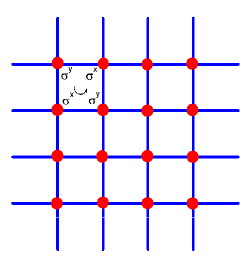
Figure 1: (Color online) The lattice where Wen-plaquette model is located. A plaquette is defined by $F_{i}=\tau_{i}^{y}\tau_{i+\hat{x}}^{x}\tau_{i+\hat{x}+\hat{y}}^{y}\tau_{i+\hat{y}}^{x}$.

We start with the Hamiltonian of the Wen-plaquette model on a square lattice with periodic boundary conditions in both directions:

$$H_{W}=-g\sum_{i}F_{i},\quad F_{i}=\tau_{i}^{y}\tau_{i+\hat{x}}^{x}\tau_{i+\hat{x}+\hat{y}}^{y}\tau_{i+\hat{y}}^{x},$$ (1)

where $\tau_{i}^{x}$ and $\tau_{i}^{y}$ are Pauli operators on site $i$, $\hat{x}$ and $\hat{y}$ are the unit vectors in x-axis and y-axis, respectively (see Fig. 1). Because of the commutativity of $H$ and $F_{i}$, the energy eigenstates can be labeled by the eigenstates of $F_{i}$. We can easily find $F_{i}^{2}=1$, so the eigenvalues of $F_{i}$ are $F_{i}=1$ and $F_{i}=-1$, which gives the exact ground state energy. In the case of $g>0$, the ground state is $F_{i}=1$ for every plaquette, and the elementary excitation is $F_{i}=-1$ on one plaquette (denoted by $i$) with an energy gap $E_{g}-E_{0}=2g$. On an even-by-even lattice, there are two types of plaquettes — the even plaquettes and the odd plaquettes respectively. As a result, one may define two kinds of bosonic quasiparticles: $Z_{2}$ charge and $Z_{2}$ vortex (see detailed calculations in Ref. Wen or Ref. Wenbook ). A $Z_{2}$ charge is defined by $F_{i}=-1$ on an even sub-plaquette while a $Z_{2}$ vortex defined by $F_{i}=-1$ on an odd. Thus a fermion can be regarded as the bound state of a $Z_{2}$ charge and a $Z_{2}$ vortex.

Now we consider the Wen-plaquette model in a transverse field, which is defined by:

$$H_{W}^{\prime}=-g\sum_{i}F_{i}-J\sum_{i}\tau_{i}^{x}.$$ (2)

This model on a square lattice can be mapped onto the 1D quantum Ising model with the Hamiltonian yujing

$$H_{I}=-\sum_{n=1}^{N}(g_{I}{\sigma}_{n}^{x}+{\sigma}_{n}^{z}{\sigma}_{n}^{z}),$$ (3)

where $\sigma_{n}^{x}$ and $\sigma_{n}^{z}$ are Pauli operators.

To derive the mapping, one can calculate the commutation relations (see detailed calculations in Appendix):

$$[F_{i},\tau_{j}^{x}]=2F_{i}\tau_{j}^{x}(\delta_{i,j-\hat{x}}+\delta_{i,j-\hat{y}}),$$

$$[F_{i},F_{j}]=0,$$

$$[\tau_{i}^{x},\tau_{j}^{x}]=0.$$ (4)

These relations correspond to those in Ising model:

$$[\sigma_{i}^{x},\sigma_{j}^{z}\sigma_{j+1}^{z}]=2\sigma_{i}^{x}\sigma_{j}^{z}\sigma_{j+1}^{z}(\delta_{i,j}+\delta_{i,j+1}),$$

$$[\sigma_{i}^{x},\sigma_{j}^{x}]=0,$$

$$[\sigma_{i}^{z}\sigma_{i+1}^{z},\sigma_{j}^{z}\sigma_{j+1}^{z}]=0.$$ (5)

Then we obtain the mapping

$$F_{i}\leftrightarrow\sigma_{i}^{x},\quad\tau_{i}^{x}\leftrightarrow\sigma_{i}^{z}\sigma_{i+1}^{z}.$$ (6)

Accordingly, the Hamiltonian (2) can be mapped onto the 1D quantum Ising model like following:

$$H_{W}^{\prime}\rightarrow-\sum_{\alpha}\sum_{i}(g\sigma_{\alpha i}^{x}+J\sigma_{\alpha i}^{z}\sigma_{\alpha i+1}^{z}),$$ (7)

where the subscript $\alpha$ implies there is one or more Ising chains. The number of Ising chains is determined by the size of the square lattice for the Wen-plaquette model (see Ref.yujing ). Since the Ising chains decouple from each other, we can consider only one Ising chain without loss of generality, and reduce the Hamiltonian (7) to

$$H_{W}^{\prime}=-J\sum_{i}(g_{W}\sigma_{i}^{x}+\sigma_{i}^{z}\sigma_{i+1}^{z}),\quad g_{W}=\frac{g}{J}.$$ (8)

Then we may explore the quantum properties of the original Wen-plaquette model by studying the corresponding 1D Ising model.

III String order parameters in Wen-plaquette model

For the 1D transverse Ising model (3), there are two phases: in the limit of $g_{I}\gg 1$, the ground state is a paramagnet with all spins polarized along x-axis, $\left\langle\sigma_{i}^{x}\right\rangle\rightarrow 1$; in the limit of $g_{I}\ll 1$, there are two degenerate ferromagnetic ground states with all spins along positive or negative z-axis and $\left\langle\sigma_{i}^{x}\right\rangle\rightarrow 0$. Consequently, in Hamiltonian (8), there is a quantum critical point atBaxter

$$g_{W}=\frac{g}{J}=1$$ (9)

that divides the two phases. Accordingly, the original transverse Wen-plaquette model also has two phases separated by this quantum critical point — in the region of $g_{W}>1$, the system is a topologically ordered state; in the region of $g_{W}<1,$ it’s a spin-polarized state.

Noting that the local order parameters cannot be used to learn the nature of TQPT any more, we introduce two non-local order parameters $\psi_{1}$ and $\psi_{2}$ as string order parameters (SOP’s) in the transverse Wen-plaquette model. They are defined by the expectations of string operators $\prod_{i}F_{i}$ and $\prod_{i}\tau_{i}^{x}$ with $i$ as the site index along a string in the diagonal directionyujing , i.e. $\psi_{1}\equiv\left\langle\prod_{i}F_{i}\right\rangle$ and $\psi_{2}\equiv\left\langle\prod_{i}\tau_{i}^{x}\right\rangle$, respectively.

We then calculate these two SOP’s by using the mapping in Eq.(6). For $\psi_{2}$, one has

$$\psi_{2}=\left\langle\prod_{i}\tau_{i}^{x}\right\rangle=\left\langle\sigma_{1}^{z}\sigma_{2}^{z}\sigma_{2}^{z}\sigma_{3}^{z}\cdots\sigma_{n-1}^{z}\sigma_{n}^{z}\right\rangle=\left\langle\sigma_{1}^{z}\sigma_{n}^{z}\right\rangle,$$ (10)

which becomes the correlation of two spins in the Ising chain of length $n$. By employing the Jordan-Wigner transformation

$$\sigma_{n}^{x}=1-2c_{n}^{\dagger}c_{n},\quad\sigma_{n}^{z}=-(c_{n}+c_{n}^{\dagger})\nu,$$ (11)

where

$$\nu\equiv\prod_{m<n}(1-2c_{m}^{\dagger}c_{m})=\prod_{m<n}(c_{m}c_{m}^{\dagger}-c_{m}^{\dagger}c_{m})=\prod_{m<n}A_{m}B_{m},$$ (12)

where $A_{m}=c_{m}^{\dagger}+c_{m}$, $B_{m}=c_{m}^{\dagger}-c_{m}$, $c^{\dagger}_{m}$ and $c_{m}$ are the creation and annihilation operators for fermions, we obtain

$$\psi_{2} =\left\langle\sigma_{1}^{z}\sigma_{n}^{z}\right\rangle=\left\langle(c_{1}+c_{1}^{\dagger})\nu(c_{n}+c_{n}^{\dagger})\right\rangle$$

$$=\left\langle B_{1}A_{2}B_{2}\cdots B_{n-1}A_{n}\right\rangle.$$ (13)

Following the Wick’s theorem, we can transform Eq.(III) into a Toeplitz determinant asbook20

$$\left|\begin{array}[c]{cccc}G_{12}&G_{13}&\cdots&G_{1n}\\ G_{22}&G_{23}&\cdots&G_{2n}\\ \vdots&\vdots&\ddots&\vdots\\ G_{n-1,2}&G_{n-1,3}&\cdots&G_{n-1,n}\end{array}\right|,$$ (14)

where

$$G_{ij}=-\frac{1}{2\pi}\int_{-\pi}^{\pi}\mathrm{d}k\frac{g_{W}-\cos k-i\sin k}{\sqrt{(g_{W}-\cos k)^{2}+\sin^{2}k}}e^{ik(i-j)}.$$ (15)

In the thermodynamic limit $N\rightarrow\infty$, we have (see Ref. McCoy1 or Ref. McCoy2 )

$$\psi_{2}\sim\left\{\begin{array}[c]{ll}(1-g_{W}^{2})^{1/4}&\text{when $g_{W}<1$}\\ 0&\text{when $g_{W}\geq 1$}\end{array}\right..$$ (16)

The exponent $1/4$ here agrees with the critical exponent $2\beta/\nu=1/4$ (see Ref.Baxter ).

By the same method we can obtain the result of $\psi_{1}$,

$$\psi_{1}=\left\langle\prod_{i}F_{i}\right\rangle=\left\langle\prod_{i}\sigma_{i}^{x}\right\rangle.$$ (17)

In addition, we can take advantage of the duality of 1D Ising model (see Ref. book20 ) :

$$s_{i}^{x}=\sigma_{i}^{z}\sigma_{i+1}^{z}\quad\text{and}\quad s_{i}^{z}=\prod_{k<i}\sigma_{k}^{x}.$$ (18)

Thus the result in Eq.(17) is turned into $\psi_{1}=m$, where $m\equiv\left\langle\sigma_{i}^{z}\right\rangle$ is the spontaneous magnetization. We can find that when $N\rightarrow\infty$, the spin correlation (10) is the square of $m$. Consequently, from Eq.(16), we have

$$\psi_{1}\sim\left\{\begin{array}[c]{ll}0&\text{when $g_{W}\leq 1$}\\ (1-g_{W}^{-2})^{1/8}&\text{when $g_{W}>1$}\end{array}\right..$$ (19)

From the calculations above, one may notice that the non-local SOPs in a 2D transverse Wen-plaquette model are transformed to the local order parameters in the dual 1D Ising model.

IV Quench dynamics of TQPT

In this section we study the dynamics of TQPT in the transverse Wen-plaquette model. The Kibble-Zurek mechanism (KZM)Kibble ; Zurek is a general theory to explore the dynamics of second order phase transitions including the quantum case. According to KZM, during a quench-induced phase transition, the system undergoes three stages of evolution: adiabatic–pulse–adiabatic. It predicts that the density of topological defects, which are generated by the pulse evolution, is a function of quench time.

We can solve the dynamic problems in the Wen-plaquette model by taking a sequence of transformations as in Ref. quench . First, through the Jordan-Wigner transformation (11), the spin operators $\sigma_{i}^{x,z}$ are represented by fermionic operators $c_{n}$. Second, the operators $c_{n}$ are Fourier transformed into the momentum space:

$$c_{n}=\frac{e^{-i\pi/4}}{\sqrt{N}}\sum_{k}c_{k}e^{ikn}.$$ (20)

Third, after Bogoliubov transformation, one have

$$c_{k}=u_{k}\eta_{k}+v_{-k}^{\ast}\eta_{-k}^{\dagger},$$ (21)

where $\eta_{k}$ and $\eta_{k}^{\dagger}$ are fermionic operators. For dynamic problems, the expression (21) becomes

$$c_{k}(t)=u_{k}(t)\widetilde{\eta}_{k}+v_{-k}^{\ast}(t)\widetilde{\eta}_{-k}^{\dagger}.$$ (22)

Now, a dynamic solution can be written in the form of Bogoliubov mode $(u_{k}(t),$ $v_{k}(t))$ after this whole transformation procedure.

By this method, the dynamics of the quantum Ising model can be expressed as the time evolution of the Bogoliubov mode via so-called Bogoliubov-de Gennes dynamic equations (see Ref. quench ):

$$\left\{\begin{array}[c]{l}i\hbar\mathrm{d}u_{k}/\mathrm{d}t=+2(g_{I}(t)-\cos k)u_{k}+2\sin kv_{k}\\ i\hbar\mathrm{d}v_{k}/\mathrm{d}t=-2(g_{I}(t)-\cos k)v_{k}+2\sin ku_{k}\end{array}\right..$$ (23)

Consider a linear quench, i.e.

$$g_{I}(t<0)=-\frac{t}{{\tau}_{Q}},$$ (24)

where $t$ varies from $-\infty$ to $0$ and the quench time $\tau_{Q}$ characterizes the quench rate (defined by $1/\tau_{Q}$). Equations (23) can be transformed into the form of Landau-Zener (LZ) modelLZmodel (the connection between the KZM and the LZ model can be found in Ref. Dam ; Dam-Zuk ) :

$$\left\{\begin{array}[c]{l}i\hbar\mathrm{d}u_{k}/\mathrm{d}\tau=-\frac{1}{2}(\tau\Delta_{k})u_{k}+\frac{1}{2}v_{k}\\ i\hbar\mathrm{d}v_{k}/\mathrm{d}\tau=+\frac{1}{2}(\tau\Delta_{k})v_{k}+\frac{1}{2}u_{k}\end{array}\right.,$$ (25)

where

$$\tau=4\tau_{Q}\sin k(\frac{t}{\tau_{Q}}+\cos k),$$

and

$$\Delta_{k}^{-1}=4\tau_{Q}\sin^{2}k.$$

From equations (25), we derive a second order differential equation for $v_{k}$:

$$\frac{\mathrm{d}^{2}v_{k}}{\mathrm{d}\tau^{2}}+(\frac{1}{4}\tau^{2}\Delta^{2}_{k}+\frac{i\Delta_{k}}{2}+\frac{1}{4})v_{k}=0.$$ (26)

After the substitutions

$$s=\frac{1}{4i\Delta_{k}}\quad\text{and}\quad z=\sqrt{\Delta_{k}}\tau e^{i\pi/4},$$ (27)

we have

$$\frac{\mathrm{d}^{2}v_{k}(z)}{\mathrm{d}z^{2}}+(s+\frac{1}{2}-\frac{1}{4}z^{2})v_{k}(z)=0.$$ (28)

This kind of differential equation has a general solution

$$\begin{array}[c]{l}v_{k}(\tau)=-[aD_{-s-1}(-iz)+bD_{-s-1}(iz)],\\ u_{k}(\tau)=(-\Delta_{k}\tau+2i\frac{\partial}{\partial\tau})v_{k}(\tau),\end{array}$$ (29)

where $D_{m}(x)$ is the so-called parabolic cylinder function (PCF) or Weber-Hermite functionWhi-Wat .

According to the boundary conditions and the characters of the PCF, one may derive the approximative solutions to equations (28) at the end of linear quench for $t=0$ (See Ref. quench ):

$$\begin{array}[c]{l}{|u_{k}|}^{2}=\frac{1-\cos k}{2}+e^{-2\pi\tau_{Q}\sin^{2}k},\\ {|v_{k}|}^{2}=1-{|u_{k}|}^{2},\\ u_{k}v_{k}^{\ast}=\frac{1}{2}\sin k+sgn(k)e^{-\pi\tau_{Q}\sin^{2}k}\sqrt{1-e^{-\pi\tau_{Q}\sin^{2}k}}e^{i\varphi_{k}},\end{array}$$ (30)

with the condition $\tau_{Q}\gg 1$.

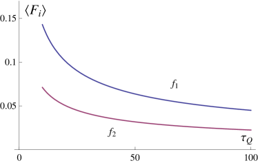
Figure 2: (Color online) The expectation value of $F_{i}$ at $t=0$ varying with the quench time $\tau_{Q}$, where $f_{1}=1-\frac{1}{\pi}\int_{-\pi}^{\pi}\mathrm{d}k(\frac{1+\cos k}{2}-e^{-2\pi\tau_{Q}\sin^{2}k})$ and the approximative result $f_{2}=\frac{1}{\pi\sqrt{2\tau_{Q}}}$.

Now we calculate the dynamic solutions in the Wen-plaquette model via the same transformation procedure plus the mapping (6). We shall also consider

$$g_{W}(t<0)=-\frac{t}{{\tau}_{Q}}.$$ (31)

The quenching process can be set as tuning the strength of the transverse field from zero to very large compared with the coupling constant $g$. The phase transition is thus from a topologically ordered state to a spin-polarized state during the time-evolution from $t\rightarrow-\infty$ to $t=0$.

First, we calculate the expectation value of $F_{i}$ after the quenching process. From the Jordan-Wigner transformation, $\sigma_{n}^{x}=1-2c_{n}^{\dagger}c_{n}$, we have

$$\left\langle F_{i}\right\rangle\rightarrow\left\langle\sigma_{n}^{x}\right\rangle=\left\langle\left(1-2c_{n}^{\dagger}c_{n}\right)\right\rangle.$$

Through the Fourier transformation, we express $c_{m}^{\dagger}c_{n}$ in momentum space

$$c_{m}^{\dagger}c_{n}=\frac{1}{2\pi}\int_{-\pi}^{\pi}\mathrm{d}k\int_{-\pi}^{\pi}\mathrm{d}k^{\prime}c_{k}^{\dagger}c_{k^{\prime}}e^{i(k^{\prime}n-km)}.$$ (32)

After the Bogoliubov transformation (21), we obtainintro1

$$\langle c_{m}^{\dagger}c_{n}\rangle =\frac{1}{2\pi}\int_{-\pi}^{\pi}\mathrm{d}k\int_{-\pi}^{\pi}\mathrm{d}k^{\prime}e^{i(k^{\prime}n-km)}v_{-k}v_{-k}^{\ast}\delta_{k,k^{\prime}}$$

$$=\frac{1}{2\pi}\int_{-\pi}^{\pi}\mathrm{d}k|v_{k}|^{2}e^{ik(n-m)}.$$ (33)

From the solutions (30), we derive

$$\left\langle F_{i}\right\rangle \rightarrow\left\langle\sigma_{n}^{x}\right\rangle=1-2\cdot\frac{1}{2\pi}\int_{-\pi}^{\pi}\mathrm{d}k(\frac{1+\cos k}{2}$$

$$-e^{-2\pi\tau_{Q}\sin^{2}k})\overset{\tau_{Q}\gg 1}{\simeq}\frac{1}{\pi\sqrt{2\tau_{Q}}}.$$ (34)

We can see the original state in the limit of $g\gg 1$, which is a topological ground state with $\left\langle F_{i}\right\rangle\rightarrow\left\langle\sigma_{n}^{x}\right\rangle\rightarrow 1$, will finally evolve into the trivial spin-polarized state with $\left\langle F_{i}\right\rangle\rightarrow\left\langle\sigma_{n}^{x}\right\rangle\rightarrow 0$. Figure 2 shows how the expectation value of $F_{i}$ at the end of quenching process ($t=0$) varies with the quench rate.

We can obtain the the numbers of $Z_{2}$ charges and $Z_{2}$ vortices by defining

$$\mathcal{N}_{c}\equiv\frac{1}{2}\sum_{i\in\mathrm{even}}(1-F_{i})=\sum_{i\in\mathrm{even}}c_{i}^{\dagger}c_{i}$$ (35)

and

$$\quad\mathcal{N}_{v}\equiv\frac{1}{2}\sum_{i\in\mathrm{odd}}(1-F_{i})=\sum_{i\in\mathrm{odd}}c_{i}^{\dagger}c_{i},$$

respectively. Before the quench, the system is in a topological ground state. There is no quasiparticles ($N_{c}\equiv\langle\mathcal{N}_{c}\rangle=0$, $N_{v}\equiv\langle\mathcal{N}_{v}\rangle=0$), so we have $F_{i}=1$ for all plaquettes. At the end of the quench, we can also calculate the density of plaquettes $F_{i}=-1$intro2 by

$$n= \frac{1}{2N}\langle\sum_{i}(1-F_{i})\rangle=\frac{1}{2\pi}\int_{-\pi}^{\pi}\mathrm{d}k(\frac{1+\cos k}{2}$$

$$-e^{-2\pi\tau_{Q}\sin^{2}k})\overset{\tau_{Q}\gg 1}{\simeq}\frac{1}{2}-\frac{1}{2\pi\sqrt{2\tau_{Q}}}.$$ (36)

It is obvious that when $\tau_{Q}\rightarrow\infty$, half of the plaquettes will be turned into $F_{i}=-1$, which implies $\left\langle F_{i}\right\rangle\rightarrow 0.$

However, this result cannot give us any information about the quenching process or the critical behaviors. In order to obtain such information, we find that, for $\tau_{Q}\gg 1$, the expression

$$|v_{k}(t)|^{2}=\frac{1}{2}(1+\frac{\cos k+t/\tau_{Q}}{\sqrt{1+2t/\tau\cos k+(t/\tau_{Q})^{2}}})-e^{-2\pi\tau_{Q}\sin^{2}k}$$ (37)

is a time-dependent approximate function for the general solution $|v_{k}(\tau)|^{2}$ in Eq.(29), if we cut off the negative part of the curve (see Fig. 3).

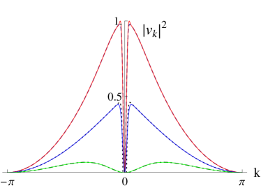
Figure 3: (Color online) The colored curves represent $|v_{k}(\tau)|^{2}$ in the original form of the PCF varying with momenta k from $-\pi$ to $\pi$, where the red one is at $t=-0.5\tau_{Q}$, the blue at $t=-\tau_{Q}$, the green at $t=-2\tau_{Q}$ with $\tau_{Q}=50$ in all the three cases. The dashed, dotted and dot-dashed curves, respectively, represent the approximate function for $|v_{k}(\tau)|^{2}$ with corresponding parameters, with the negative parts under the x-axis being cut off. They match with the colored curves very well

By using this approximate function, we calculate the value $\left\langle F_{i}\right\rangle$ during the quenching process as a function of the time $t$ near the quantum critical point. The result is shown in Fig. 4.

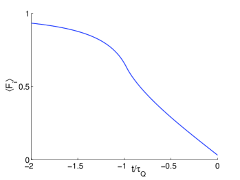
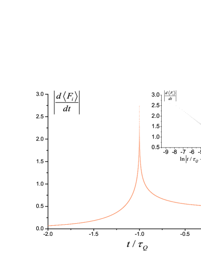
Figure 4: (Color online) The expectation value of $F_{i}$ during the quenching process varying from $t=-2\tau_{Q}$ to $t=0$ with $\tau_{Q}=50$ and the absolute value of the slope ($|\frac{\mathrm{d}\langle F_{i}\rangle}{\mathrm{d}t}|$) corresponding to the curve above. The small graph shows $|\frac{\mathrm{d}\langle F_{i}\rangle}{\mathrm{d}t}|\sim\ln|t/\tau_{Q}+1|$ from both sides approaching the critical point $t=-\tau_{Q}$.

Further calculations show that the derivative of the expectation-value $\left\langle F_{i}\right\rangle$ diverges at point $t=t_{c}=-\tau_{Q}$ as $\frac{\mathrm{d}\langle F_{i}\rangle}{\mathrm{d}t}\rightarrow-\infty$, which characterizes the critical point. In particular, we obtain a logarithmic scaling law of quench dynamics near the quantum phase transition as

$$\frac{\mathrm{d}\langle F_{i}\rangle}{\mathrm{d}t}\sim\ln|t-t_{c}|.$$ (38)

Such a dynamics is analogous to the static scaling behavior of the specific heat near the critical point for the 1D quantum Ising model.

The physical picture can be described as follows. At beginning, the external field is weak and can be treated as a perturbation, which creates vortices or charges and drives them to move around and annihilate each other. As a result, the density of quasiparticles remains small. As the strength of the field continuous to grow, the density of plaquettes $F_{i}=-1$ increases rapidly near the point $g_{W}=1$ (that is $t=-\tau_{Q}$). The rate of density-changing diverges with a logarithmic scaling law. Finally, at the end of the quench, the field becomes so strong that the vortices and charges are all confined and cannot be treated as quasiparticles. If the quenching process is infinitely slow, half of the plaquttes overturns.

In addition we shall notice that only the linear quench is considered here. However, for other cases, our method is not reliable. Inspired by other papers on quantum quench in the toric-code model (e.g. Rahmani et al. Rah-Cha , where a sudden quench is studied), we can study the quench problems more generally through the time evolution of the entanglement entropy in the Wen-plaquette model. Nevertheless, we will not consider this in this work.

V Conclusion

In summary, we study the dynamics of TQPT caused by a linear quench in the transverse Wen-plaquette model. We first show how to derive the mapping from the 2D Wen-plaquette onto the 1D Ising model by comparing their commutation relations. Based on this mapping, we point out the quantum critical point in the transverse Wen-plaquette model and calculate its non-local order parameters. We then calculate the expectation value of $F_{i}$ at the end of the quench, and further show how this value varies during the whole process. In particular, we find a logarithmic scaling law of quenching process near the TQPT.

Finally we address the realization of the Wen-plaquette model in an optical lattice of cold atoms. Because the Wen-plaquette model can be regarded as an effective model of the Kitaev model on a two dimensional hexagonal lattice, one may first realize the Kitaev model. The Hamiltonian of the Kitaev model isKitaev2

$$\mathrm{H}=\sum_{j+l=\text{even}}(\mathrm{J}_{x}\sigma_{j,l}^{x}\sigma_{j+1,l}^{x}+\mathrm{J}_{y}\sigma_{j-1,l}^{y}\sigma_{j,l}^{y}+\mathrm{J}_{z}\sigma_{j,l}^{z}\sigma_{j,l+1}^{z})$$ (39)

where $j$ and $l$ denote the column and row indices of the lattice. In the limit of $\mathrm{J}_{x}\mathrm{\gg J}_{z}\sim\mathrm{J}_{y}$ in this model, the effective Hamiltonian of Kitaev model is simplified into that of the Wen-plaquette model as

$$H_{0}=-\frac{\mathrm{J}_{z}^{2}\mathrm{J}_{y}^{2}}{16|\mathrm{J}_{x}|^{3}}\sum_{i}\sigma_{\text{left}(i)}^{x}\sigma_{\text{right}(i)}^{x}\sigma_{\text{up}(i)}^{y}\sigma_{\text{down}(i)}^{y}.$$ (40)

Then one can use the Kitaev model in the limit $\mathrm{J}_{x}\mathrm{\gg J}_{z}\sim\mathrm{J}_{y}$ on a torus to do the TQC. The realization of the Kitaev model on the 2D hexagonal lattice has been proposed in Ref.du ; zo1 . The essential idea realizing the Kitaev model is to induce and control virtual spin-dependent tunneling between neighboring atoms in the lattice that results in a controllable Heisenberg exchange interaction.

The authors acknowledge that this research is supported by NFSC Grant No. 10874017, 10975127, National Basic Research Program of China (973 Program) under the grant No. 2011CB92180, the Anhui Provincial Natural Science Foundation under Grant No. 090416224, and the Chinese Academy of Sciences.

Appendix

In this part, we give detailed calculations about commutation relations (II), which is related to the consistency between Wen-plaquette model and Ising model.

The key point is to calculate $[F_{i},F_{j}]$,

$$[F_{i},F_{j}]$$

$$=[\tau_{i}^{x}\tau_{i+\hat{x}}^{y}\tau_{i+\hat{y}+\hat{x}}^{x}\tau_{i+\hat{y}}^{y},\tau_{j}^{x}\tau_{j+\hat{x}}^{y}\tau_{j+\hat{y}+\hat{x}}^{x}\tau_{j+\hat{y}}^{y}]$$

$$=[\tau_{i}^{x},\tau_{j}^{x}\tau_{j+\hat{x}}^{y}\tau_{j+\hat{y}+\hat{x}}^{x}\tau_{j+\hat{y}}^{y}]\tau_{i+\hat{x}}^{y}\tau_{i+\hat{y}+\hat{x}}^{x}\tau_{i+\hat{y}}^{y}+\tau_{i}^{x}$$

$$[\tau_{i+\hat{x}}^{y},\tau_{j}^{x}\tau_{j+\hat{x}}^{y}\tau_{j+\hat{y}+\hat{x}}^{x}\tau_{j+\hat{y}}^{y}]\tau_{i+\hat{y}+\hat{x}}^{x}\tau_{i+\hat{y}}^{y}+\tau_{i}^{x}\tau_{i+\hat{x}}^{y}$$

$$[\tau_{i+\hat{y}+\hat{x}}^{x},\tau_{j}^{x}\tau_{j+\hat{x}}^{y}\tau_{j+\hat{y}+\hat{x}}^{x}\tau_{j+\hat{y}}^{y}]\tau_{i+\hat{y}}^{y}+\tau_{i}^{x}\tau_{i+\hat{x}}^{y}\tau_{i+\hat{y}+\hat{x}}^{x}$$

$$[\tau_{i+\hat{y}}^{y},\tau_{j}^{x}\tau_{j+\hat{x}}^{y}\tau_{j+\hat{y}+\hat{x}}^{x}\tau_{j+\hat{y}}^{y}].$$ (41)

According to the commutation relations of Pauli operators,

$$[\tau_{i}^{x},\tau_{j}^{x}\tau_{j+\hat{x}}^{y}\tau_{j+\hat{y}+\hat{x}}^{x}\tau_{j+\hat{y}}^{y}]$$

$$=[\tau_{i}^{x},\tau_{j}^{x}]\tau_{j+\hat{x}}^{y}\tau_{j+\hat{y}+\hat{x}}^{x}\tau_{j+\hat{y}}^{y}+\tau_{j}^{x}[\tau_{i}^{x},\tau_{j+\hat{x}}^{y}]\tau_{j+\hat{y}+\hat{x}}^{x}\tau_{j+\hat{y}}^{y}$$

$$+\tau_{j}^{x}\tau_{j+\hat{x}}^{y}[\tau_{i}^{x},\tau_{j+\hat{y}+\hat{x}}^{x}]\tau_{j+\hat{y}}^{y}+\tau_{j}^{x}\tau_{j+\hat{x}}^{y}\tau_{j+\hat{y}+\hat{x}}^{x}[\tau_{i}^{x},\tau_{j+\hat{y}}^{y}]$$

$$=2i\delta_{i,j+\hat{x}}\tau_{j}^{x}\tau_{i}^{z}\tau_{j+\hat{y}+\hat{x}}^{x}\tau_{j+\hat{y}}^{y}+2i\delta_{i,j+\hat{y}}\tau_{j}^{x}\tau_{j+\hat{x}}^{y}\tau_{j+\hat{y}+\hat{x}}^{x}\tau_{i}^{z};$$

$$[\tau_{i+\hat{x}}^{y},\tau_{j}^{x}\tau_{j+\hat{x}}^{y}\tau_{j+\hat{y}+\hat{x}}^{x}\tau_{j+\hat{y}}^{y}]$$

$$=[\tau_{i+\hat{x}}^{y},\tau_{j}^{x}]\tau_{j+\hat{x}}^{y}\tau_{j+\hat{y}+\hat{x}}^{x}\tau_{j+\hat{y}}^{y}+\tau_{j}^{x}[\tau_{i+\hat{x}}^{y},\tau_{j+\hat{x}}^{y}]\tau_{j+\hat{y}+\hat{x}}^{x}\tau_{j+\hat{y}}^{y}$$

$$+\tau_{j}^{x}\tau_{j+\hat{x}}^{y}[\tau_{i+\hat{x}}^{y},\tau_{j+\hat{y}+\hat{x}}^{x}]\tau_{j+\hat{y}}^{y}+\tau_{j}^{x}\tau_{j+\hat{x}}^{y}\tau_{j+\hat{y}+\hat{x}}^{x}[\tau_{i+\hat{x}}^{y},\tau_{j+\hat{y}}^{y}]$$

$$=-2i\delta_{i+\hat{x},j}\tau_{j}^{z}\tau_{j+\hat{x}}^{y}\tau_{j+\hat{y}+\hat{x}}^{x}\tau_{j+\hat{y}}^{y}-2i\delta_{i,j+\hat{y}}\tau_{j}^{x}\tau_{j+\hat{x}}^{y}\tau_{j+\hat{y}+\hat{x}}^{z}$$

$$\tau_{j+\hat{y}}^{y};$$ (43)

$$[\tau_{i+\hat{x}+\hat{x}}^{x},\tau_{j}^{x}\tau_{j+\hat{x}}^{y}\tau_{j+\hat{y}+\hat{x}}^{x}\tau_{j+\hat{y}}^{y}]$$

$$=[\tau_{i+\hat{x}+\hat{x}}^{x},\tau_{j}^{x}]\tau_{j+\hat{x}}^{y}\tau_{j+\hat{y}+\hat{x}}^{x}\tau_{j+\hat{y}}^{y}+\tau_{j}^{x}[\tau_{i+\hat{x}+\hat{x}}^{x},\tau_{j+\hat{x}}^{y}]\tau_{j+\hat{y}+\hat{x}}^{x}$$

$$\tau_{j+\hat{y}}^{y}+\tau_{j}^{x}\tau_{j+\hat{x}}^{y}[\tau_{i+\hat{x}+\hat{x}}^{x},\tau_{j+\hat{y}+\hat{x}}^{x}]\tau_{j+\hat{y}}^{y}+\tau_{j}^{x}\tau_{j+\hat{x}}^{y}\tau_{j+\hat{y}+\hat{x}}^{x}$$

$$[\tau_{i+\hat{x}+\hat{x}}^{x},\tau_{j+\hat{y}}^{y}]$$

$$=2i\delta_{i+\hat{y},j}\tau_{j}^{x}\tau_{j+\hat{x}}^{z}\tau_{j+\hat{y}+\hat{x}}^{x}\tau_{j+\hat{y}}^{y}+2i\delta_{i+\hat{x},j}\tau_{j}^{x}\tau_{j+\hat{x}}^{y}\tau_{j+\hat{y}+\hat{x}}^{x}$$

$$\tau_{j+\hat{y}}^{z};$$ (44)

$$[\tau_{i+\hat{y}}^{y},\tau_{j}^{x}\tau_{j+\hat{x}}^{y}\tau_{j+\hat{y}+\hat{x}}^{x}\tau_{j+\hat{y}}^{y}]$$

$$=[\tau_{i+\hat{y}}^{y},\tau_{j}^{x}]\tau_{j+\hat{x}}^{y}\tau_{j+\hat{y}+\hat{x}}^{x}\tau_{j+\hat{y}}^{y}+\tau_{j}^{x}[\tau_{i+\hat{y}}^{y},\tau_{j+\hat{x}}^{y}]\tau_{j+\hat{y}+\hat{x}}^{x}\tau_{j+\hat{y}}^{y}$$

$$+\tau_{j}^{x}\tau_{j+\hat{x}}^{y}[\tau_{i+\hat{y}}^{y},\tau_{j+\hat{y}+\hat{x}}^{x}]\tau_{j+\hat{y}}^{y}+\tau_{j}^{x}\tau_{j+\hat{x}}^{y}\tau_{j+\hat{y}+\hat{x}}^{x}[\tau_{i+\hat{y}}^{y},\tau_{j+\hat{y}}^{y}]$$

$$=-2i\delta_{i+\hat{y},j}\tau_{j}^{z}\tau_{j+\hat{x}}^{y}\tau_{j+\hat{y}+\hat{x}}^{x}\tau_{j+\hat{y}}^{y}-2i\delta_{i,j+\hat{x}}\tau_{j}^{x}\tau_{j+\hat{x}}^{y}\tau_{j+\hat{y}+\hat{x}}^{z}$$

$$\tau_{j+\hat{y}}^{y},$$ (45)

we can calculate (Appendix) in following four cases:

1. when $i=j+\hat{x}$,

   $$[F_{i},F_{j}]$$

   $$=2i\tau_{j}^{x}\tau_{j+\hat{x}}^{z}\tau_{j+\hat{y}+\hat{x}}^{x}\tau_{j+\hat{y}}^{y}\tau_{i+\hat{x}}^{y}\tau_{i+\hat{y}+\hat{x}}^{x}\tau_{i+\hat{y}}^{y}-2i\tau_{i}^{x}\tau_{i+\hat{x}}^{y}\tau_{i+\hat{y}+\hat{x}}^{x}$$

   $$\tau_{j}^{x}\tau_{j+\hat{x}}^{y}\tau_{j+\hat{y}+\hat{x}}^{z}\tau_{j+\hat{y}}^{y}$$

   $$=-2\tau_{j}^{x}\tau_{j+\hat{x}}^{z}\tau_{j+\hat{y}+\hat{x}}^{z}\tau_{j+\hat{y}}^{y}\tau_{i+\hat{x}}^{y}\tau_{i+\hat{y}+\hat{x}}^{x}+2\tau_{i+\hat{x}}^{y}\tau_{i+\hat{y}+\hat{x}}^{x}\tau_{j}^{x}\tau_{j+\hat{x}}^{z}$$

   $$\tau_{j+\hat{y}+\hat{x}}^{z}\tau_{j+\hat{y}}^{y}$$

   $$=0;$$ (46)

2. when $i=j+\hat{y}$,

   $$[F_{i},F_{j}]$$

   $$=2i\tau_{j}^{x}\tau_{j+\hat{x}}^{y}\tau_{j+\hat{y}+\hat{x}}^{x}\tau_{j+\hat{y}}^{z}\tau_{i+\hat{x}}^{y}\tau_{i+\hat{y}+\hat{x}}^{x}\tau_{i+\hat{y}}^{y}-2i\tau_{i}^{x}\tau_{j}^{x}\tau_{j+\hat{x}}^{y}$$

   $$\tau_{j+\hat{y}+\hat{x}}^{z}\tau_{j+\hat{y}}^{y}\tau_{i+\hat{y}+\hat{x}}^{x}\tau_{i+\hat{y}}^{y}$$

   $$=-2\tau_{j}^{x}\tau_{j+\hat{x}}^{y}\tau_{j+\hat{y}+\hat{x}}^{z}\tau_{j+\hat{y}}^{z}\tau_{i+\hat{y}+\hat{x}}^{x}\tau_{i+\hat{y}}^{y}+2\tau_{j+\hat{y}}^{z}\tau_{j}^{x}\tau_{j+\hat{x}}^{y}\tau_{j+\hat{y}+\hat{x}}^{z}$$

   $$\tau_{i+\hat{y}+\hat{x}}^{x}\tau_{i+\hat{y}}^{y}$$

   $$=0;$$ (47)

3. when $i+\hat{x}=j$

   $$[F_{i},F_{j}]$$

   $$=-2i\tau_{i}^{x}\tau_{j}^{z}\tau_{j+\hat{x}}^{y}\tau_{j+\hat{y}+\hat{x}}^{x}\tau_{j+\hat{y}}^{y}\tau_{i+\hat{y}+\hat{x}}^{x}\tau_{i+\hat{y}}^{y}+2i\tau_{i}^{x}\tau_{i+\hat{x}}^{y}\tau_{j}^{x}\tau_{j+\hat{x}}^{y}$$

   $$\tau_{j+\hat{y}+\hat{x}}^{x}\tau_{i+\hat{y}}^{z}\tau_{i+\hat{y}}^{y}$$

   $$=-2\tau_{i}^{x}\tau_{j}^{z}\tau_{j+\hat{x}}^{y}\tau_{j+\hat{y}+\hat{x}}^{x}\tau_{i+\hat{y}+\hat{x}}^{z}\tau_{i+\hat{y}}^{y}+2\tau_{i}^{x}\tau_{i+\hat{x}}^{z}\tau_{j+\hat{x}}^{y}\tau_{j+\hat{y}+\hat{x}}^{x}$$

   $$\tau_{j+\hat{y}}^{z}\tau_{i+\hat{y}}^{y}$$

   $$=0;$$ (48)

4. when $i+\hat{y}=j$

   $$[F_{i},F_{j}]$$

   $$=2i\tau_{i}^{x}\tau_{i+\hat{x}}^{y}\tau_{j}^{x}\tau_{j+\hat{x}}^{z}\tau_{j+\hat{y}+\hat{x}}^{x}\tau_{j+\hat{y}}^{y}\tau_{i+\hat{y}}^{y}-2i\tau_{i}^{x}\tau_{i+\hat{x}}^{y}\tau_{i+\hat{y}+\hat{x}}^{x}\tau_{j}^{z}$$

   $$\tau_{j+\hat{x}}^{y}\tau_{i+\hat{y}+\hat{x}}^{x}\tau_{i+\hat{y}}^{y}$$

   $$=-2\tau_{i}^{x}\tau_{i+\hat{x}}^{y}\tau_{j}^{z}\tau_{j+\hat{x}}^{z}\tau_{j+\hat{y}+\hat{x}}^{x}\tau_{j+\hat{y}}^{y}+2\tau_{i}^{x}\tau_{i+\hat{x}}^{y}\tau_{i+\hat{y}+\hat{x}}^{z}\tau_{j}^{z}\tau_{j+\hat{y}+\hat{x}}^{x}$$

   $$\tau_{i+\hat{y}}^{y}$$

   $$=0.$$ (49)

It is clear that we also have $[F_{i},F_{j}]=0$ in other cases.

Then, we only need to verify $[F_{i},\tau_{j}^{x}]=2F_{i}\tau_{j}^{x}(\delta_{i,j-\hat{x}}+\delta_{i,j-\hat{y}})$, while others can be easily obtained from the commutation relations of Pauli operators. The verification is shown in the following:

$$[F_{i},\tau_{j}^{x}]$$

$$=-2i\delta_{j,i+\hat{x}}\tau_{i}^{x}\tau_{i+\hat{x}}^{z}\tau_{i+\hat{y}+\hat{x}}^{x}\tau_{i+\hat{y}}^{y}-2i\delta_{j,i+\hat{y}}\tau_{i}^{x}\tau_{i+\hat{x}}^{y}\tau_{i+\hat{y}+\hat{x}}^{x}\tau_{i+\hat{y}}^{z}$$

$$=-2\delta_{j,i+\hat{x}}\tau_{i}^{x}\tau_{i+\hat{x}}^{x}\tau_{i+\hat{x}}^{y}\tau_{i+\hat{y}+\hat{x}}^{x}\tau_{i+\hat{y}}^{y}-2\delta_{j,i+\hat{y}}\tau_{i}^{x}\tau_{i+\hat{x}}^{y}\tau_{i+\hat{y}+\hat{x}}^{x}$$

$$\tau_{i+\hat{y}}^{x}\tau_{i+\hat{y}}^{y}$$

$$=-2\delta_{j,i+\hat{x}}\tau_{j}^{x}F_{i}-2\delta_{j,i+\hat{y}}\tau_{j}^{x}F_{i}$$

$$=2F_{i}\tau_{j}^{x}(\delta_{j,i+\hat{x}}+\delta_{j,i+\hat{y}}).$$ (50)

References

• (1) A. Polkovnikov, K. Sengupta, A. Silva, and M. Vengalattore, arXiv:1007.5331
• (2) X.-G. Wen, Quantum Field Theory of Many-Body Systems (Oxford University Press, Oxford, 2004).
• (3) X. G. Wen, Phys. Rev. B 65, 165113 (2002).
• (4) X. G. Wen, Phys. Rev. D 68, 065003 (2003).
• (5) X. G. Wen, Int. J. Mod. Phys. B 4, 239 (1990).
• (6) A. Y. Kitaev, Ann. Phys. (N.Y.) 303, 2 (2003)
• (7) S. Trebst, P. Werner, M. Troyer, K. Shtengel and C. Nayak, Phys. Rev. Lett. 98, 070602 (2007) .
• (8) A. Hamma and D. A. Lidar, Phys. Rev. Lett. 100, 030502 (2008).
• (9) C. Castelnovo and C. Chamon, Phys. Rev. B 76, 174416 (2007).
• (10) X.-Y. Feng, G.-M. Zhang, and T. Xiang, Phys. Rev. Lett. 98, 087204 (2007).
• (11) J. Yu, S.-P. Kou, and X.-G. Wen, Europhys. Lett. 84, 17004 (2008).
• (12) J. Vidal, S. Dusuel, and K.P. Schmidt, Phys. Rev. B 79, 033109 (2009).
• (13) J. Vidal, R. Thomale, K.P. Schmidt, and S. Dusuel, Phys. Rev. B 80, 081104 (2009).
• (14) X.-G. Wen, Phys. Rev. B 40, 7387 (1989).
• (15) S. P. Kou, Phys. Rev. Lett. 102, 120402 (2009).
• (16) S. P. Kou, Phys. Rev. A 80, 052317 (2009).
• (17) X.-G. Wen, Phys. Rev. Lett. 90, 016803 (2003).
• (18) A. Y. Kitaev, Ann. Phys. 321, 2 (2006).
• (19) E. Mondal, D. Sen, and K. Senqupta, Phys. Rev. B 78, 045101 (2008).
• (20) D. I. Tsomokos, A. Hamma, W. Zhang, S. Haas, and R. Fazio, Phys. Rev. A 80, 060302 (2009).
• (21) R. J. Baxter, Exactly Sovled Models in Statistical Mechanics (Academic Press, New York, 1982).
• (22) B. K. Chakrabarti, A.Dutta, and P. Sen, Quantum Ising Phases and Transitions in Transverse Ising Models (Springer Press, 1996).
• (23) B. M. McCoy, Phys. Rev. 173, 531 (1968).
• (24) E. Barouch and B. M. McCoy, Phys. Rev. A 3, 786 (1971).
• (25) T. W. B. Kibble, J. Phys. A 9, 1387 (1976); Phys. Rep. 67, 183 (1980).
• (26) W. H. Zurek, Nature (London) 317, 505 (1985); Acta Phys. Pol. B 24, 1301 (1993); Phys. Rep. 276, 177 (1996).
• (27) J.Dziarmaga, Phys. Rev. Lett. 95, 245701 (2005); L. Cincio, J. Dziarmaga, M. M. Rams, and W. H. Zurek, Phys. Rev. A 75, 052321 (2007).
• (28) L. Landau and E. M. Lifshitz, Quantum Mechanics: Non-relativistic Theory, 2nd Ed. (Pergamon Press, Oxford,1965); C. Zener, Proc. Roy. Soc. Lond. A 137, 696 (1932).
• (29) B. Damski, Phys. Rev. Lett. 95, 035701 (2005).
• (30) B. Damski and W. H. Zurek, Phys. Rev. A 73, 063405 (2006).
• (31) E. T. Whittaker, and G. N. Watson, A Course of Modern Analysis, (Cambridge University Press, Cambridge, England, 1958).
• (32) The expression (15) is also calculated by this whole procedure.
• (33) It should be noticed that $Z_{2}$ charges and $Z_{2}$ vortices are on longer the elementary excitations or quasipartices of the post-quench system.
• (34) A. Rahmani, and C. Chamon, Phys. Rev. B 82. 134303 (2010).
• (35) L.-M. Duan, E. Demler, and M. D. Lukin, Phys. Rev. Lett. 91, 090402 (2003).
• (36) A. Micheli, G. K. Brennen, P. Zoller, Nature Physics, 2, 341 (2006).