Linear analyses for the stability of radial and nonradial oscillations of massive stars

Abstract

In order to understand the periodic and semi-periodic variations of luminous O- B- A-type stars, linear nonadiabatic stability analyses for radial and nonradial oscillations have been performed for massive evolutionary models ($8M_{\odot}-90M_{\odot}$). In addition to radial and nonradial oscillations excited by the kappa-mechanism and strange-mode instability, we discuss the importance of low-degree oscillatory convection (nonadiabatic g^-) modes. Although their kinetic energy is largely confined to the convection zone generated by the Fe opacity peak near $2\times 10^{5}$K, the amplitude can emerge to the photosphere and should be observable in a certain effective temperature range. They have periods longer than those of the radial strange modes so that they seem to be responsible for some of the long-period microvariations of LBVs (S Dor variables) and $\alpha$ Cyg variables. Moreover, monotonously unstable radial modes are found in some models whose initial masses are greater than or equal to $60M_{\odot}$ with $Z=0.02$. The monotonous instability probably corresponds to the presence of an optically thick wind. The instability boundary roughly coincides with the Humphreys-Davidson limit.

1 Introduction

It is known that various instabilities occur in very luminous stars. Most luminous stars called Luminous Blue Variables (LBVs or S Dor variables) show major events (SD(S Dor)-eruptions and SD-phases) with which mass loss from the star is thought to be enhanced greatly (see e.g., Humphreys & Davidson, 1994; van Genderen, 2001, for reviews). Their distribution on the HR diagram seems to be bounded by the Humphreys-Davidson (HD; Humphreys & Davidson, 1979) limit. (Kiriakidis et al.1993) found that the instability boundary for the radial strange modes roughly coincides with the HD limit. They proposed that the strange mode instability would yield a strong mass loss causing the HD limit. Several nonlinear analyses for radial strange modes have been performed (Dorfi & Gautschy, 2000; , Chernigovski et al.2004, Grott et al.2005) to generate pulsation driven mass-loss, but the results seem to remain inconclusive. (In this context, it is interesting to note that Aerts et al. (2010) found a luminous B star to change its mass-loss rate on a timescale of the period of photometric and spectroscopic variation, suggesting a correlation between mass-loss rate and pulsation.)

It is fair to mention that various instabilities other than strange mode instability are also proposed for the cause of eruptive mass loss (see e.g., van Genderen, 2001, for a review). In the present paper (§3.2) we will discuss the presence of a monotonously unstable mode in models more luminous than the HD limit.

In addition to the major variations (SD-eruptions and SD-phases) on timescales of years and decades, LBVs show quasi-periodic microvariations on timescales of weeks to months. Those variations occur also in non-LBV luminous OBA supergiants. They are loosely called $\alpha$ Cyg variables, and the variations are thought to be caused by stellar oscillations. Dziembowski & Sławińska (2005) and Fadeyev (2010) claimed these microvariations to be caused by radial strange mode pulsations.

Lamers et al. (1998) argued, however, that periods of some of the microvariations in LBVs are much longer than the periods of strange modes, and that the positions of some of those variables on the HR diagram contradict the strange mode instability region. They concluded microvariations in LBVs to be consistent with nonradial g-modes.

In the present paper, we find those longer period variations can be interpreted by oscillatory convection (nonadiabatic g^-) modes associated with the envelope convection zone generated by the Fe-opacity peak around $T\sim 2\times 10^{5}$K. The linear convection modes, which are dynamically (monotonously) unstable in the adiabatic analysis (g^--modes), become overstable (or oscillatory) if nonadiabatic effects are included as found by Shibahashi & Osaki (1981) for high-degree ($\ell\ga 10$) modes. These modes have not been paid much attention to before, because they are not expected to be observed due to the high $\ell$ values and their amplitude being confined to the convective zone. The present paper will show some low-degree ($\ell\leq 2$) overstable convection modes having periods longer than those of radial strange modes can emerge to the stellar surface and hence be observable.

Before the emergence of the OPAL opacity (Rogers & Iglesias, 1992), OB-type stars were considered to have mostly radiative envelopes. But in reality, the Fe-opacity peak at $T\sim 2\times 10^{5}$K in the OPAL opacity is strong enough to produce a convective zone of considerable thickness in the envelopes of OBA stars. Cantiello et al. (2009) argued the importance of the sub-photospheric convection in massive stars for various photospheric velocity fields including pulsations and large microturbulence needed in spectroscopic analyses of OB stars. Furthermore, Degroote et al. (2010) found evidence of solar-like oscillations in a O-type star that indicates stochastic excitation of oscillations by turbulent convection to work even in hot stars.

There are also less luminous B supergiants which show periodic microvariations with relatively short periods of one to a few days (Waelkens, et al., 1998; Lefever et al., 2007). Some of these variations can be interpreted as supergiant extension of SPB stars (SPBsg), which is possible because g-mode oscillations being reflected at a convection zone above a hydrogen burning shell so that strong dissipation in the core is suppressed (Saio, et al., 2006; Gautschy, 2009; Godart et al., 2009).

The present paper discusses the stability of radial and nonradial oscillations in massive main-sequence and post-main-sequence models, and compares periods of excited modes with observed periods of microvariations in supergiants.

2 Models and assumptions

In order to obtain unperturbed models for stability analyses covering the upper part of the HR diagram, evolutionary models in a mass range of $90\geq M_{i}/M_{\odot}\geq 8$ were calculated from ZAMS to $\log T_{\rm eff}\approx 3.7$, using a code based on the Henyey method with OPAL opacity tables (Iglesias & Rogers, 1996), where $M_{i}$ means initial mass. The mixing length is assumed to be 1.5 pressure scale heights (unless otherwise stated). Wind mass loss based on Vink et al. (2001) is included for the models with initial mass of $M_{i}\geq 30M_{\odot}$. Stellar rotation and core overshooting are disregarded for simplicity. Two sets of chemical compositions are adopted in systematic calculations; $(X,Z)=(0.70,0.02)$ and $(0.716,004)$. An additional model sequence was calculated for $M_{i}=70M_{\odot}$ with the composition $(X,Z)=(0.71,0.01)$ to clarify the effect of heavy element abundances on the stability of oscillations.

Table 1: Parameters for selected models at ZAMS, TAMS and at $\log T_{\rm eff}=4.0$

$M_{i}/M_{\odot}$	$90$	$70$	$50$	$40$	$30$
		$Z=0.02$
ZAMS
$\log L$	6.034	5.841	5.561	5.358	5.074
$\log T_{\rm eff}$	4.690	4.682	4.659	4.637	4.602
TAMS
$t(10^{6}{\rm yr})$	2.997	3.233	3.715	4.214	5.132
$M/M_{\odot}$	51.40	47.54	39.66	34.20	27.60
$\log L$	6.095	5.953	5.725	5.555	5.318
$\log T_{\rm eff}$	4.226	4.173	4.297	4.383	4.424
$logT_{\rm eff}=4.0$
$t(10^{6}{\rm yr})$	3.042	3.275	3.760	4.287	5.266
$M/M_{\odot}$	50.37	47.09	39.39	33.93	27.41
$\log L$	6.138	5.984	5.763	5.622	5.422
		$Z=0.004$
ZAMS
$\log L$	6.037	5.845	5.566	5.366	5.087
$\log T_{\rm eff}$	4.744	4.726	4.698	4.675	4.640
TAMS
$t(10^{6}{\rm yr})$	2.895	3.181	3.747	4.389	5.637
$M/M_{\odot}$	80.05	63.68	46.80	38.05	29.07
$\log L$	6.207	6.039	5.800	5.632	5.406
$\log T_{\rm eff}$	4.428	4.4891	4.517	4.514	4.492
$logT_{\rm eff}=4.0$
$t(10^{6}{\rm yr})$	2.925	3.273	3.845	4.556	6.007
$M/M_{\odot}$	79.82	63.47	46.68	37.92	28.91
$\log L$	6.246	6.100	5.894	5.748	5.548

Table 1 gives stellar parameters at ZAMS, TAMS (the end of main-sequence), and at $\log T_{\rm eff}=4.0$ for selected model sequences. It is apparent that significant mass is lost during evolution for $M_{i}\ga 50M_{\odot}$ with $Z=0.02$. For the low metallicity ($Z=0.004$) mass loss is considerably weaker.

Nonadiabatic radial and nonradial pulsation analyses were performed using the formulae described in (1983) and Saio & Cox (1980), respectively. The Lagrangian perturbation of the divergence of the convective flux is neglected. The temporal variation of radial and nonradial pulsations is expressed as $\exp(i\sigma t)$ with $\sigma$ being eigenfrequency whose imaginary part determines the stability;i.e, the pulsation is excited if the imaginary part of $\sigma$ is negative. In numerical calculations the frequency is normalized as $\omega\equiv\sigma/\sqrt{GM/R^{3}}$ with the gravitational constant $G$, stellar mass $M$, and radius $R$.

Although wind mass loss is included in evolutionary models for $M_{i}\geq 30M_{\odot}$, for oscillation analyses a reflective mechanical outer boundary condition ($\delta P_{\rm gas}\rightarrow 0$) is employed because theory for the boundary condition in the presence of wind has not yet been developed.

3 Excited modes

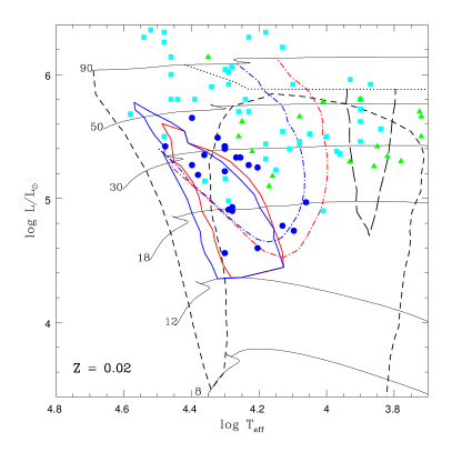
Figure 1: Instability boundaries of various modes with selected evolutionary tracks. Black short-dashed and long-dashed lines are for low-order and high-oder (radial and nonradial) p-modes, respectively. Dotted line is the boundary above which monotonously unstable modes present. Red and blue solid lines are for nonradial g-modes with $\ell=1$ and $\ell=2$, respectively. Dash-dotted lines are for oscillatory convection modes (red line for $\ell=1$, blue line for $\ell=2$) indicating the boundaries of the region where the ratio of the photospheric to the maximum amplitude in the interior is larger than 0.2. The number written at the start of each evolutionary track indicates the initial mass $M_{i}$ in solar mass units. Wind mass loss included for the evolutionary models with $M_{i}\geq 30M_{\odot}$ based on Vink et al. (2001). Also shown are positions of super-giant variable stars; variable B-type supergiants (blue dots Lefever et al., 2007), S Dor variables (cyan squares van Genderen, 2001), and $\alpha$ Cyg variables (red triangles , van Leeuwen, et al.1998; van Genderen & Sterken, 2002).

Fig. 1 shows various instability boundaries (visibility boundaries for oscillatory convection modes) obtained in this paper and selected evolutionary tracks for a standard composition of $(X,Z)=(0.7,0.02)$. For comparison, positions of periodic and semi-periodic supergiant variables are plotted from various sources of the observational data. Interestingly, most of those variable supergiants reside in the unstable regions.

The short-dashed line in Fig. 1 shows the instability boundary of low-order radial and nonradial p-mode oscillations. In the long nearly vertical region of $4.6\ga\log T_{\rm eff}\ga 4.3$, the kappa-mechanism at the Fe opacity bump excites low-order modes, which correspond to $\beta$ Cep variables (, Kiriakidis et al.1992; Moskalik & Dziembowski, 1992; Pamyatnykh, 1999).

The instability boundary bends and becomes horizontal due to strange mode instability (, Kiriakidis et al.1993; Glatzel, 1994; Saio, et al., 1998) which occurs when the luminosity to mass ratio is sufficiently high ($L/M\ga 10^{4}L_{\odot}/M_{\odot}$) and radiation pressure is dominant at least locally in the envelope. The instability boundary is essentially the same as that obtained by (Kiriakidis et al.1993) for $Z=0.02$. In the hottest part, the strange modes are associated with the Fe opacity peak, while in relatively cooler part the contribution from the opacity peak at the second helium ionization becomes important.

The vertical part around $\log T_{\rm eff}\sim 3.8$ is the well known blue edge of the Cepheid instability strip.

A narrow vertical region indicated by a long-dashed line around $\log T_{\rm eff}\sim 3.8-3.9$ in Fig. 1 indicates the excitation of relatively high order radial and nonradial modes due the strange mode instability associated with the hydrogen ionization zone. We will discuss these modes in §3.3.

Monotonously unstable modes exist above the dotted line in the most luminous part of Fig. 1, which will be discussed in §3.2.

In the regions surrounded by blue and red solid lines, nonradial g-modes are excited by the Fe opacity bump; red and blue lines for $\ell=1$ and $\ell=2$ modes, respectively. Those g-modes can be excited even in the post-main-sequence models if the mass exceeds $12M_{\odot}$, because a convection zone above the hydrogen burning shell can block some g-modes from penetrating to the core.

3.1 Oscillatory convection modes

Figure 2: Runs of radial displacements (bottom panels) and kinetic energy distributions (top panels) as function of fractional radius ($r/R$) for selected oscillatory convection modes of $\ell=1$ in two supergiant models with different effective temperatures but with the same initial mass of $60M_{\odot}$. Also shown are runs of temperature and the ratios of radiation to total flux ($F_{\rm rad}/F_{\rm tot}$) and radiation pressure to total pressure ($1-\beta$). The numbers in parentheses are the real and imaginary parts of eigenfrequencies normalized by $\sqrt{GM/R^{3}}$.

The dash-dotted lines in Fig. 1 are the ranges where oscillatory convection modes would be observable; red and blue lines are for $\ell=1$ and $\ell=2$ modes, respectively. The observability is determined based on the ratio between the photospheric amplitude and the maximum amplitude in the interior, which is discussed below.

Fig. 2 shows distributions of radial displacements ($\xi_{r}/r$, bottom panels) and kinetic energy density ($de_{k}/dr$, top panels) of oscillatory convection modes of $\ell=1$ in two (hot and relatively cool) models from the $M_{i}=60M_{\odot}$ ($Z=0.02$) evolutionary sequence. Two convection modes for each model are shown with selected physical quantities. A convection zone can be recognized as a zone where the ratio of radiative to total energy flux is less than unity;i.e., $F_{\rm rad}/F_{\rm tot}<1$. The Fe-convection zone occurring in a temperature range of $5.4\ga\log T\ga 4.9$ has a considerable thickness but contains very small mass ($\la 10^{-3}M_{\odot}$ for the hotter model, and $\sim 4\times 10^{-3}M_{\odot}$ for the cooler model). Because the gas density is very low in the envelope of a massive star, the convective flux is less than 50% of the total energy flux. In addition, the low density makes the gas pressure much smaller than the radiation pressure; i.e., $\beta\ll 1$ with $\beta$ being the ratio of gas to total pressure.

Two modes shown for each model in Fig. 2 are the two shortest period convection modes that are most likely observable; i.e., ratios of the photospheric amplitude to the maximum amplitude in the interior are largest (see also Fig. 3). The numbers in parentheses in the bottom panels of Fig. 2 are normalized (by $\sqrt{GM/R^{3}}$) complex eigenfrequencies; the real part represents oscillation frequency, and imaginary part growth or damping rate. When the imaginary part is negative the oscillation grows. The eigenfrequencies shown in Fig. 2 indicate that the growth times are comparable to the periods. The periods are comparable to the periods of g-modes.

The kinetic energy of the oscillatory convection modes is confined to and slightly above the convection zone in the hotter model, while it is well confined to the convection zone in the cooler model. For the convection modes shown in this figure, the oscillation amplitude at the stellar surface is comparable to that in the convective zone, indicating those modes are very likely observable.

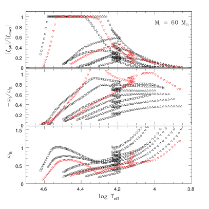
Figure 3: Some properties of oscillatory convection modes versus effective temperature along the evolutionary track of $M_{i}=60M_{\odot}$ with $Z=0.02$; bottom panel: Real part of normalized frequencies; middle panel: growth rate; top panel:the ratio of the amplitude of the photosphere to the maximum amplitude. Triangles and squares are for $\ell=1$ and $\ell=2$, respectively. Red inverted triangles are for $\ell=1$ modes in models calculated with a mixing-length of one pressure scale-height.

Since oscillatory convection modes have short growth-times, we expect that they have substantial amplitudes in the convection zone. For such a mode to be observable, however, the amplitude at the stellar surface should be, at least, considerable relative to the amplitude in the convection zone. We assume that the possibility of detecting these convection modes can be measured by the ratio of the photospheric amplitude to the maximum amplitude in the interior. The ratio differs for different modes in a model and changes as the stellar parameters change. The top panel of Fig. 3 shows variations of the ratio as a function of effective temperature along the evolutionary track of $M_{i}=60M_{\odot}$ for a few convection modes of $\ell=1$ (triangles) and $\ell=2$ (squares). This figure shows that although many convection modes exist in a model, only one or two highest-frequency modes (for each $\ell$) have large values of the amplitude ratio and hence are potentially observable. Generally, the amplitude ratio of each mode has a broad peak as a function of effective temperature, and the peak value tends to be larger for a mode with larger frequency (bottom panel) and larger growth rate (middle panel). In other words, the visibility is highest for largest frequency modes with highest growth rates in a certain effective temperature range ($4.2\la\log T_{\rm eff}\la 4.6$ for the $M_{i}=60M_{\odot}$ models).

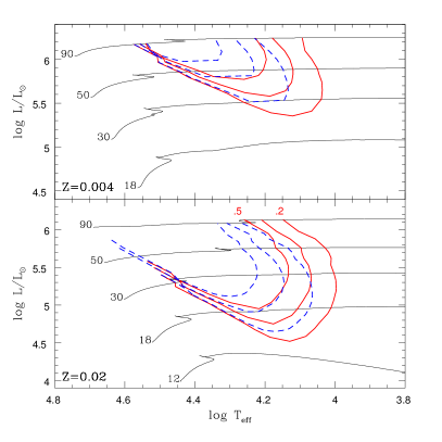
Figure 4: Contours of $0.5,1/3$ and $0.2$ for the ratio of the amplitude at the photosphere to the maximum amplitude in the interior. Solid and dash-dotted lines are for $\ell=1$ and $\ell=2$ modes, respectively. The bottom panel is for normal metallicity of $Z=0.02$ and the top panel for a metal-poor composition of $Z=0.004$.

Fig. 4 shows contours of the amplitude ratio for the most visible convection modes for $\ell=1$ (solid lines) and $\ell=2$ (dashed lines). Generally, the visibility of the oscillatory convection modes is better in more luminous and hotter models. We assume in this paper that these modes would be well visible when the ratio exceeds $0.2$. The contours for the ratio of $0.2$ are shown in Fig. 1.

The top panel of Fig. 4 shows the contours obtained for models with $(X,Z)=(0.716,0.004)$. Since the opacity is much lower than that for the case of $Z=0.02$, the convection zone around the Fe opacity peak is less extensive. Nonetheless, observable oscillatory convection modes with low degree $\ell=1,2$ persist, although the contour for a value of the amplitude ratio shifts upward by $\Delta\log L\approx 0.8$ as compared to the case of the standard composition. This indicates that oscillatory convection modes can cause observable variations even in the SMC if the stars are luminous enough.

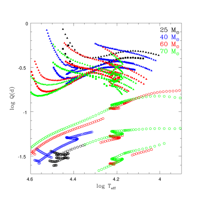
Figure 5: Q-values of convection modes (filled triangles for $\ell=1$, filled squares for $\ell=2$) and excited radial modes (open circles) versus effective temperatures along the evolutionary tracks of $M_{i}=25,40,60$ and $70M_{\odot}$.

The growth rates of the oscillatory convection modes (middle panel, Fig.3) are very high, especially in relatively cooler models; they tend to decrease as $T_{\rm eff}$ increases. The reason is probably that in hotter models kinetic energy distribution shifts outward and hence a large fraction of the kinetic energy resides above the convective zone boundary losing the driving.

It has been thought that the pulsation modes with the highest growth rates are associated with strange modes (eg. Gautschy & Glatzel, 1990b; Saio, et al., 1998). The growth rates of the convection modes are even larger than those of radial strange modes in massive stars (Glatzel & Kiriakidis, 1993; , Kiriakidis et al.1993). The oscillation frequencies of convection modes lie in the g-mode range as seen in the bottom panel of Fig. 3, indicating the periods of convection modes are longer than radial modes.

Fig. 5 shows Q-values of convection modes with the amplitude ratio larger than $0.2$ (filled symbols) compared with excited radial modes (open circles) for some selected mass models, where the Q-value is defined as $\Pi\sqrt{\overline{\rho}/\overline{\rho}_{\odot}}$ with $\Pi$ and $\overline{\rho}$ being, respectively, pulsation period and mean density (see e.g. Cox, 1980). The Q-value of a convection mode decreases rapidly as the effective temperature decreases in the hottest and the coolest $T_{\rm eff}$ ranges, while it changes little in the intermediate range of effective temperature. At a given effective temperature, Q-values of oscillatory convection modes tend to be smaller in more massive models.

In very massive ($M_{i}=60,70M_{\odot}$) models, radial pulsations are excited even in cooler ($\log T_{\rm eff}\la 4.2$) models due to mainly the strange mode effect that works around the second He ionization zone (Glatzel & Kiriakidis, 1993; , Kiriakidis et al.1993). The Q-values of these strange modes increases as the effective temperature decreases; i.e., as the depth of the He II ionization zone increases. Fig. 5 indicates that periods of oscillatory convection modes are much longer than those of radial pulsations in hotter models, although in cooler and massive models the differences are not very large. Lamers et al. (1998) found that the periods of microvariations of LBVs are orders of magnitudes longer than those predicted for strange modes by (Kiriakidis et al.1993). This indicates that oscillatory convection modes would be responsible for long-period microvariations in LBVs (see §4 below).

Red inverted triangles in Fig. 3 present the property of oscillatory convection modes of $\ell=1$ in models calculated with a mixing-length of one pressure scale-height rather than $1.5$ pressure scale-hight adopted in standard models. A smaller mixing-length makes the super-adiabatic temperature gradient in the Fe-convection zone larger. In the models with the smaller mixing-length, real parts of eigenfrequencies of oscillatory convection modes tend to be smaller, and the amplitude tends to be slightly more confined to the convection zone. Fortunately, the qualitative property of the oscillatory convection modes is insensitive to the mixing-length parameter.

3.2 Monotonously unstable mode

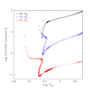
Figure 6: Growth-time versus effective temperature for monotonously unstable modes in models with $M_{i}=60M_{\odot},70M_{\odot}$ and $90M_{\odot}$.

In very massive models ($M_{i}\geq 60M_{\odot}$) a monotonously unstable radial mode (with a purely imaginary eigenfrequency) is found in the range on the HR diagram indicated by a dotted line in Fig. 1. Fig. 6 shows growth time as a function of effective temperature for those unstable modes in models with different initial masses. The growth times tend to be shorter for more massive stars, ranging from a month to a hundred years, which are much faster than the evolutionary change. It is interesting to note that the range of the growth times includes the timescales of S Dor (SD)-phase (van Genderen, 2001). To the author’s knowledge, the presence of monotonously unstable modes in very massive stars was not known before. The presence was unrecognized in the non-linear radial pulsation analyses performed before by various authors, probably because the monotonously unstable mode was concealed by the more fast growing strange mode pulsations.

Figure 7: The amplitude of displacement ($|\xi/r|$) and kinetic energy distribution ($de_{k}/dr$) and selected physical quantities as functions of the fractional radius ($r/R$) for a model with $M_{i}=70M_{\odot}$, where $\kappa$ is opacity, and other quantities are the same as in Fig. 2.

Amplitude and kinetic energy distribution of the monotonously unstable mode in a model with $M_{i}=70M_{\odot}$ are shown in Fig. 7. The amplitude and kinetic energy have a peak around the bottom of the convective zone generated by the Fe-opacity peak; in this model the convective zone ranges from $r/R=0.20$ to $0.595$. Although, the kinetic energy, as well as amplitude, is confined around the bottom of the convection zone, the amplitude, after attaining a minimum at $r/R\approx 0.45$, gradually increases toward the surface above the convection zone. In a substantial range in this model the ratio of the gas to radiation pressure is very small (i.e., $\beta\ll 1$). Then,

$${L_{\rm rad}\over L_{\rm Edd}}\approx(1-\beta)\approx 1,$$ (1)

where $L_{\rm rad}$ is radiative luminosity and $L_{\rm Edd}$ the local Eddington luminosity defined as

$$L_{\rm Edd}\equiv 4\pi cGM_{r}/\kappa$$ (2)

with $c$ being the velocity of light and $M_{r}$ the mass within the sphere of radius $r$. This suggests that the monotonously unstable mode arises because the radiative luminosity is very close to the local Eddington luminosity in a substantial range of the envelope.

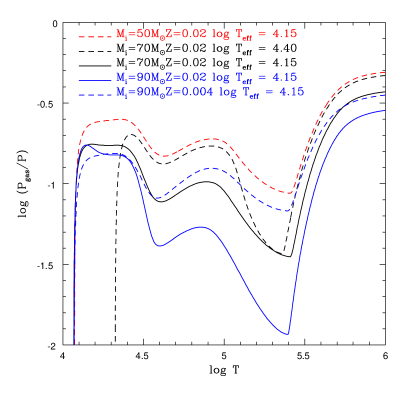
Figure 8: Distribution of the ratio $P_{\rm gas}/P$ ($\equiv\beta$) in the interior of selected models. Solid lines are used for the models which has a monotonously unstable mode, while broken lines for the models having none.

Fig. 8 shows the distribution of $\beta$ in selected models, where solid lines are used for models which have a monotonously unstable mode, while dashed lines are for models without it. There are two minima of $\beta$ at $\log T\approx 5.4$ (Fe opacity peak) and at $\log T\approx 4.6$ (He II ionization). Apparently, $\beta$ must be well below 0.1 in a range including the both opacity peaks for a monotonously unstable mode to appear. Note that the hotter model of $70M_{\odot}$ (black dashed line) has a distribution of $\beta$ around $5.2\la\log T\la 5.4$ similar to that of the cooler model (black solid line), but $\beta$ in the range $4.5\la\log T\la 5$ is significantly higher than that in the cooler model, which inhibits a monotonously unstable mode in the hotter model. With a low-metal abundance of $Z=0.004$ no monotonously unstable mode is found even in models of $M_{i}=90M_{\odot}$. The reason is obvious from the blue dashed line in Fig. 8; $\beta$ at the Fe opacity peak is substantially larger, although a further increase in mass seems to cause monotonously unstable modes.

The presence of such a monotonously unstable mode probably corresponds to the presence of an optically thick wind as discussed by Kato & Iben (1992) and Nugis & Lamers (2002) for WR stars. It is known that optically thick winds also occur in nova models. Kato & Hachisu (2009) have shown that for non-extreme nova cases both static models and models with winds are possible. The presence of a monotonously unstable mode in a massive evolutionary model might indicate that the static model transits to a model with an optically thick wind.

It is interesting to note that the boundary in the HR diagram for the presence of monotonously unstable modes (dotted line in Fig. 1) roughly coincides with the Humphreys-Davidson (HD) limit (Humphreys & Davidson, 1979); this may suggest the HD limit to be related to the presence of optically thick winds.

3.3 High-oder modes excited at H ionization zone

In the narrow vertical region around $\log T_{\rm eff}\sim 3.9$ seen in Fig. 1, relatively high order ($n\sim 6-10$) radial as well as nonradial modes are excited at the hydrogen ionization zone at $\log T\approx 4$. Since the normalized frequency of the excited mode increases as the effective temperature decreases, the red-edge is formed where the frequency exceeds the critical frequency given as ${1\over 2}\sqrt{\Gamma_{1}R/H_{p}}$ with the pressure scale height $H_{p}$ and $\Gamma_{1}\equiv(d\ln P/d\ln\rho)_{\rm ad}$. (If the frequency exceeds the critical frequency, the pulsation is not reflected at the outer boundary and is expected to be dissipated in the outermost layers.)

Figure 9: Amplitude distribution and work curve (top panel) for an excited 9th-order radial pulsation. Some physical quantities are shown in the bottom panel.

Fig. 9 shows the amplitude distribution and the work curve for a high-order radial mode excited in a model relatively close to the blue edge. Obviously the excitation occurs at $\log T\approx 4$, in the hydrogen ionization zone. The amplitude of the mode is extremely confined to the surface layers, where the radiation pressure is much larger than the gas pressure. Since unstable modes of this type are present even in the non-adiabatic reversible (NAR; Gautschy & Glatzel, 1990b) approximation where thermal-time is artificially set to be zero, we can identify such a mode as a strange mode trapped above the opacity peak of the hydrogen ionization. A similar mode with a similar frequency is excited for $\ell=1$ and $\ell=2$. These excited nonradial modes probably correspond to the trapped modes discussed in Gautschy (2009). In addition to the trapped modes Gautschy (2009) found several untrapped modes to be excited around the trapped mode frequency, by using the Riccati-shooting method discussed in Gautschy & Glatzel (1990a). The present study using a finite difference method, however, could not find those untrapped modes. According to Gautschy (2009) those modes have many nodes with considerable amplitude in the deep interior around $r/R\sim 10^{-2}$. The finite difference code even with $\sim 10^{4}$ grid points seems ineffective to find such untrapped modes.

4 Comparison with observed periods

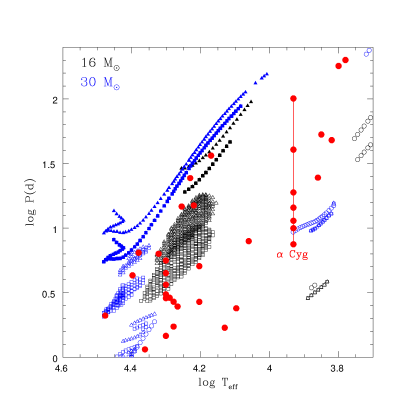
Figure 10: Periods of radial and nonradial modes excited in $16$ and $30M_{\odot}$ models are compared with observed periods of relatively less luminous ($\log L/L_{\odot}\leq 5.5$) supergiants (large dots) which consists of periodic B stars from Lefever et al. (2007) and relatively cooler less luminous $\alpha$ Cyg variables from (van Leeuwen, et al.1998) and van Genderen & Sterken (2002). The periods of $\alpha$ Cyg itself are adopted from Lucy (1976), while the effective temperature from Schiller & Przybilla (2008). Triangles and squares correspond to $\ell=1$ and $\ell=2$, respectively. Filled triangle and squares are convection modes for which the amplitude ratios (see §3.1) are larger than 0.2. Open circles are radial modes. Swarms of $\ell=1,2$ modes in a range of $4.35\ga\log T_{\rm eff}\ga 4.15$ for $16M_{\odot}$ and in a range of $4.5\ga\log T_{\rm eff}\ga 4.35$ for $30M_{\odot}$ are high-order g-modes (i.e., SPBsg-type oscillations).

Fig. 10 compares periods of radial and nonradial modes excited in $16M_{\odot}$ and $30M_{\odot}$ models with observed periods of relatively less luminous ($\log L/L_{\odot}<5.5$) supergiant variables as function of $T_{\rm eff}$. Those variables consist of most of the periodic B stars analyzed by Lefever et al. (2007), and relatively cooler $\alpha$-Cygni variables including $\alpha$ Cyg itself. Most of the periods of the hotter ($\log T_{\rm eff}\ga 4.15$) less luminous supergiants seem consistent with oscillatory convection modes, SPB-type g-modes (SPBsg), or p-modes.

Relatively cool ($\log T_{\rm eff}\la 3.95$) stars in Fig. 10 are less luminous $\alpha$-Cygni variables. They lie in the $T_{\rm eff}$ range where high-order p-modes are excited (Fig. 1), although most of the periods are longer than those of high-order p-modes. Probably they are pulsating in g-modes excited in a similar range of $T_{\rm eff}$ as found by Gautschy (2009), who found that g-modes having periods of ranging from about 10 to 20 days are excited at the hydrogen ionization zone, although a large fraction of their kinetic energy resides in the deep interior.

No modes can be assigned to the three stars in a range of $4.15\ga\log T_{\rm eff}\ga 4.05$ in Fig. 10, which are the coolest members in the data from Lefever et al. (2007) (Fig.1). The cause of the oscillations in these stars is not clear.

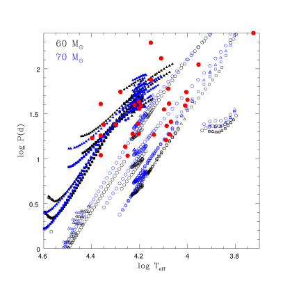
Figure 11: Periods of radial and nonradial modes excited in high mass models of $M_{i}=60M_{\odot}$ and $70M_{\odot}$ with $Z=0.02$ are compared with observed periods of luminous ($\log L/L_{\odot}\geq 5.5$) supergiants (red dots) which consists of microvariations of LBVs from Lamers et al. (1998) and luminous $\alpha$ Cyg variables from (van Leeuwen, et al.1998) and van Genderen & Sterken (2002). Symbols for theoretical periods have the same meanings as in Fig. 10.

Fig. 11 compares periods of radial and nonradial modes excited in higher mass models of $M_{i}=60$ and $70M_{\odot}$ with observed ones for microvariations in luminous ($\log L/L\geq 5.5$) supergiants which consist of LBVs and luminous $\alpha$ Cyg variables. In these massive stars, radial and nonradial strange modes are excited (open symbols), and oscillatory convection modes (filled triangles and squares) are likely observable (the amplitude ratio is larger than 0.2) in a wide range of $T_{\rm eff}$, while SPB-type g-modes are not excited.

Fig. 11 indicates that most of the periods of microvariations of LBVs and luminous $\alpha$ Cyg variables are consistent with the periods of oscillatory convection modes and strange modes.

The comparisons between observed and theoretical periods in Figs. 10 and  11 indicate that $\alpha$-Cygni variables are inhomogeneous. Luminous ones are similar to the microvariations of LBVs which are identified as oscillatory convection modes or strange modes, while less luminous cooler ones, including $\alpha$ Cyg itself, seem to be g-modes (and possibly including high-order strange modes) excited at the hydrogen ionization zone.

5 Low metallicity cases

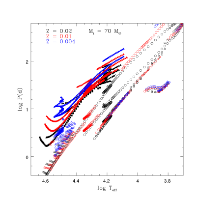
Figure 12: Periods of radial and nonradial oscillations excited in models with different heavy element abundances are compared. The symbols for the excited modes are the same as in Fig. 10.

Since there are some LBVs and $\alpha$ Cyg variables in SMC, it would be useful to discuss the results for low metal abundances. Fig. 12 compares periods of radial and nonradial modes excited in models with $M_{i}=70M_{\odot}$ having different metal abundances. The difference between the cases of $Z=0.02$ and $Z=0.01$ is small, while the case of $Z=0.004$ is significantly different from the former cases. Because of the Fe-opacity peak being reduced, strange mode instability for low-order radial and nonradial modes are reduced significantly for the $Z=0.004$ case, while the excitation of SPBsg-type g-modes seems to be enhanced in the lowest metallicity case (the reason is not clear).

It is interesting to note that even for the low metallicity of $Z=0.004$ oscillatory convection modes still seem to be observable in a considerable range of $T_{\rm eff}$ (see also Fig. 4).

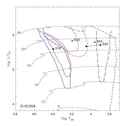
Figure 13: The same as Fig. 1 but for a metal-poor composition of $(X,Z)=(0.716,004)$. Also plotted are some S Dor variables (van Genderen, 2001) and $\alpha$ Cyg variables (, van Leeuwen, et al.1998) in SMC.

Fig. 13 is the same as Fig. 1 but for $Z=0.004$; i.e., shows instability ranges for radial and nonradial modes and observable ranges for oscillatory convection modes in the HR diagram. Compared to the case of $Z=0.02$ (Fig. 1), the instability region for low-order radial and nonradial p-modes (i.e., $\beta$ Cep instability strip) has disappeared completely. The instability boundary for the low-order strange mode instability has shifted upward considerably, which agrees with the result of (Kiriakidis et al.1993).

On the other hand, less affected are the SPBsg-type g-mode instability regions and the observable region of oscillatory convection modes. The instability region for high-order modes in $3.95\ga\log T_{\rm eff}\ga 3.8$ is not affected because they are excited at hydrogen ionization zone. Positions of some LBVs (S Dor variables) and $\alpha$ Cyg variables in SMC are also plotted in Fig. 13. Fig. 14 compares quasi-periods of the microvariations of those stars with theoretical periods predicted for metal poor models with initial masses ranging from $M_{i}=30$ to $90M_{\odot}$.

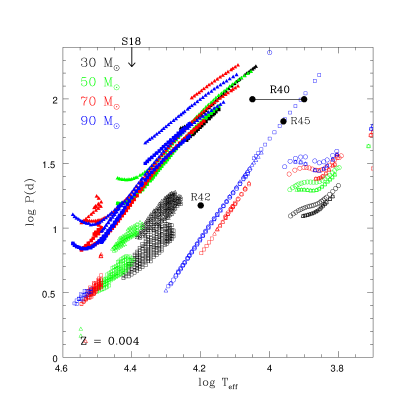
Figure 14: Periods of excited modes in metal-poor models ($Z=0.004$) of $M_{i}=30,50,70$, and $90M_{\odot}$ as function of $T_{\rm eff}$ are compared with observed periods of microvariations of LBVs and $\alpha$ Cyg variables in SMC. Symbols for theoretical periods have the same meanings as in Fig. 10.

In contrast to the Galactic and LMC cases, oscillatory convection modes seem to be responsible for none of the SMC stars shown in these figures. Fig. 14 seems to indicate that periods of low-order strange modes are comparable with those of the microvariations of R40 and R45 (and probably R42). For the strange mode interpretation to be true, the initial mass must be greater than $\sim 80M_{\odot}$. Fig. 13, however, indicates the initial mass of these stars to be $40-50M_{\odot}$; i.e., the luminosities of these stars seem too low at least by a factor of two. Therefore, the mode identification for the microvariations of R40, R42 and R45 is unclear.

For S18, an $\alpha$ Cyg variable in the SMC, only the effective temperature is indicated in Fig. 14 because the quasi-periods of its variability are uncertain. van Genderen & Sterken (2002) found three types of variations on timescales of a few years, $\sim 150$ days, and a few days. Figs. 13 and 14 indicate the shortest timescale variation to correspond to the SPBsg type g-modes. For the longer-periods variations, however, no excited oscillation modes can be assigned.

6 Conclusions

The stability of radial and nonradial modes in massive stars ($90\geq M_{i}/M_{\odot}\geq 8$) was investigated. The $\kappa$-mechanism associated with the Fe-opacity bump at $T\sim 2\times 10^{5}$K excites low-order radial and nonradial p-modes in main-sequence and post-main-sequence models ($\beta$ Cep instability strip) and low-degree high radial order g-modes in post-main sequence models (supergiant SPB stars; SPBsg ). Interestingly, it is found that under a low-metal composition of $Z=0.004$, the SPBsg instability region still remains, while the $\beta$ Cep instability strip disappears.

In luminous models with $L/M\ga 10^{4}L_{\odot}/M_{\odot}$ (for $Z=0.02)$ strange mode instability occurs associated with opacity peaks due to Fe and He II ionizations. For the metal-poor composition $Z=0.004$ strange mode instability appears only in more luminous models.

In a narrow strip of $3.95\ga\log T_{\rm eff}\ga 3.85$, high-order radial and nonradial pulsations are excited at the hydrogen-ionization zone. The pulsation amplitude is strongly confined to the outermost layers.

Low-$\ell$ oscillatory convection modes associated with the Fe convection zones in massive stars are found. They are likely observable in sufficiently luminous models in a considerable range of effective temperature. The oscillatory convection modes tend to have growth times comparable with the periods. Their periods are longer than those of strange modes or SPBsg-type g-modes, and are comparable to those of long-period microvariations of LBVs and luminous $\alpha$ Cyg variables. Rapid growth rates of the oscillatory convection modes are consistent with the presence of irregularities in the microvariations.

In addition to the oscillation modes, a monotonously unstable mode is found in luminous models with $\log L\ga 5.9$ and $\log T_{\rm eff}\la 4.3$. The boundary in the HR diagram for the presence of the monotonously unstable mode roughly coincides with the HD limit. The growth rate is more than hundred times faster than the stellar evolution rate. It probably suggests the presence of an optically thick wind in such a luminous star.

Finally, it should be noted that in the present stability analysis the effect of stellar winds is not included in the outer boundary condition. In the future, we have to clarify how the stellar wind affects the stability of oscillations of massive stars.

References

- Aerts et al. (2010) Aerts C., Lefever K., Baglin A., Degroote P., Oreiro R., Vucković M., Smolders K., Acke B., Verhoelst T., Desmet M., et al., 2010, A&A, 513, L11
- Cantiello et al. (2009) Cantiello M., Langer N., Brott I., de Koter A., Shore S.N., Vink J.S., Voegler A., Lennon D.J., Yoon S.-C., 2009, A&A, 499, 279
- (3) Chernigovski S., Grott M., Glatzel W., 2004, MNRAS, 348, 192
- Cox (1980) Cox J.P., 1980 Theory of Stellar Pulsation (Princeton Univ. Press)
- Degroote et al. (2010) Degroote P., Briquet M., Auvergne M., Simón-Díaz S., Aerts C., Noels A., Rainer M., et al., 2010, A&A, 519, A38
- Dorfi & Gautschy (2000) Dorfi E.A., Gautschy A., 2000, ApJ, 545, 982
- Dziembowski & Sławińska (2005) Dziembowski W.A., Sławińska J., 2005, AcA, 55, 195
- Fadeyev (2010) Fadeyev Yu.A., 2010, Ast.Let., 36, 362
- Gautschy (2009) Gautschy A., 2009, A&A, 498, 273
- Gautschy & Glatzel (1990a) Gautschy A., Glatzel 1990a, MNRAS, 245, 154
- Gautschy & Glatzel (1990b) Gautschy A., Glatzel 1990b, MNRAS, 245, 597
- Glatzel (1994) Glatzel W., 1994, MNRAS, 271, 66
- Glatzel & Kiriakidis (1993) Glatzel W., Kiriakidis M., 1993, MNRAS, 263, 375
- Godart et al. (2009) Godart M., Noels A., Dupret M.-A., Lebreton Y. 2009, MNRAS, 396, 1833
- (15) Grott M., Chernigovski S., Glatzel W., 2005, MNRAS, 360, 1532
- Humphreys & Davidson (1979) Humphreys R.M., Davidson K., 1979, ApJ, 232, 409
- Humphreys & Davidson (1994) Humphreys R.M., Davidson K., 1994, PASP, 106, 704
- Iglesias & Rogers (1996) Iglesias C.A., Rogers R.J., 1996, ApJ, 464, 943
- Kato & Iben (1992) Kato M., Iben I.Jr, 1992, ApJ, 394, 305
- Kato & Hachisu (2009) Kato M., Hachisu I., 2009, ApJ, 699, 1293
- (21) Kiriakidis M., El Eid M.F., Glatzel W., 1992, MNRAS, 255, 1p
- (22) Kiriakidis M., Fricke K.J., Glatzel W., 1993, MNRAS, 264, 50
- Lamers et al. (1998) Lamers H.J.G.L.M., Bastiaanse M.V., Aerts C., Spoon H.W.W., 1998, A&A, 335, 605
- Lefever et al. (2007) Lefever K., Puls J., Aerts C., 2007, A&A, 463, 1093
- Lucy (1976) Lucy L.B., 1976, ApJ, 206, 499
- Moskalik & Dziembowski (1992) Moskalik P., Dziembowski W.A., 1992 A&A, 256, L5
- Nugis & Lamers (2002) Nugis T., Lamers H.J.G.L.M., 2002, A&A, 389, 162
- Pamyatnykh (1999) Pamyatnykh A.A., 1999, Acta Astron, 49, 119
- Rogers & Iglesias (1992) Rogers, F.J., Iglesias, C.A., 1992, ApJS, 79, 507
- Saio & Cox (1980) Saio H., Cox J.P., 1980, ApJ, 236, 549
- Saio, et al. ( 1998) Saio H., Baker N.H., Gautschy A., 1998, MNRAS, 294, 622
- Saio, et al. (2006) Saio H., Kuschnig R., Gautschy A., Cameron C., Walker G.A.H., Matthews J.M., et al., 2006, ApJ, 650, 1111
- (33) Saio H., Winget D.E., Robinson E.L., 1983, ApJ, 265, 982
- Shibahashi & Osaki (1981) Shibahashi H., Osaki Y., 1981, PASJ, 33, 427
- Schiller & Przybilla (2008) Schiller F., Przybilla N., 2008, A&A, 479, 849
- van Genderen (2001) van Genderen A.M., 2001, A&A, 366, 508
- van Genderen & Sterken (2002) van Genderen A.M., Sterken, C., 2002, A&A, 386, 926 van Genderen A.M., Sterken C., Jones A.F., 2004, A&A, 419, 667
- (38) van Leeuwen F., van Genderen A.M., Zegelaar, I., 1998, A&AS, 128, 117
- Vink et al. (2001) Vink J.S., de Koter A., Lamers H.J.G.L.M., 2001, A&A, 369, 574
- Waelkens, et al. (1998) Waelkens C., Aerts C., Kestens E., Grenon M., Eyer L., 1998, A&A, 330, 215