solving optimal dividend problems via phase-type fitting approximation of scale functions

Abstract.

The optimal dividend problem by De Finetti, (1957) has been recently generalized to the spectrally negative Lévy model where the implementation of optimal strategies draws upon the computation of scale functions and their derivatives. This paper proposes a phase-type fitting approximation of the optimal strategy. We consider spectrally negative Lévy processes with phase-type jumps as well as meromorphic Lévy processes (Kuznetsov et al., 2010a, ), and use their scale functions to approximate the scale function for a general spectrally negative Lévy process. We obtain analytically the convergence results and illustrate numerically the effectiveness of the approximation methods using examples with the spectrally negative Lévy process with i.i.d. Weibull-distributed jumps, the $\beta$-family and CGMY process.

Key words: De Finetti’s dividend problem; phase-type models; Meromorphic Lévy processes; Spectrally negative Lévy processes; Scale functions
JEL Classification: G22, D81, C61
Mathematics Subject Classification (2000) : Primary: 93E20 Secondary: 60G51

1. Introduction

In the optimal dividend problem, an insurance company wants to maximize the cumulative amount of dividends paid out to its beneficiaries until the time of ruin. The original problem by De Finetti, (1957) considered a discrete-time case by modeling the surplus by a random walk. It has been later extended to the continuous-time diffusion model (Jeanblanc and Shiryaev, , 1995; Asmussen and Taksar, , 1997; Gerber and Shiu, , 2004) and to the Cramér-Lundberg model (Gerber, , 1969; Azcue and Muler, , 2005). It was recently generalized to the spectrally negative Lévy model by Avram et al., (2007) and Kyprianou and Palmowski, (2007) where the surplus is a general Lévy process with only negative jumps.

The implementation of the optimal strategies in the spectrally negative Lévy model draws upon the computation of the so-called scale function. Avram et al., (2007) first obtained the expected value under a barrier strategy in terms of the scale function. Loeffen, (2008) then showed that a barrier strategy is indeed optimal under a suitable condition. The scale function also plays great roles in its extensions with transaction costs and additional terminal values at ruin. See Loeffen, 2009a ; Loeffen, 2009b and Loeffen and Renaud, (2010).

Despite these advances, a major obstacle still remains in putting in practice the above-mentioned results because scale functions are in general known only up to their Laplace transforms. The implementation is even harder for the optimal dividend problem because it requires the first derivative of the scale function. One can in principle approximate the scale function and its derivative via the numerical Laplace inversion as discussed in Surya, (2008). However, the method is only heuristic and one cannot determine the accuracy of the approximation. Moreover, the derivative of the scale function tends to explode in the neighborhood of zero, and therefore the error is expected to be large near zero. For these reasons, there is a clear need of new approximation methods that work for any spectrally negative Lévy process.

As a new tool to overcome these problems, this paper proposes a phase-type fitting approach to approximate the scale functions as well as the solutions to the optimal dividend problem and its extensions. We obtain the scale functions of spectrally negative Lévy processes with phase-type jumps and those in the M-class (meromorphic Lévy processes), and apply these for a general spectrally negative Lévy model.

We first consider the class of spectrally negative Lévy processes with phase-type jumps. Consider a continuous-time Markov chain with some initial distribution and state space consisting of a single absorbing state and a finite number of transient states. The phase-type distribution is the distribution of the time to absorption. It is known that the class of phase-type distributions is dense in the class of all positive-valued distributions. We obtain the scale functions for these processes and show that they can approximate the scale function of a general spectrally negative Lévy process arbitrarily closely.

The phase-type fitting approach has mainly three advantages. First, thanks to the smoothness and monotonicity properties of scale functions as proved by, for example, Chan et al., (2009) and Loeffen, (2008), the approximation can be applied also to its derivative. Second, the Laplace transform of the phase-type distribution has an explicit expression and hence can avoid the error caused while approximating the Laplace transform for a general jump distribution. This type of errors tends to occur in other approximation methods such as Surya, (2008). Third, the phase-type fitting approach enjoys a variety of fitting algorithms. See, for example, Asmussen, (1996), Bladt et al., (2003) and Feldmann and Whitt, (1998). The fitting can be applied also to empirical data and this is another major advantage. In the first half of our numerical results, we use the results by Feldmann and Whitt, (1998) and consider the case with a Brownian motion plus a compound Poisson with Weibull-distributed jumps.

We also consider meromorphic Lévy processes (Kuznetsov et al., 2010a, ), which generalizes a number of recently-discovered Lévy processes such as Lamperti-stable processes (Caballero and Chaumont, , 2006; Chaumont et al., , 2009), hypergeometric processes (Kyprianou, , 2010; Kuznetsov et al., 2010b, ) and processes in the $\beta$- and $\Theta$-families (Kuznetsov, 2009a, ; Kuznetsov, 2009b, ). The spectrally negative versions of these processes commonly have Lévy measures in the form

(1.1) $$\nu({\rm d}z)=\left[\sum_{i=1}^{\infty}\alpha_{i}\eta_{i}e^{-\eta_{i}|z|}1_{\{z<0\}}\right]{\rm d}z,\quad z\in\mathbb{R},$$

which can be seen as an extension of the hyperexponential density and as a “discrete version” of the completely monotone density.

The reason we consider the Lévy measure above is that it can approximate efficiently any Lévy measure with a completely monotone density. Furthermore, if the Lévy measure is completely monotone, the barrier-strategy is guaranteed to be optimal for the dividend problem (Loeffen, , 2008). The class of Lévy measures with completely monotone densities is rich. It enables us to model compound-Poisson-type jumps with long-tailed distributions such as the Pareto, Weibull and gamma distributions; see Feldmann and Whitt, (1998). It further allows us to construct many of recently-introduced Lévy processes such as variance gamma processes (Madan and Milne, , 1991; Madan et al., , 1998), CGMY processes (Carr et al., , 2002), generalized hyperbolic processes (Eberlein et al., , 1998) and normal inverse Gaussian processes (Barndorff-Nielsen, , 1998). These processes can be approximated efficiently by meromorphic Lévy processes.

Given a Lévy measure in the form (1.1), the corresponding scale function and its derivative can be expressed explicitly as infinite sums of exponential functions. We first show that these can be approximated by finite sums with some analytical error bounds, concluding that the error bounds for the solutions to the optimal dividend problem can also be obtained. We then show numerically the effectiveness of the approximation procedure using examples with $\beta$-processes (Kuznetsov, 2009a, ) and CGMY processes. We obtain bounds on scale functions and solutions for the former and use them to approximate for the latter.

It should be emphasized here that the approximation procedure discussed in this paper can be applied outside the class of optimal dividend problems. The spectrally negative Lévy model has been recently introduced widely and the scale function plays a great role in characterizing the solutions. We refer the reader to Avram et al., (2004) and Alili and Kyprianou, (2005) for derivative pricing, Kyprianou and Surya, (2007) for optimal capital structure, Baurdoux and Kyprianou, (2008, 2009) for stochastic games. For a comprehensive account, see Kyprianou, (2006).

The rest of the paper is organized as follows. Section 2 summarizes the results on the classical dividend problem and its extensions. In Section 3, we obtain the scale functions for spectrally negative Lévy processes with phase-type jumps and show that it can approximate the scale function of a general spectrally negative Lévy process arbitrarily closely. We then obtain in Section 4 the scale functions for those in the M-class including its upper and lower bounds. We conclude this paper by giving numerical results in Section 5. All proofs are given in the appendix.

2. Optimal Solutions to Dividend Problem via Scale Functions

This section reviews the classical dividend problem and its extensions focusing on the spectrally negative Lévy model. Let $(\Omega,\mathcal{F},\mathbb{P})$ be a probability space hosting a spectrally negative Lévy process $X=\left\{X_{t};t\geq 0\right\}$ with its Laplace exponent

(2.1) $$\psi(s):=\log\mathbb{E}\left[e^{sX_{1}}\right]=\hat{\mu}s+\frac{1}{2}\sigma^{2}s^{2}+\int^{0}_{-\infty}(e^{sz}-1-sz1_{\{z>-1\}})\nu({\rm d}z),\quad s\in\mathbb{C}$$

where $\nu$ is a Lévy measure with the support $(-\infty,0)$ that satisfies the integrability condition $\int_{(-\infty,0)}(1\wedge z^{2})\nu({\rm d}z)<\infty$. Moreover, let $\mathbb{P}^{x}$ be the conditional probability under which $X_{0}=x$ (also let $\mathbb{P}\equiv\mathbb{P}^{0}$), and $\mathbb{F}:=\left\{\mathcal{F}_{t}:t\geq 0\right\}$ be the filtration generated by $X$. The process $X$ is called the Lévy insurance risk process (or the risk process in short), and models the surplus of an insurance company before dividends are deducted.

The classical dividend problem is a control problem where the cumulative amount of dividends prior to ruin is maximized. A (dividend) strategy $\pi:=\left\{L_{t}^{\pi};t\geq 0\right\}$ is given by a nondecreasing, left-continuous and $\mathbb{F}$-adapted process starting at zero. Corresponding to every strategy $\pi$, the remaining amount of surplus after dividends are deducted is given by $U^{\pi}=\{U_{t}^{\pi}:t\geq 0\}$ where

$$U_{t}^{\pi}:=X_{t}-L_{t}^{\pi},\quad t\geq 0,$$

and its ruin time is the first time it goes below zero:

$$\sigma^{\pi}=\inf\left\{t>0:U_{t}^{\pi}<0\right\}.$$

A lump-sum payment must be smaller than the available fund and hence it is required that

(2.2) $$L_{t+}^{\pi}-L_{t}^{\pi}\leq U_{t}^{\pi},\quad t<\sigma^{\pi}\;\;a.s.$$

Let $\Pi$ be the set of all admissible strategies satisfying (2.2). The problem concerns the expected sum of total discounted dividends until ruin

$$v_{\pi}(x):=\mathbb{E}^{x}\left[\int_{0}^{\sigma^{\pi}}e^{-qt}{\rm d}L_{t}^{\pi}\right],\quad\pi\in\Pi,$$

and wants to obtain an admissible strategy that maximizes it. Hence the classical dividend problem is written as

(2.3) $$v(x):=\sup_{\pi\in\Pi}v_{\pi}(x).$$

2.1. Scale functions

The solutions to the dividend problems can be written in terms of the scale function. Here, we describe the scale function and summarize its properties that will be used in this paper.

Fix $q\geq 0$ and any spectrally negative Lévy process with its Laplace exponent $\psi$ as defined in (2.1). The scale function $W^{(q)}:\mathbb{R}\mapsto\mathbb{R}$ is a function whose Laplace transform is given by

(2.4) $$\int_{0}^{\infty}e^{-sx}W^{(q)}(x){\rm d}x=\frac{1}{\psi(s)-q},\qquad s>\zeta_{q}$$

where

(2.5) $$\zeta_{q}:=\sup\{s\geq 0:\psi(s)=q\},\quad q\geq 0.$$

We assume $W^{(q)}(x)=0$ on $(-\infty,0)$.

Let us define the first down- and up-crossing times, respectively, by

(2.6) $$\tau_{a}:=\inf\left\{t\geq 0:X_{t}<a\right\}\quad\textrm{and}\quad\tau_{b}^{+}:=\inf\left\{t\geq 0:X_{t}>b\right\},$$

for every $0\leq a\leq x\leq b$. Then we have

(2.7) $$\mathbb{E}^{x}\left[e^{-q\tau_{b}^{+}}1_{\left\{\tau_{b}^{+}<\tau_{0}\right\}}\right]=\frac{W^{(q)}(x)}{W^{(q)}(b)}\quad\textrm{and}\quad\mathbb{E}^{x}\left[e^{-q\tau_{0}}1_{\left\{\tau_{b}^{+}>\tau_{0}\right\}}\right]=Z^{(q)}(x)-Z^{(q)}(b)\frac{W^{(q)}(x)}{W^{(q)}(b)}$$

where

(2.8) $$Z^{(q)}(x):=1+q\int_{0}^{x}W^{(q)}(y){\rm d}y,\quad x\in\mathbb{R}.$$

Here, we disregard the case when $X$ is a negative subordinator (or decreasing a.s.).

We also consider a version of the scale function $W_{\zeta_{q}}:\mathbb{R}\mapsto\mathbb{R}$ that satisfies

(2.9) $$W^{(q)}(x)=e^{\zeta_{q}x}W_{\zeta_{q}}(x),\quad x\in\mathbb{R}$$

with its Laplace transform

(2.10) $$\int_{0}^{\infty}e^{-sx}W_{\zeta_{q}}(x){\rm d}x =\frac{1}{\psi(s+\zeta_{q})-q},\quad s>0.$$

Suppose $\mathbb{P}_{c}$, for any given $c>0$, is the probability measure defined by the Esscher transform

$$\left.\frac{{\rm d}\mathbb{P}_{c}}{{\rm d}\mathbb{P}}\right|_{\mathcal{F}_{t}}=e^{cX_{t}-\psi(c)t},\quad t\geq 0;$$

see page 78 of Kyprianou, (2006). Then $W_{\zeta_{q}}$ under $\mathbb{P}_{\zeta_{q}}$ is analogous to $W^{(0)}$ under $\mathbb{P}$. Furthermore, it is known that $W_{\zeta_{q}}$ is monotonically increasing and

(2.11) $$W_{\zeta_{q}}(x)\nearrow{(\psi^{\prime}(\zeta_{q}))^{-1}}\quad\textrm{as}\;x\rightarrow\infty,$$

which also implies that the scale function $W^{(q)}$ increases exponentially in $x$;

(2.12) $$W^{(q)}(x)\sim\frac{e^{\zeta_{q}x}}{\psi^{\prime}(\zeta_{q})}\quad\textrm{as }\;x\rightarrow\infty.$$

Due to the fact that $W_{\zeta_{q}}$ does not explode for large $x$ as opposed to $W^{(q)}$, it is often convenient to deal with $W_{\zeta_{q}}$ and convert it to $W^{(q)}$ using (2.9), especially when numerical computations are involved; see Surya, (2008).

Recall that a spectrally negative Lévy process has paths of bounded variation if and only if

$$\sigma=0\quad\textrm{and}\quad\int_{(-\infty,0)}(1\wedge|x|)\nu({\rm d}x)<\infty;$$

see, for example, Kyprianou, (2006), Lemma 2.12. In this case, we can rewrite the Laplace exponent (2.1) by

$$\psi(s)=\mu s+\frac{1}{2}\sigma^{2}s^{2}+\int_{-\infty}^{0}(e^{sz}-1)\nu({\rm d}z),\quad s\in\mathbb{C},$$

with

$$\mu:=\hat{\mu}-\int_{-1}^{0}z\nu({\rm d}z).$$

Regarding the smoothness of the scale function, it has been shown by Chan et al., (2009) that if a Lévy process has a Gaussian component ($\sigma>0$), we have $W^{(q)}\in C^{2}(0,\infty)$. When it does not have a Gaussian component and if its jump distribution has no atoms, we have $W^{(q)}\in C^{1}(0,\infty)$. In particular, a stronger result holds for the completely monotone jump case. Recall that a density function $f$ is called completely monotone if all the derivatives exist and, for every $n\geq 1$,

$$(-1)^{n}f^{(n)}(x)\geq 0,\quad x\geq 0,$$

where $f^{(n)}$ denotes the $n^{th}$ derivative of $f$.

Lemma 2.1 (Loeffen, (2008)).

If the Lévy measure has a completely monotone density, $W_{\zeta_{q}}$ is again completely monotone.

Finally, the behavior in the neighborhood of zero is given as follows. See Lemmas 4.3 and 4.4 of Kyprianou and Surya, (2007).

Lemma 2.2.

For every $q\geq 0$, we have

$$W^{(q)}(0)=\left\{\begin{array}[]{ll}0,&\textrm{unbounded variation}\\ \frac{1}{\mu},&\textrm{bounded variation}\end{array}\right\}\quad\textrm{and}\quad W^{(q)^{\prime}}(0+)=\left\{\begin{array}[]{ll}\frac{2}{\sigma^{2}},&\sigma>0\\ \infty,&\sigma=0\;\textrm{and}\;\nu(-\infty,0)=\infty\\ \frac{q+\nu(-\infty,0)}{\mu^{2}},&\textrm{compound Poisson}\end{array}\right\}.$$

2.2. Solutions in terms of scale functions

In a spectrally negative Lévy model, the expected value under the barrier strategy can be expressed in terms of the scale function as shown by Avram et al., (2007). A barrier strategy at level $a\geq 0$ is denoted by $\pi_{a}:=\left\{L_{t}^{a};t\leq\sigma_{a}\right\}$ where

$$L_{t}^{a}:=\sup_{s\leq t}(X_{s}-a)\vee 0,\quad t\geq 0.$$

We further let $\sigma_{a}:=\inf\left\{t>0:U_{t}^{\pi_{a}}<0\right\}$ denote the corresponding ruin time.

Theorem 2.1 (Avram et al., (2007), (5.1)).

For every $a\geq 0$, we have

(2.15) $$v_{\pi_{a}}(x)=\left\{\begin{array}[]{ll}u_{a}(x),&x\leq a,\\ x-a+u_{a}(a),&x>a,\end{array}\right.$$

where

(2.16) $$u_{a}(x):=\frac{W^{(q)}(x)}{W^{(q)^{\prime}}(a)}.$$

Furthermore, the barrier strategy attains optimality under a suitable condition.

Theorem 2.2 (Loeffen, (2008)).

Suppose $a^{*}$ satisfies

$$W^{(q)^{\prime}}(a)\leq W^{(q)^{\prime}}(b),\quad a^{*}\leq a\leq b.$$

Then the barrier strategy $\pi_{a^{*}}$ is an optimal strategy.

In view of the above, an optimal barrier strategy exists, for example, when $W^{\prime}$ is convex, which holds whenever Lévy measure has a completely monotone density as in Lemma 2.1.

Extension with bail-out. A variant called the bail-out problem is discussed in Avram et al., (2007). Here the beneficiary of the dividends must inject capital to keep the risk process from going below zero. A strategy is now a pair $\overline{\pi}=\left\{L^{\overline{\pi}},R^{\overline{\pi}}\right\}$ where $L^{\overline{\pi}}$ is the cumulative amount of dividends as in the classical model and $R^{\overline{\pi}}$ is a right-continuous process representing the cumulative amount of injected capital satisfying

(2.17) $$\int_{0}^{\infty}e^{-qt}{\rm d}R_{t}^{\overline{\pi}}<\infty,\quad a.s.$$

Assume that $\varphi>1$ is the cost per unit injected capital, the problem is to maximize

$$\overline{v}_{\overline{\pi}}(x)=\mathbb{E}^{x}\left[\int_{0}^{\infty}e^{-qt}{\rm d}L_{t}^{\overline{\pi}}-\varphi\int_{0}^{\infty}e^{-qt}{\rm d}R_{t}^{\overline{\pi}}\right]$$

among all strategies that satisfy (2.2) and (2.17). In this model, the optimal strategy reduces to the double-barrier strategy that regulates the risk process $V_{t}:=X_{t}-L_{t}^{\overline{\pi}}+R_{t}^{\overline{\pi}}$ inside the interval $[0,d^{*}]$ where

(2.18) $$d^{*}:=\inf\left\{a>0:G(a):=(\varphi Z^{(q)}(a)-1)W^{(q)^{\prime}}(a)-\varphi qW^{(q)}(a)^{2}\leq 0\right\}.$$

The value function becomes $\overline{v}_{d^{*}}(x)$ with

(2.21) $$\overline{v}_{d}(x)=\left\{\begin{array}[]{ll}\varphi\left(\int_{0}^{x}Z^{(q)}(y){\rm d}y+\frac{\psi^{\prime}(0+)}{q}\right)+Z^{(q)}(x)\left[\frac{1-\varphi Z^{(q)}(d)}{qW^{(q)}(d)}\right],&0\leq x\leq d,\\ x-d+\overline{v}_{d}(d),&x>d.\end{array}\right.$$

Extension with terminal values at ruin. Loeffen and Renaud, (2010) recently considered the case with additional terminal costs at ruin; the objective function is

$$\max_{\pi\in\Pi}\mathbb{E}^{x}\left[\int_{0}^{\sigma^{\pi}}e^{-qt}{\rm d}L_{t}^{\pi}+e^{-q\sigma^{\pi}}P(U^{\pi}_{\sigma^{\pi}})1_{\{\sigma^{\pi}<\infty\}}\right]$$

for some affine function $P(y):=S+Ky$. Its special case with constant terminal value was studied by Loeffen, 2009a . With the assumption that the tail of the Lévy measure is log-convex, the optimal solution is either the barrier strategy or the take-the-money-and-run strategy where the latter immediately pays out all the dividends and forces the ruin to occur immediately. For the former case, the optimal barrier level is given by

$$b^{*}:=\sup\left\{b\geq 0:F(b)\geq F(x)\;\textrm{for all}\;x\geq 0\right\}$$

where for every $x\geq 0$

(2.22) $$F(x):=\frac{1-A(x)}{W^{(q)^{\prime}}(x)},$$

and

$$A(x):=K\left(Z^{(q)}(x)-\psi^{\prime}(0+)W^{(q)}(x)\right)+SqW^{(q)}(x).$$

The value function is given by $\widetilde{v}_{b^{*}}(x)$ with

(2.25) $$\widetilde{v}_{b}(x)=\left\{\begin{array}[]{ll}S+\int_{0}^{x}A(y){\rm d}y+\frac{1-A(b)}{W^{(q)^{\prime}}(b)}W^{(q)}(x),&0\leq x\leq b,\\ x-b+v_{b}(b),&x>b.\end{array}\right.$$

Extension with transaction costs. An extension allowing transaction costs is discussed in Loeffen, 2009b where the objective is to maximize

$$\mathbb{E}^{x}\left[\int_{0}^{\sigma^{\pi}}e^{-qt}{\rm d}\left(L_{t}^{\pi}-\sum_{0\leq s<t}\delta 1_{\{\Delta L_{s}^{\pi}>0\}}\right)\right].$$

Here $\delta>0$ is the unit transaction cost and the strategy is assumed to be defined by a pure jump process in the form

$$L_{t}^{\pi}=\sum_{0\leq s<t}\Delta L_{s}^{\pi},\quad t\geq 0.$$

For this impulse control problem, the role of the barrier strategy in the classical model is now replaced by the so-called $(c_{1},c_{2})$-policy which is commonly known in inventory control. The $(c_{1},c_{2})$-policy brings the risk process down to the level $c_{1}$ whenever the risk process goes above the level $c_{2}$. Loeffen, 2009b showed that $(c^{*}_{1},c^{*}_{2})$-policy is optimal if it satisfies $c^{*}_{2}-c^{*}_{1}-\delta\geq 0$, minimizes the function

$$g(c_{1},c_{2})=\frac{W^{(q)}(c_{2})-W^{(q)}(c_{1})}{c_{2}-c_{1}-\delta},$$

and satisfies $W^{(q)^{\prime}}(a)\leq W^{(q)^{\prime}}(b)$ for every $c_{2}^{*}\leq a\leq b$. The value function has the form (2.15) where the optimal threshold level is replaced with $c_{2}^{*}$.

3. Scale functions for spectrally negative Lévy processes with phase-type jumps

As we have seen in the last section, the implementation of the optimal strategies in the optimal dividend problem draws upon the computation of scale functions. This section obtains the scale function of the spectrally negative Lévy process with phase-type jumps and shows that it can be used to approximate the scale function of any spectrally negative Lévy process.

3.1. Spectrally negative Lévy processes with phase-type jumps

Consider a continuous-time Markov chain $Y=\{Y_{t};t\geq 0\}$ with finite state space $\{1,\ldots,m\}\cup\{\Delta\}$ where $1,\ldots,m$ are transient and $\Delta$ is absorbing. Its initial distribution is given by a simplex ${\bm{\alpha}}=[\alpha_{1},\ldots,\alpha_{m}]$ such that $\alpha_{i}=\mathbb{P}\left\{Y_{0}=i\right\}$ for every $i=1,\ldots,m$. The intensity matrix ${\bm{Q}}$ is partitioned into the $m$ transient states and the absorbing state $\Delta$, and is given by

$${\bm{Q}}:=\begin{bmatrix}{\bm{T}}&{\bm{t}}\\ {\bm{0}}&0\end{bmatrix}.$$

Here ${\bm{T}}$ is an $m\times m$-matrix called the phase-type generator, and ${\bm{t}}=-{\bm{T}}{\bm{1}}$ where ${\bm{1}}=[1,\ldots,1]^{\prime}$. A distribution is called phase-type with representation $(m,{\bm{\alpha}},{\bm{T}})$ if it is the distribution of the absorption time to $\Delta$ in the Markov chain described above. It is known that ${\bm{T}}$ is non-singular and thus invertible; see Asmussen, (1996). Its distribution and density functions are given, respectively, by

$$F(z)=1-{\bm{\alpha}}e^{{\bm{T}}z}{\bm{1}}\quad\textrm{and}\quad f(z)={\bm{\alpha}}e^{{\bm{T}}z}{\bm{t}},\quad z\geq 0.$$

Let $X=\left\{X_{t};t\geq 0\right\}$ be a spectrally negative Lévy process of the form

(3.1) $$X_{t}-X_{0}=\mu t+\sigma B_{t}-\sum_{n=1}^{N_{t}}Z_{n},\quad 0\leq t<\infty,$$

for some $\mu\in\mathbb{R}$ and $\sigma\geq 0$. Here $B=\{B_{t};t\geq 0\}$ is a standard Brownian motion, $N=\{N_{t};t\geq 0\}$ is a Poisson process with arrival rate $\lambda$, and $Z=\left\{Z_{n};n=1,2,\ldots\right\}$ is an i.i.d. sequence of phase-type distributed random variables with representation $(m,{\bm{\alpha}},{\bm{T}})$. These processes are assumed independent. Its Laplace exponent is then

(3.2) $$\psi(s)=\mu s+\frac{1}{2}\sigma^{2}s^{2}+\lambda\left({\bm{\alpha}}(s{\bm{I}}-{\bm{T}})^{-1}{\bm{t}}-1\right),$$

which is analytic for every $s\in\mathbb{C}$ except for the eigenvalues of ${\bm{T}}$.

Disregarding the case when $X$ is a negative subordinator, we consider the following two cases:

1. Case 1: when $\sigma>0$ (i.e. $X$ has unbounded variation),

2. Case 2: when $\sigma=0$ and $\mu>0$ (i.e. $X$ is a compound Poisson process).

Notice, in Case 2, that we can write $X_{t}=U_{t}-\sum_{n=1}^{N_{t}}Z_{n}$ where $U_{t}=x+\mu t$ is a (positive) subordinator. This implies that down-crossing of a threshold can occur only by jumps; see, for example, Chapter III of Bertoin, (1996). On the other hand, in Case 1, down-crossing can occur also by creeping downward (by the diffusion components). Due to this difference, the form of the scale function differs as we shall see.

Fix $q>0$. Consider the Cramér-Lundberg equation

(3.3) $$\psi(s)=q,$$

and define the set of (the absolute values of) negative roots and the set of poles:

$$\mathcal{I}_{q} :=\left\{i:\psi(-\xi_{i,q})=q\;\textrm{and}\;\mathcal{R}(\xi_{i,q})>0\right\},$$

$$\mathcal{J}_{q} :=\left\{j:\frac{q}{q-\psi(-\eta_{j})}=0\;\textrm{and}\;\mathcal{R}(\eta_{j})>0\right\}.$$

The elements in $\mathcal{I}_{q}$ and $\mathcal{J}_{q}$ may not be distinct, and, in this case, we take each as many times as its multiplicity. By Lemma 1 of Asmussen et al., (2004), we have

$$|\mathcal{I}_{q}|=\left\{\begin{array}[]{ll}|\mathcal{J}_{q}|+1,&\textrm{for Case 1},\\ |\mathcal{J}_{q}|,&\textrm{for Case 2}.\end{array}\right.$$

In particular, if the representation is minimal (see Asmussen et al., (2004)), we have $|\mathcal{J}_{q}|=m$.

Let $\kappa_{q}$ be an independent exponential random variable with parameter $q$ and denote the running maximum and minimum, respectively, by

$$\overline{X}_{t}=\sup_{0\leq s\leq t}X_{s}\quad\textrm{and}\quad\underline{X}_{t}=\inf_{0\leq s\leq t}X_{s},\quad t\geq 0.$$

The Wiener-Hopf factorization states that $q/{(q-\psi(s))}=\varphi_{q}^{+}(s)\varphi_{q}^{-}(s)$ for every $s\in\mathbb{C}$ such that $\mathcal{R}(s)=0$, with the Wiener-Hopf factors

(3.4) $$\varphi_{q}^{-}(s):=\mathbb{E}\left[\exp(s\underline{X}_{\kappa_{q}})\right]\quad\textrm{and}\quad\varphi_{q}^{+}(s):=\mathbb{E}\left[\exp(s\overline{X}_{\kappa_{q}})\right]$$

that are analytic for $s$ with $\mathcal{R}(s)>0$ and $\mathcal{R}(s)<0$, respectively. By Lemma 1 of Asmussen et al., (2004), we have, for every $s$ such that $\mathcal{R}(s)>0$,

(3.5) $$\varphi_{q}^{-}(s)=\frac{\prod_{j\in\mathcal{J}_{q}}(s+\eta_{j})}{\prod_{j\in\mathcal{J}_{q}}\eta_{j}}\frac{\prod_{i\in\mathcal{I}_{q}}\xi_{i,q}}{\prod_{i\in\mathcal{I}_{q}}(s+\xi_{i,q})},$$

from which we can obtain the distribution of $\underline{X}_{\kappa_{q}}$ by the Laplace inverse via partial fraction expansion.

As in Remark 4 of Asmussen et al., (2004), let $n$ denote the number of different roots in $\mathcal{I}_{q}$ and $m_{i}$ denote the multiplicity of a root $\xi_{i,q}$ for $i=1,\ldots,n$. Then we have

(3.6) $$\mathbb{P}\left\{-\underline{X}_{\kappa_{q}}\in{\rm d}x\right\}=\sum_{i=1}^{n}\sum_{k=1}^{m_{i}}A_{i,q}^{(k)}\xi_{i,q}\frac{(\xi_{i,q}x)^{k-1}}{(k-1)!}e^{-\xi_{i,q}x}{\rm d}x,\quad x>0$$

where

$$A_{i,q}^{(k)}:=\left.\frac{1}{(m_{i}-k)!}\frac{\partial^{m_{i}-k}}{\partial s^{m_{i}-k}}\frac{\varphi^{-}_{q}(s)(s+\xi_{i,q})^{m_{i}}}{\xi_{i,q}^{k}}\right|_{s=-\xi_{i,q}}.$$

Notice that this can be simplified significantly when all the roots in $\mathcal{I}_{q}$ are distinct.

3.2. Scale functions for spectrally negative Lévy processes with phase-type jumps

Here we obtain the scale function. We focus on the case $q>0$ because the scale function when $q=0$ (and $X$ drifts to infinity) can be derived by using $W^{(0)}(x)=\mathbb{P}^{x}\left\{\underline{X}_{\infty}\geq 0\right\}/\psi^{\prime}(0)$ and the ruin probability (19) of Asmussen et al., (2004) by taking $q\rightarrow 0$. Kyprianou and Palmowski, (2007) briefly stated the scale function when $q=0$ and all the roots in $\mathcal{I}_{q}$ are distinct.

Before obtaining the scale function, we shall first represent the positive root $\zeta_{q}$ (2.5) in terms of the negative roots $\left\{\xi_{i,q};\;i\in\mathcal{I}_{q}\right\}$. Let us define

(3.7) $$\varrho_{q}:=\sum_{i=1}^{n}A_{i,q}^{(1)}\xi_{i,q},\quad q>0,$$

and by Lemma 2.2

(3.10) $$\theta:=-\zeta_{q}W^{(q)}(0)+W^{(q)^{\prime}}(0+)=\left\{\begin{array}[]{ll}\frac{2}{\sigma^{2}},&\textrm{for Case 1}\\ -\frac{\zeta_{q}}{\mu}+\frac{q+\lambda}{\mu^{2}},&\textrm{for Case 2}\end{array}\right\}.$$

Lemma 3.1.

For every $q>0$, we have

$$\frac{\zeta_{q}}{q}=\frac{\theta}{\varrho_{q}}.$$

We now obtain the version of the scale function $W_{\zeta_{q}}(\cdot)$. In the lemma below, $W_{\zeta_{q}}(0)=W^{(q)}(0)$ is either $0$ or $\frac{1}{\mu}$ depending on if it is Case 1 or Case 2; see Lemma 2.2.

Lemma 3.2.

For every $q>0$, we have

$$W_{\zeta_{q}}(x)-W_{\zeta_{q}}(0)=\frac{\zeta_{q}}{q}\sum_{i=1}^{n}\sum_{k=1}^{m_{i}}A_{i,q}^{(k)}\left(\frac{\xi_{i,q}}{\zeta_{q}+\xi_{i,q}}\right)^{k}\left[1-e^{-(\zeta_{q}+\xi_{i,q})x}\sum_{j=0}^{k-1}\frac{((\zeta_{q}+\xi_{i,q})x)^{j}}{j!}\right],\quad x\geq 0.$$

Lemma 3.2 together with (2.12) and Lemmas 2.2 and 3.1 shows the following.

Proposition 3.1.

For every $q>0$ and $x\geq 0$, we have the following.

1. For Case 1, we have

   $$W^{(q)}(x)=\frac{2}{\sigma^{2}\varrho_{q}}\sum_{i=1}^{n}\sum_{k=1}^{m_{i}}A_{i,q}^{(k)}\left(\frac{\xi_{i,q}}{\zeta_{q}+\xi_{i,q}}\right)^{k}\left[e^{\zeta_{q}x}-e^{-\xi_{i,q}x}\sum_{j=0}^{k-1}\frac{((\zeta_{q}+\xi_{i,q})x)^{j}}{j!}\right].$$

2. For Case 2, we have

   $$W^{(q)}(x)=\frac{1}{\varrho_{q}}\left(-\frac{\zeta_{q}}{\mu}+\frac{q+\lambda}{\mu^{2}}\right)\sum_{i=1}^{n}\sum_{k=1}^{m_{i}}A_{i,q}^{(k)}\left(\frac{\xi_{i,q}}{\zeta_{q}+\xi_{i,q}}\right)^{k}\left[e^{\zeta_{q}x}-e^{-\xi_{i,q}x}\sum_{j=0}^{k-1}\frac{((\zeta_{q}+\xi_{i,q})x)^{j}}{j!}\right]+\frac{1}{\mu}e^{\zeta_{q}x}.$$

Recall that the solution to the dividend problem requires the derivative. The scale functions obtained above are infinitely differentiable. In particular, the first derivative becomes

$$W^{(q)^{\prime}}(x)=\frac{2}{\sigma^{2}\varrho_{q}}\sum_{i=1}^{n}\sum_{k=1}^{m_{i}}A_{i,q}^{(k)}\left(\frac{\xi_{i,q}}{\zeta_{q}+\xi_{i,q}}\right)^{k}\left[\zeta_{q}e^{\zeta_{q}x}+\xi_{i,q}e^{-\xi_{i,q}x}\frac{((\zeta_{q}+\xi_{i,q})x)^{k-1}}{(k-1)!}-\zeta_{q}e^{-\xi_{i,q}x}\sum_{j=0}^{k-2}\frac{((\zeta_{q}+\xi_{i,q})x)^{j}}{j!}\right]$$

for Case 1 and

$$W^{(q)^{\prime}}(x)=\frac{1}{\varrho_{q}}\left(-\frac{\zeta_{q}}{\mu}+\frac{q+\lambda}{\mu^{2}}\right)\sum_{i=1}^{n}\sum_{k=1}^{m_{i}}A_{i,q}^{(k)}\left(\frac{\xi_{i,q}}{\zeta_{q}+\xi_{i,q}}\right)^{k}\\ \times\left[\zeta_{q}e^{\zeta_{q}x}+\xi_{i,q}e^{-\xi_{i,q}x}\frac{((\zeta_{q}+\xi_{i,q})x)^{k-1}}{(k-1)!}-\zeta_{q}e^{-\xi_{i,q}x}\sum_{j=0}^{k-2}\frac{((\zeta_{q}+\xi_{i,q})x)^{j}}{j!}\right]+\frac{1}{\mu}\zeta_{q}e^{\zeta_{q}x}$$

for Case 2.

When all the roots in $\mathcal{I}_{q}$ are distinct, the scale functions above can be simplified and have nice properties as discussed in the following corollary.

Corollary 3.1.

If all the roots in $\mathcal{I}_{q}$ are distinct, we have the followings.

1. The scale function can be simplified to

   $$W^{(q)}(x) =\frac{2}{\sigma^{2}\varrho_{q}}\sum_{i=1}^{n}A_{i,q}^{(1)}\left(\frac{\xi_{i,q}}{\zeta_{q}+\xi_{i,q}}\right)\left[e^{\zeta_{q}x}-e^{-\xi_{i,q}x}\right],$$

   $$W^{(q)}(x) =\frac{1}{\varrho_{q}}\left(-\frac{\zeta_{q}}{\mu}+\frac{q+\lambda}{\mu^{2}}\right)\sum_{i=1}^{n}A_{i,q}^{(1)}\left(\frac{\xi_{i,q}}{\zeta_{q}+\xi_{i,q}}\right)\left[e^{\zeta_{q}x}-e^{-\xi_{i,q}x}\right]+\frac{1}{\mu}e^{\zeta_{q}x},$$

   for Case 1 and Case 2, respectively.

2. $W^{(q)^{\prime}}$ is convex.

3. $W_{\zeta_{q}}^{\prime}$ is completely monotone.

This guarantees the optimality of the barrier-strategy in view of Theorem 2.2; the optimal strategy can be obtained by finding a unique $a^{*}$ such that $W^{(q)^{\prime\prime}}(a^{*})=0$.

Example 3.1 (Hyperexponential Case).

As an important example where all the roots in $\mathcal{I}_{q}$ are distinct, we consider the case where $Z$ has a hyperexponential distribution with density function

$$f(z)=\sum_{i=1}^{m}\alpha_{i}\eta_{i}e^{-\eta_{i}z},\quad z\geq 0,$$

for some $0<\eta_{1}<\cdots<\eta_{m}<\infty$. Its Laplace exponent (2.1) is then

(3.11) $$\psi(s)=\mu s+\frac{1}{2}\sigma^{2}s^{2}-\lambda\sum_{i=1}^{m}\alpha_{i}\frac{s}{\eta_{i}+s}.$$

Notice in this case that $-\eta_{1}$, …, $-\eta_{m}$ are the poles of the Laplace exponent. Furthermore, all the roots in $\mathcal{I}_{q}$ are distinct and satisfy the following interlacing condition for every $q>0$:

1. when $\sigma>0$, there are $m+1$ roots $-\xi_{1,q},\ldots,-\xi_{m+1,q}$ such that

   $$0<\xi_{1,q}<\eta_{1}<\xi_{2,q}<\cdots<\eta_{m}<\xi_{m+1,q}<\infty;$$

2. when $\sigma=0$ and $\mu>0$, there are $m$ roots $-\xi_{1,q},\ldots,-\xi_{m,q}$ such that

   $$0<\xi_{1,q}<\eta_{1}<\xi_{2,q}<\cdots<\xi_{m,q}<\eta_{m}<\infty.$$

The class of hyperexponential distributions is important as it is dense in the class of all positive-valued distributions with completely monotone densities.

3.3. Approximation of the scale function of a general spectrally negative Lévy process

The scale function obtained in Proposition 3.1 can be used to approximate the scale function of a general spectrally negative Lévy process. By Proposition 1 of Asmussen et al., (2004), there exists, for any spectrally negative Lévy process $X$, a sequence of spectrally negative Lévy processes with phase-type jumps $X^{(n)}$ converging to $X$ in $D[0,\infty)$. This is equivalent to saying that $X_{1}^{(n)}\rightarrow X_{1}$ in distribution by Jacod and Shiryaev, (2003), Corollary VII 3.6; see also Pistorius, (2006). Suppose $\psi_{n}$ ($\psi$), $\zeta_{q,n}$ ($\zeta_{q}$) and $W^{(q)}_{n}/W_{\zeta_{q},n}$ ($W^{(q)}/W_{\zeta_{q}}$) are the Laplace exponent, the positive root (2.5) and the scale function of $X^{(n)}$ ($X$), respectively. Because these processes are spectrally negative and $\psi$ is continuous, we have, by the continuity theorem, $\psi_{n}(\beta+\zeta_{q,n})\rightarrow\psi(\beta+\zeta_{q})$ for every $\beta>0$. Now in view of (2.10), the convergence of the scale function holds by the continuity theorem; see Feller, (1971), Theorem 2a, XIII.1. More precisely, we have $\int_{I}W_{\zeta_{q},n}(y){\rm d}y\rightarrow\int_{I}W_{\zeta_{q}}(y){\rm d}y$ and $\int_{I}W^{(q)}_{n}(y){\rm d}y\rightarrow\int_{I}W^{(q)}(y){\rm d}y$ for any interval $I$.

The smoothness and monotonicity properties of the scale function can be additionally used to obtain stronger results. The scale functions in Proposition 3.1 are in $C^{\infty}(0,\infty)$. In addition, when all the roots of $\mathcal{I}_{q}$ are different, its first derivative $W_{\zeta_{q}}^{\prime}$ is completely monotone as discussed in Corollary 3.1.

If the target scale function is in $C^{1}(0,\infty)$ (which holds whenever the jump distribution has no atoms), noting that $W_{\zeta_{q}}(x)\leq(\psi^{\prime}(\zeta_{q}))^{-1}$ for every $x$ and hence $e^{-\beta x}W_{\zeta_{q}}(x)$ vanishes in the limit for any $\beta>0$, we have by (2.10)

$$\int_{0}^{\infty}e^{-\beta x}W^{\prime}_{\zeta_{q}}(x){\rm d}x =\frac{\beta}{\psi(\beta+\zeta_{q})-q}-W_{\zeta_{q}}(0),\quad\beta>0.$$

Because $W^{\prime}_{\zeta_{q}}(x)$ is nonnegative and $F(x):=\int_{0}^{x}W^{\prime}_{\zeta_{q}}(y){\rm d}y/((\psi^{\prime}(\zeta_{q}))^{-1}-W_{\zeta_{q}}(0))$ is a probability distribution,

$$W_{\zeta_{q},n}(x)\xrightarrow{n\uparrow\infty}W_{\zeta_{q}}(x)\quad\textrm{and}\quad W^{(q)}_{n}(x)\xrightarrow{n\uparrow\infty}W^{(q)}(x),\quad x\geq 0.$$

Furthermore, suppose that it is in $C^{2}(0,\infty)$ (which holds, for example, when $\sigma>0$ by Chan et al., (2009)), $W^{\prime}_{\zeta_{q}}(0+)<\infty$ (i.e., $\sigma>0$ or $\Pi(-\infty,0)<\infty$) and $W^{\prime\prime}_{\zeta_{q}}(x)\leq 0$ for every $x\geq 0$, because $W^{\prime}_{\zeta_{q}}(x)\xrightarrow{x\uparrow\infty}0$, we have $F(x):=(W^{\prime}_{\zeta_{q}}(0+))^{-1}\int_{0}^{x}|W^{\prime\prime}_{\zeta_{q}}(y)|{\rm d}y$ is a probability distribution and

$$\int_{0}^{\infty}e^{-\beta x}F({\rm d}x) =(W^{\prime}_{\zeta_{q}}(0+))^{-1}\left[-\frac{\beta^{2}}{\psi(\beta+\zeta_{q})-q}+\beta W_{\zeta_{q}}(0)+W^{\prime}_{\zeta_{q}}(0+)\right],\quad\beta>0.$$

Therefore, noting that $W^{(q)^{\prime}}(x)=\zeta_{q}W^{(q)}(x)+e^{\zeta_{q}x}W^{\prime}_{\zeta_{q}}(x)$ and assuming that the convergent sequence $W_{\zeta_{q},n}(x)$ has the same property, we can obtain by the continuity theorem

$$W^{\prime}_{\zeta_{q},n}(x)\xrightarrow{n\uparrow\infty}W^{\prime}_{\zeta_{q}}(x)\quad\textrm{and}\quad W^{(q)^{\prime}}_{n}(x)\xrightarrow{n\uparrow\infty}W^{(q)^{\prime}}(x),\quad x\geq 0.$$

The negativity of $W^{\prime\prime}_{\zeta_{q}}$ holds, for example, for the completely monotone jump case because $W^{\prime}_{\zeta_{q}}$ is completely monotone by Loeffen, (2008). We can also choose the sequence $W_{\zeta_{q},n}^{\prime}$ completely monotone in view of Corollary 3.1 because approximation can be done via hyperexponential distributions. In fact, it also means that $W_{\zeta_{q}}$ is $C^{\infty}(0,\infty)$ and the convergence of higher derivatives can be pursued. Even for a general jump distribution, the negativity of $W^{\prime\prime}_{\zeta_{q}}$ is a reasonable assumption in view of the numerical plots given by Surya, (2008).

This phase-type fitting approach complements the approach by Surya, (2008) where scale functions are approximated by numerical Laplace inversion. A major disadvantage of using this inversion method is the fact that it requires the exact value of the right-hand side of (2.4). However, the Laplace transform of a jump distribution does not in general have an explicit closed-form expression. Surya, (2008)’s approach, therefore, contains two types of errors: 1) the approximation error caused while computing $\psi$ and 2) the error caused while inverting the Laplace transform. On the other hand, the phase-type fitting approach only contains the phase-type fitting error thanks to the closed-form Laplace transform of the phase-type distribution.

The phase-type fitting approach enjoys a variety of fitting algorithms typically developed in queueing analysis. Well-known examples are the moment-matching approach (e.g. MEFIT and MEDA) and the maximum-likelihood approach (e.g. MLAPH and EMPHT), and a thorough study of pros and cons of each fitting techniques has been conducted in, for example, Horváth and Telek, (2000) and Lang and Arthur, (1996). The fitting can be applied also to empirical data and this is another major advantage over the Laplace inversion approach.

4. Scale functions for Meromorphic Lévy processes

In this section, we consider another class of spectrally negative Lévy processes called meromorphic Lévy processes. We obtain their scale functions and use these as approximation tools for a general spectrally negative Lévy process with a completely monotone Lévy measure. Similarly to the approach applied in the last section, we obtain the scale function using its Wiener-Hopf factorization. It has a form expressed as an infinite sum of exponential functions which can be bounded efficiently by finite sums.

4.1. Meromorphic Lévy processes

The following is due to Kuznetsov et al., 2010a , Definition 1.

Definition 4.1 (spectrally negative meromorphic Lévy process).

A spectrally negative Lévy process $X$ is said to belong to the M-class if the following conditions hold.

1. The Laplace exponent $\psi(s)$ (2.1) has a countable set of real negative poles.

2. For every $q\geq 0$, the Cramér-Lundberg equation (3.3) has a countable set of real negative roots.

3. Let $\left\{\eta_{k};k\geq 1\right\}$ and $\left\{\xi_{k,q};k\geq 1\right\}$, respectively, be the sets of the absolute values of the poles and the negative roots of (3.3) for fixed $q\geq 0$. Then it satisfies the following interlacing conditions:

   $$\cdots<-\eta_{k}<-\xi_{k,q}<\cdots<-\eta_{2}<-\xi_{2,q}<-\eta_{1}<-\xi_{1,q}<0.$$

4. There exists $\alpha>\frac{1}{2}$ such that $\eta_{k}\sim ck^{\alpha}$ as $k\rightarrow\infty$.

5. The Wiener-Hopf factor (3.4) is expressed as convergent infinite products

   (4.1) $$\varphi_{q}^{-}(s)=\prod_{k=1}^{\infty}\frac{(s+\eta_{k})}{\eta_{k}}\frac{\xi_{k,q}}{(s+\xi_{k,q})}.$$

The M-class complements the class of Lévy processes with phase-type jumps described in the previous section because it also contains those of infinite activity. As noted by Corollary 3 of Kuznetsov et al., 2010a , the property (3) in Definition 4.1 is equivalent to the condition that the Lévy measure has the form (1.1). This can be seen as an extension to the hyperexponential case as described in Example 3.1.

We consider the M-class alternatively to the “hyperexponential fitting”. When a Lévy measure is completely monotone, approximation via hyperexponential distributions is in principle possible. However, as in, for example, Asmussen et al., (2007), special care is needed for the infinitesimal jumps, and one needs to approximate separately the process with Lévy measure $\nu(-\varepsilon,0)$ for small $\varepsilon>0$. Fitting via the M-class is more tractable in the sense that this procedure is not necessary. Although property (4) requires one to choose $\eta$’s in a certain way, the approximation for the Lévy process with a completely monotone density is still effective by choosing the value of $c$ and $\alpha$ sufficiently small. For more details, see Kuznetsov et al., 2010a .

The Wiener-Hopf factor (4.1) is again a rational function as in (3.5) for the phase-type case. Therefore, this can be inverted again by partial fraction decomposition, and we have

(4.2) $$\mathbb{P}\left\{-\underline{X}_{\kappa_{q}}\in{\rm d}x\right\}=\sum_{k=1}^{\infty}A_{k,q}\xi_{k,q}e^{-\xi_{k,q}x}{\rm d}x,\quad x>0$$

where

$$A_{k,q}:=\left.\frac{s+\xi_{k,q}}{\xi_{k,q}}\varphi_{q}^{-}(s)\right|_{s=-\xi_{k,q}}=\left(1-\frac{\xi_{k,q}}{\eta_{k}}\right)\prod_{i\neq k}\frac{1-\frac{\xi_{k,q}}{\eta_{i}}}{1-\frac{\xi_{k,q}}{\xi_{i,q}}},\quad k\geq 1.$$

Notice by the interlacing condition that $A_{k,q}>0$ for every $k\geq 1$.

4.2. Scale functions for meromorphic Lévy processes

We now obtain the scale function for the M-class. We omit the proof because it is similar to the phase-type case; see Appendix A.1.

Lemma 4.1.

For every $q>0$, we have

$$W_{\zeta_{q}}(x)-W_{\zeta_{q}}(0)=\sum_{k=1}^{\infty}C_{k,q}\left[1-e^{-(\zeta_{q}+\xi_{k,q})x}\right],\quad x\geq 0$$

where

(4.3) $$C_{k,q}:=\frac{\zeta_{q}}{q}\frac{\xi_{k,q}A_{k,q}}{\zeta_{q}+\xi_{k,q}},\quad k\geq 1.$$

By (2.11) and Lemma 4.1, we have, by taking the limit,

(4.4) $$\kappa_{q}:=\sum_{k=1}^{\infty}C_{k,q}=(\psi^{\prime}(\zeta_{q}))^{-1}-W_{\zeta_{q}}(0)<\infty.$$

The scale function can be therefore obtained by Lemma 4.1 and (4.4).

Proposition 4.1.

For every $q>0$, we have

(4.5) $$W^{(q)}(x)=\sum_{i=1}^{\infty}C_{i,q}\left[e^{\zeta_{q}x}-e^{-\xi_{i,q}x}\right]+W_{\zeta_{q}}(0)e^{\zeta_{q}x}=(\psi^{\prime}(\zeta_{q}))^{-1}e^{\zeta_{q}x}-\sum_{i=1}^{\infty}C_{i,q}e^{-\xi_{i,q}x},\quad x\geq 0.$$

By straightforward differentiation, we have, for every $q>0$ and $x\geq 0$,

$$W^{(q)^{\prime}}(x) =(\psi^{\prime}(\zeta_{q}))^{-1}\zeta_{q}e^{\zeta_{q}x}+\sum_{i=1}^{\infty}C_{i,q}\xi_{i,q}e^{-\xi_{i,q}x},$$

$$W^{(q)^{\prime\prime}}(x) =(\psi^{\prime}(\zeta_{q}))^{-1}(\zeta_{q})^{2}e^{\zeta_{q}x}-\sum_{i=1}^{\infty}C_{i,q}(\xi_{i,q})^{2}e^{-\xi_{i,q}x}.$$

Remark 4.1.

From the derivatives above, it can be easily verified that $W^{(q)^{\prime}}(\cdot)$ is indeed convex. In view of Theorem 2.1, the optimal solution to the classical dividend problem (2.3) is the unique point $x$ such that $W^{(q)^{\prime\prime}}(x)$ vanishes or

$$(\psi^{\prime}(\zeta_{q}))^{-1}(\zeta_{q})^{2}e^{\zeta_{q}x}-\sum_{i=1}^{\infty}C_{i,q}(\xi_{i,q})^{2}e^{-\xi_{i,q}x}=0.$$

As an extension to Lemma 3.1, we have the following.

Lemma 4.2.

1. The following two statements are equivalent:

   1. $\sigma=0$ and $\nu(-\infty,0)=\infty$,

   2. $\sum_{k=1}^{\infty}A_{k,q}\xi_{k,q}=\infty$.

2. Suppose $\sigma>0$ or $\nu(-\infty,0)<\infty$. Then, for every $q>0$, we have

   (4.6) $$\frac{\zeta_{q}}{q}=\theta\left(\sum_{k=1}^{\infty}A_{k,q}\xi_{k,q}\right)^{-1}$$

   where

   (4.9) $$\theta:=-\zeta_{q}W^{(q)}(0)+W^{(q)^{\prime}}(0+)=\left\{\begin{array}[]{ll}\frac{2}{\sigma^{2}},&\textrm{when $\sigma>0$}\\ -\frac{\zeta_{q}}{\mu}+\frac{q+\nu(-\infty,0)}{\mu^{2}},&\textrm{when $\sigma=0$}\end{array}\right\}.$$

4.3. Approximation of the scale functions via finite sum

The scale function obtained in Proposition 4.1 is an infinite sum of exponential functions and in reality its exact value cannot be computed. Here, we obtain bounds for $W^{(q)}(\cdot)$, $W^{(q)^{\prime}}(\cdot)$ and $Z^{(q)}(\cdot)$ in terms of finite sums.

For every $m\geq 1$, let

$$A_{k,q}^{(m)}:=1_{\{k\leq m\}}\left(1-\frac{\xi_{k,q}}{\eta_{k}}\right)\prod_{1\leq i\leq m,i\neq k}\frac{1-\frac{\xi_{k,q}}{\eta_{i}}}{1-\frac{\xi_{k,q}}{\xi_{i,q}}}\quad\textrm{and}\quad C^{(m)}_{k,q}:=\frac{\zeta_{q}}{q}\frac{\xi_{k,q}A^{(m)}_{k,q}}{\zeta_{q}+\xi_{k,q}},\quad k\geq 1.$$

By the interlacing condition, $A_{k,q}^{(m)}$ and $C^{(m)}_{k,q}$ are all positive and, for every $k\geq 1$,

$$A_{k,q}^{(m)}\uparrow A_{k,q}\quad\textrm{and}\quad C^{(m)}_{k,q}\uparrow C_{k,q}\textrm{ as }m\rightarrow\infty.$$

Now we define candidates for upper and lower bounds of $W_{\zeta_{q}}$ respectively by

$$\overline{W}_{\zeta_{q}}^{(m)}(x) :=(\psi^{\prime}(\zeta_{q}))^{-1}-\sum_{i=1}^{m}C^{(m)}_{i,q}e^{-(\zeta_{q}+\xi_{i,q})x},$$

$$\underline{W}_{\zeta_{q}}^{(m)}(x) :=\overline{W}_{\zeta_{q}}^{(m)}(x)-\delta_{m}\left[e^{-\zeta_{q}x}+e^{-(\zeta_{q}+\xi_{m+1,q})x}\right],$$

for every $m\geq 1$ and $x\geq 0$, where

$$\delta_{m}:=\kappa_{q}-\sum_{i=1}^{m}C_{i,q}^{(m)}>0,$$

which vanishes in the limit as $m\rightarrow\infty$ by (4.4). As candidates for upper and lower bounds of $W^{(q)}$, we also define

$$\overline{W}^{(q,m)}(x):=e^{\zeta_{q}x}\overline{W}_{\zeta_{q}}^{(m)}(x)\quad\textrm{and}\quad\underline{W}^{(q,m)}(x):=e^{\zeta_{q}x}\underline{W}_{\zeta_{q}}^{(m)}(x),\quad x\geq 0.$$

The following proposition shows that the scale functions are bounded and approximated by these functions.

Proposition 4.2.

For every $m\geq 1$ and $x\geq 0$, we have

(4.10) $$\underline{W}_{\zeta_{q}}^{(m)}(x)\leq W_{\zeta_{q}}(x)\leq\overline{W}_{\zeta_{q}}^{(m)}(x)\quad\textrm{and}\quad\underline{W}^{(q,m)}(x)\leq W^{(q)}(x)\leq\overline{W}^{(q,m)}(x).$$

Furthermore, we have

$$\overline{W}_{\zeta_{q}}^{(m)}(x)\xrightarrow{m\uparrow\infty}W_{\zeta_{q}}(x)\quad\textrm{and}\quad\overline{W}^{(q,m)}(x)\xrightarrow{m\uparrow\infty}W^{(q)}(x),$$

$$\underline{W}_{\zeta_{q}}^{(m)}(x)\xrightarrow{m\uparrow\infty}W_{\zeta_{q}}(x)\quad\textrm{and}\quad\underline{W}^{(q,m)}(x)\xrightarrow{m\uparrow\infty}W^{(q)}(x),$$

uniformly on $x\in[0,\infty)$.

By straightforward calculation, we can bound $Z^{(q)}$ in (2.8). Let, for every $m\geq 1$,

$$\overline{Z}^{(q,m)}(x):=1+q\int_{0}^{x}\overline{W}^{(m,q)}(y){\rm d}y\quad\textrm{and}\quad\underline{Z}^{(q,m)}(x):=1+q\int_{0}^{x}\underline{W}^{(m,q)}(y){\rm d}y,\quad x\geq 0.$$

Then by Proposition 4.2, we have $\underline{Z}^{(q,m)}(x)\leq Z^{(q,m)}(x)\leq\overline{Z}^{(q,m)}(x)$ and

$$0\leq\overline{Z}^{(q,m)}(x)-\underline{Z}^{(q,m)}(x)=q\int_{0}^{x}\left(\overline{W}^{(q,m)}(y)-\underline{W}^{(q,m)}(y)\right){\rm d}y\\ =q\delta_{m}\int_{0}^{x}\left[1+e^{-\xi_{m+1,q}y}\right]{\rm d}y=q\delta_{m}\left[x+\frac{1}{\xi_{m+1,q}}(1-e^{-\xi_{m+1,q}x})\right].$$

We therefore have the following.

Corollary 4.1 (Bounds on $Z^{(q)}$).

We have $\overline{Z}^{(q,m)}(x)\rightarrow Z^{(q)}(x)$ and $\underline{Z}^{(q,m)}(x)\rightarrow Z^{(q)}(x)$ as $m\rightarrow\infty$ pointwise for every $x\geq 0$.

We now obtain bounds for the derivative. Define, for every $x>0$,

$$\underline{w}^{(m)}(x) :=(\psi^{\prime}(\zeta_{q}))^{-1}\zeta_{q}e^{\zeta_{q}x}+\sum_{i=1}^{m}C_{i,q}^{(m)}\xi_{i,q}e^{-\xi_{i,q}x},$$

$$\overline{w}^{(m)}(x) :=\underline{w}^{(m)}(x)+\left[\max_{1\leq k\leq m}(\xi_{k,q}e^{-\xi_{k,q}x})+\max_{k\geq m+1}(\xi_{k,q}e^{-\xi_{k,q}x})\right]\delta_{m}.$$

Here notice that

$$\max_{k\geq m+1}(\xi_{k,q}e^{-\xi_{k,q}x})=\left\{\begin{array}[]{ll}\frac{1}{x},&\xi_{m+1,q}\leq\frac{1}{x},\\ \xi_{m+1,q}e^{-\xi_{m+1,q}x},&\xi_{m+1,q}>\frac{1}{x}.\end{array}\right.$$

Proposition 4.3.

For every $m\geq 1$, we have

$$\underline{w}^{(m)}(x)\leq W^{(q)^{\prime}}(x)\leq\overline{w}^{(m)}(x),\quad x\geq 0.$$

Furthermore, we have $\underline{w}^{(m)}(x)\rightarrow W^{(q)^{\prime}}(x)$ and $\overline{w}^{(m)}(x)\rightarrow W^{(q)^{\prime}}(x)$ uniformly on $x\geq x_{0}$ for any $x_{0}>0$.

A stronger result holds when $\sigma>0$ or $\nu(-\infty,0)<\infty$. Recall in this case that $\theta<\infty$ by Lemma 4.2 (2) and hence we can define

$$\epsilon_{m}:=\theta-\frac{\zeta_{q}}{q}\sum_{i=1}^{m}\xi_{i,q}A_{i,q}^{(m)}>0,\quad m\geq 1,$$

which vanishes in the limit as $m\rightarrow\infty$ by Lemma 4.2 (2).

Corollary 4.2.

When $\sigma>0$ or $\nu(-\infty,0)<\infty$, we have

$$\underline{w}^{(m)}(x)\leq W^{(q)^{\prime}}(x)\leq\overline{w}^{(m)}(x)\wedge\widetilde{w}^{(m)}(x),\quad x>0$$

where

$$\widetilde{w}^{(m)}(x) :=\underline{w}^{(m)}(x)+\max_{1\leq k\leq m}(\xi_{k,q}e^{-\xi_{k,q}x})\delta_{m}+e^{-\xi_{m+1,q}x}\epsilon_{m}.$$

The bounds obtained above on the derivative of the scale function can be used to obtain bounds on the value functions and optimal barriers. For simplicity, let $\underline{w}$ and $\overline{w}$ be the lower and upper bounds for $W^{(q)^{\prime}}$ obtained above and let

$$w_{*}=\min_{x\geq 0}\underline{w}(x)\quad\textrm{and}\quad w^{*}=\min_{x\geq 0}\overline{w}(x).$$

Clearly, $\underline{w}$ and $\overline{w}$ are convex because $\underline{w}^{(m)}$, $\overline{w}^{(m)}$ and $\widetilde{w}^{(m)}$ are for every fixed $m\geq 1$.

Remark 4.2 (classical dividend problem).

Because $\underline{w}$ and $\overline{w}$ are convex, we have $w_{*}\leq W^{(q)^{\prime}}(a^{*})\leq w^{*}$ and we have

$$\frac{\overline{W}^{(q,m)}(x)-\delta_{m}(1+e^{-\xi_{m,q}x})}{w^{*}}\leq u_{a^{*}}(x)\leq\frac{\overline{W}^{(q,m)}(x)}{w_{*}}.$$

Furthermore, the optimal barrier must lie in the following interval:

$$a^{*}\in\left\{x\geq 0:\underline{w}(x)\leq w^{*}\right\}.$$

Remark 4.3 (bail-out problem).

For the bail-out problem, recall that the optimal barrier is the minimum value of $a$ such that $G(a)$ becomes negative (see (2.18)). We can obtain its bounds simply by

$$\underline{G}(a):=[\varphi\underline{Z}^{(q,m)}(a)-1]\underline{w}(a)-\varphi q\overline{W}^{(q,m)}(a)^{2}\quad\textrm{and}\quad\overline{G}(a) :=[\varphi\overline{Z}^{(q,m)}(a)-1]\overline{w}(a)-\varphi q\underline{W}^{(q,m)}(a)^{2}.$$

We can therefore obtain the bounds on the optimal barrier level $d^{*}$; we have $\underline{d}^{*}\leq d^{*}\leq\overline{d}^{*}$ where

$$\underline{d}^{*}:=\inf\left\{a>0:\underline{G}(a)\leq 0\right\}\quad\textrm{and}\quad\overline{d}^{*}:=\inf\left\{a>0:\overline{G}(a)\leq 0\right\}.$$

5. Numerical Examples

We conclude this paper by illustrating numerically the effectiveness of the phase-type fitting approximation for a general spectrally negative Lévy process. First, we use the classical hyperexponential fitting algorithm for a completely monotone density function by Feldmann and Whitt, (1998) and approximate, as an example, the scale function and solutions for the case with a (Brownian motion plus) compound Poisson with Weibull-distributed jumps. Second, we consider, as an example of the meromorphic Lévy process, the $\beta$-family introduced by Kuznetsov, 2009a and extend the results to the spectrally negative version of the CGMY process.

5.1. Brownian motion plus compound Poisson process with Weibull-distributed jumps

As noted earlier, any spectrally negative Lévy process with a completely monotone Lévy measure can be approximated arbitrarily closely by fitting hyperexponential distributions. Here, we use the fitted data computed by Feldmann and Whitt, (1998) to approximate the scale function when it is a Brownian motion plus a compound Poisson process with i.i.d. Weibull-distributed jumps. Recall that the Weibull distribution with parameters $c$ and $a$ (Weibull($c$,$a$)) is give by

$$F(t)=1-e^{-(t/a)^{c}},\quad t\geq 0.$$

If $c<1$, it has long-tails, or $e^{\delta t}(1-F(t))\rightarrow\infty$ as $t\rightarrow\infty$ for any $\delta>0$, and has a completely monotone density.

Feldmann and Whitt, (1998) constructed a recursive algorithm to approximate completely monotone densities in terms of hyperexponential densities. We use their results and compute the scale functions of spectrally negative Lévy processes with Weibull-distributed jumps.

$i$ $\alpha_{i}$ $\eta_{i}$ $i$ $\alpha_{i}$ $\eta_{i}$ 1 0.029931 676.178 4 0.476233 0.76100 2 0.093283 38.7090 5 0.068340 0.24800 3 0.332195 4.27400 6 0.000018 0.09700

Table 1. Parameters of the hyperexponential distribution fitted to Weibull($0.6$,$0.665$) (taken from Tables 3 of Feldmann and Whitt, (1998)).

Table 1 shows the parameters of the hyperexponential distribution fitted to Weibull(0.6,0.665) when $m=6$. As can be seen in Figure 4 of Feldmann and Whitt, (1998), this fitting is very accurate. We consider the Lévy process in the form (3.1) where $Z$ is hyperexponential specified in Table 1 as an approximation to Weibull(0.6,0.665). We use various values of $\sigma$ with the common values of $\lambda=1$, $\mu=0.1$ and $q=0.03$. The roots $\xi_{\cdot,q}$’s and $\zeta_{q}$ are calculated via the bisection method with error bound $1.0E-10$.

Figure 1 shows the scale function $W^{(q)}$ and its derivative $W^{(q)^{\prime}}$. The optimal barrier levels that minimize $W^{(q)^{\prime}}$ are given by $a^{*}=0.05,0.481$ and $0.643$ for the cases $\sigma=0,0.2$ and $0.4$, respectively. The results are consistent with Lemma 2.2; with the existence of a diffusion component, the scale function is forced to converge to $0$ as $x$ goes to $0$. Using these barrier levels, optimal value functions for the classical dividend problem can be computed by Theorem 2.1. Figure 2 shows the value functions $v_{\pi_{a^{*}}}$. Notice that they are monotonically decreasing in $\sigma$.

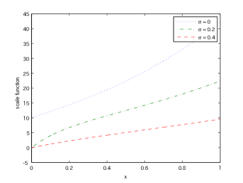
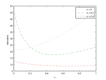
scale function $W^{(q)}$	derivative $W^{(q)^{\prime}}$

Figure 1. Scale functions and their derivatives for the case with Weibull-distributed jumps.

Figure 2. Value function $v_{\pi_{a^{*}}}$of the classical dividend problem.

We now consider the extensions described in the end of Section 2. Here we use the same parameters as in the results above. Figure 3 shows the results on the bail-out problem (Avram et al., , 2007) when $\varphi=1.3$. It plots $G$ in (2.18) as well as the value function $\overline{v}_{d^{*}}$ in (2.21). Here the optimal barrier level is obtained by computing the unique level $d^{*}$ that satisfies $G(d^{*})=0$. Figure 4 shows the results on the extension with terminal values at ruin (Loeffen and Renaud, , 2010) with the plots of $F$ in (2.22) and the value function $\widetilde{v}_{b^{*}}$ in (2.25). We consider the case with constant terminal value (i) $S=-1$ and $K=0$ and (ii) $S=1$ and $K=0$. The maximizer of $F$ becomes the barrier level $b^{*}$. Figure 5 shows the value functions $v_{c_{2}^{*}}$ on the extension with transaction costs (Loeffen, 2009b, ) when (i) $\delta=0.5$ and (ii) $\delta=0.1$. In order to obtain the optimal impulse contol $(c_{1}^{*},c_{2}^{*})$, we use the technique discussed in Section 4 of Loeffen, 2009b . Unlike the other results, the value functions are no longer monotone in $\sigma$ unless $\delta$ is sufficiently small. However, as $\delta$ decreases to zero, $c_{1}^{*}$ converges to $c_{2}^{*}$ and the value function converges to that of the classical model as shown in Figure 2.

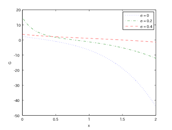
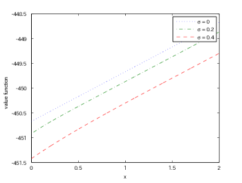
$G(x)$	value function $\overline{v}_{d^{*}}$

Figure 3. Bail-out problem: $G$ in (2.18) and the value function $\overline{v}_{d^{*}}$ when $\varphi=1.3$. Optimal barriers are $0.38$, $0.775$ and $1.495$ for $\sigma=0,0.2$ and $0.4$, respectively.

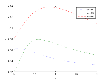
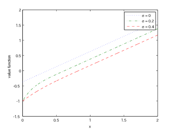
$F(x)$ when (i) $S=-1,K=0$	value function $\widetilde{v}_{b^{*}}$ when (i) $S=-1,K=0$
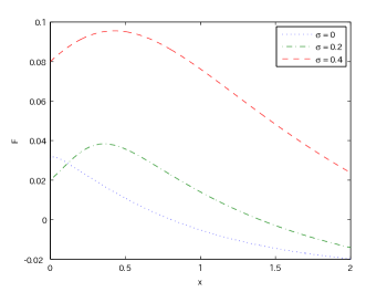
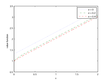
$F(x)$ when (ii) $S=1,K=0$	value function $\widetilde{v}_{b^{*}}$ when (ii) $S=1,K=0$

Figure 4. Extension with terminal values at ruin: $F$ in (2.22) and the value function $\widetilde{v}_{b^{*}}$ when (i) $S=-1,K=0$ and (ii) $S=1,K=0$. The optimal barriers are (i) $0.0628$, $0.0793$ and $0.1384$ and (ii) $0.0317$, $0.0383$ and $0.0955$, respectively, for $\sigma=0,0.2$ and $0.4$.

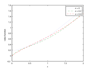
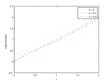
value function $v_{c_{2}^{*}}$ when (i) $\beta=0.5$	value function $v_{c_{2}^{*}}$ when (ii) $\beta=0.1$

Figure 5. Extension with transaction costs: value function when (i) $\beta=0.5$ and (ii) $\beta=0.1$. The optimal impulse controls $(c_{1}^{*},c_{2}^{*})$ are (i) $(0,1.173)$, $(0.069,1.527)$ and $(0,1.885)$ and (ii) $(0,0.05)$, $(0.222,0.481)$ and $(0.197,0.643)$ for $\sigma=0,0.2$ and $0.4$, respectively.

5.2. Numerical results on the $\beta$-class and CGMY process

We now consider, as an example of meromorphic Lévy processes, the $\beta$-class introduced by Kuznetsov, 2009a . The following definition is due to Kuznetsov, 2009a , Definition 4.

Definition 5.1.

A spectrally negative Lévy process is said to be in the $\beta$-class if its Lévy measure is in the form

(5.1) $$\nu({\rm d}x)=c\frac{e^{\alpha\beta x}}{(1-e^{\beta x})^{\lambda}}1_{\{x<0\}}{\rm d}x,\quad x\in\mathbb{R},$$

for some $\alpha>0$, $\beta>0$, $c\geq 0$ and $\lambda\in(0,3)$. It is equivalent to saying that its Laplace exponent is

$$\psi(z)=\hat{\mu}z+\frac{1}{2}\sigma^{2}z^{2}+\frac{c}{\beta}\left\{B(\alpha+\frac{z}{\beta},1-\lambda)-B(\alpha,1-\lambda)\right\}$$

where $B$ is the beta function $B(x,y):=\Gamma(x)\Gamma(y)/\Gamma(x+y)$.

The special case $\sigma=0$ and $\beta=1$ reduces to the class of Lamperti-stable processes, which are obtained by the Lamperti transformation (Lamperti, (1972)) from the stable processes conditioned to stay positive; see Bertoin and Yor, (2001) and Caballero et al., (2008) and references therein. For the scale function of a related process, see Kyprianou and Rivero, (2008).

It can be also seen that this is a “discrete-version” of the (spectrally negative) CGMY process, whose Lévy measure is given by

(5.2) $$\nu({\rm d}x)=c\frac{e^{\alpha x}}{|x|^{\lambda}}1_{\{x<0\}}{\rm d}x,\quad x\in\mathbb{R}.$$

Indeed, if we set $c=\widetilde{c}\beta^{\lambda}$ and $\alpha=\widetilde{\alpha}\beta^{-1}$ in (5.1), we have

(5.3) $$c\frac{e^{\alpha\beta x}}{(1-e^{\beta x})^{\lambda}}1_{\{x<0\}}\xrightarrow{\beta\downarrow 0}\widetilde{c}\frac{e^{\widetilde{\alpha}x}}{|x|^{\lambda}}1_{\{x<0\}},\quad x\in\mathbb{R}.$$

See Asmussen et al., (2007) for approximation of (double-sided) CGMY processes using hyperexponential distributions.

We shall use the results in Section 4 to obtain the bounds on the scale functions and the solutions to the classical optimal dividend problem. Figure 6 shows the approximation results when $q=0.03$, $\sigma=0.2$, $\hat{\mu}=0.1$, $\lambda=1.5$, $\alpha=3$, $\beta=1$ and $c=0.1$ in (5.1). We plot, for $m=15$ and $m=150$, the upper and lower bounds on the scale function, its derivative and the function $u_{a^{*}}$ defined in (2.16). As shown in the previous section, the difference between the upper and lower bounds indeed converges to zero.

We now take $\beta$ in (5.3) to zero and see how the approximation for the CGMY process works. Here we set $\tilde{\alpha}=3$ and $\tilde{c}=0.1$ and use the same values as the above for the other parameters. Figure 7 shows the upper and lower bounds of scale function and its derivative for various values of $\beta$. Figure 8 shows the mean value of the upper and lower bounds on the function $u$. Here we can indeed observe the convergence as $\beta\rightarrow 0$. This implies that it effectively approximates the scale function and the solution for the CGMY case.

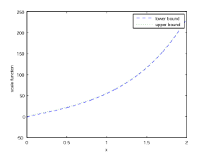
Bounds on $W^{(q)}(x)$ when $m=15$	Bounds on $W^{(q)}(x)$ when $m=150$
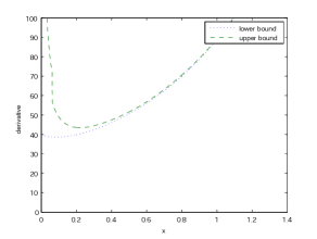
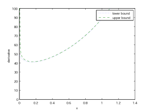
Bounds on $W^{(q)^{\prime}}(x)$ when $m=15$	Bounds on $W^{(q)^{\prime}}(x)$ when $m=150$
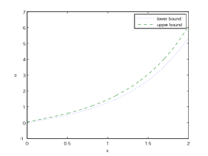
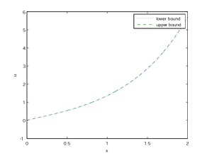
Bounds on $u(x)$ when $m=15$	Bounds on $u(x)$ when $m=150$

Figure 6. Approximation of the scale function and its derivative for the $\beta$-class.

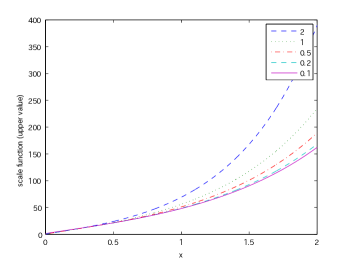
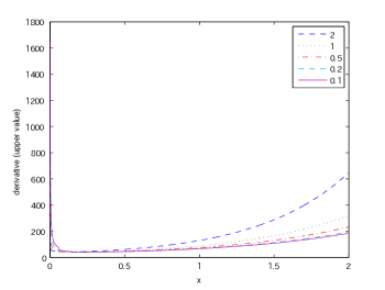
upper bounds for the scale functions	upper bounds for the derivatives
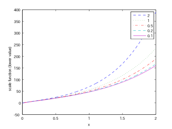
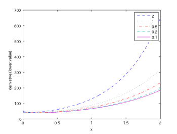
lower bounds for the scale functions	lower bounds for the derivatives

Figure 7. Convergence of scale functions to the CGMY model.

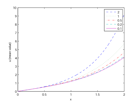
Figure 8. Convergence of $u$ to the CGMY model. Here we use $M=150$.

Appendix A Proofs

A.1. Proof of Lemmas 3.1 and 3.2

By (3.6), it is easy to verify that

$$\mathbb{E}^{x}\left[e^{-q\tau_{a}}1_{\{\tau_{a}<\infty\}}\right]=\sum_{i=1}^{n}\sum_{k=1}^{m_{i}}A_{i,q}^{(k)}\xi_{i,q}\int_{x-a}^{\infty}\frac{(\xi_{i,q}y)^{k-1}}{(k-1)!}e^{-\xi_{i,q}y}{\rm d}y,\quad 0\leq a<x,$$

and hence, because $W^{(q)}\in C^{1}(0,\infty)$,

(A.1) $$\frac{\partial}{\partial a}\mathbb{E}^{x}\left[e^{-q\tau_{a}}1_{\{\tau_{a}<\infty\}}\right] =\sum_{i=1}^{n}\sum_{k=1}^{m_{i}}A_{i,q}^{(k)}\xi_{i,q}\frac{(\xi_{i,q}(x-a))^{k-1}}{(k-1)!}e^{-\xi_{i,q}(x-a)},\quad 0\leq a<x,$$

(A.2) $$\left.\frac{\partial}{\partial x}\mathbb{E}^{x}\left[e^{-q\tau_{0}}1_{\{\tau_{0}<\infty\}}\right]\right|_{x=0+} =-\sum_{i=1}^{n}A_{i,q}^{(1)}\xi_{i,q}.$$

In fact, different representations of (A.1) and (A.2) can be pursued. By Theorem 8.1 of Kyprianou, (2006) and (2.9),

$$\mathbb{E}^{x}\left[e^{-q\tau_{a}}1_{\{\tau_{a}<\infty\}}\right]=Z^{(q)}(x-a)-\frac{q}{\zeta_{q}}W^{(q)}(x-a)=1+q\int_{0}^{x-a}W^{(q)}(y){\rm d}y-\frac{q}{\zeta_{q}}e^{\zeta_{q}(x-a)}W_{\zeta_{q}}(x-a)$$

for every $0\leq a<x$. Its derivative with respect to $a$ becomes

(A.3) $$\begin{split}\frac{\partial}{\partial a}\mathbb{E}^{x}\left[e^{-q\tau_{a}}1_{\{\tau_{a}<\infty\}}\right]&=-qW^{(q)}(x-a)+qe^{\zeta_{q}(x-a)}W_{\zeta_{q}}(x-a)+\frac{q}{\zeta_{q}}{e^{\zeta_{q}(x-a)}}W_{\zeta_{q}}^{\prime}(x-a)\\ &=\frac{q}{\zeta_{q}}{e^{\zeta_{q}(x-a)}}W_{\zeta_{q}}^{\prime}(x-a).\end{split}$$

In particular, when $a=0$, the derivative with respect to $x$ and its limit as $x\rightarrow 0$ are

(A.4) $$\frac{\partial}{\partial x}\mathbb{E}^{x}\left[e^{-q\tau_{0}}1_{\{\tau_{0}<\infty\}}\right]=-\frac{q}{\zeta_{q}}\left[-\zeta_{q}W^{(q)}(x)+W^{(q)^{\prime}}(x)\right]\xrightarrow{x\downarrow 0+}-\frac{q}{\zeta_{q}}\left[-\zeta_{q}W^{(q)}(0)+W^{(q)^{\prime}}(0+)\right]=-\frac{q}{\zeta_{q}}\theta.$$

By matching (A.2) and (A.4), Lemma 3.1 is immediate.

For the proof of Lemma 3.2, by matching (A.1) and (A.3) and using Lemma 3.1, we have

$$W_{\zeta_{q}}^{\prime}(y) =\frac{\theta}{\varrho_{q}}\sum_{i=1}^{n}\sum_{k=1}^{m_{i}}A_{i,q}^{(k)}\xi_{i,q}\frac{(\xi_{i,q}y)^{k-1}}{(k-1)!}e^{-(\zeta_{q}+\xi_{i,q})y}$$

$$=\frac{\theta}{\varrho_{q}}\sum_{i=1}^{n}\sum_{k=1}^{m_{i}}A_{i,q}^{(k)}(\zeta_{q}+\xi_{i,q})\left(\frac{\xi_{i,q}}{\zeta_{q}+\xi_{i,q}}\right)^{k}\frac{((\zeta_{q}+\xi_{i,q})y)^{k-1}}{(k-1)!}e^{-(\zeta_{q}+\xi_{i,q})y},\quad y\geq 0.$$

Integrating the above and changing variables, we have

$$W_{\zeta_{q}}(x)-W_{\zeta_{q}}(0)=\frac{\theta}{\varrho_{q}}\sum_{i=1}^{n}\sum_{k=1}^{m_{i}}A_{i,q}^{(k)}\left(\frac{\xi_{i,q}}{\zeta_{q}+\xi_{i,q}}\right)^{k}\frac{1}{(k-1)!}\int_{0}^{(\zeta_{q}+\xi_{i,q})x}{z^{k-1}}e^{-z}{\rm d}z,\quad x\geq 0.$$

Lemma 3.2 is now immediate because the integral part is a lower incomplete gamma function.

A.2. Proof of Proposition 4.2

Notice, for every $m\geq 1$, that

(A.5) $$\begin{split}&0\leq\sum_{k=1}^{m}\left(C_{k,q}-C_{k,q}^{(m)}\right)\leq\kappa_{q}-\sum_{k=1}^{m}C_{k,q}^{(m)}=\delta_{m},\\ &0\leq\sum_{k=m+1}^{\infty}C_{k,q}=\kappa_{q}-\sum_{k=1}^{m}C_{k,q}\leq\kappa_{q}-\sum_{k=1}^{m}C_{k,q}^{(m)}=\delta_{m},\end{split}$$

and hence by (A.5)

$$0\leq\overline{W}_{\zeta_{q}}^{(m)}(x)-W_{\zeta_{q}}(x)=\sum_{k=1}^{m}\left(C_{k,q}-C_{k,q}^{(m)}\right)e^{-(\zeta_{q}+\xi_{i,q})x}+\sum_{k=m+1}^{\infty}C_{k,q}e^{-(\zeta_{q}+\xi_{k,q})x}\\ \leq e^{-\zeta_{q}x}\sum_{k=1}^{m}\left(C_{k,q}-C_{k,q}^{(m)}\right)+e^{-(\zeta_{q}+\xi_{{m+1},q})x}\sum_{k=m+1}^{\infty}C_{k,q}\leq\delta_{m}\left[e^{-\zeta_{q}x}+e^{-(\zeta_{q}+\xi_{m+1,q})x}\right].$$

Therefore we have the bounds for $W_{\zeta_{q}}$ in (4.10). The bounds for $W^{(q)}$ are immediate by multiplying $e^{\zeta_{q}x}$. Finally, the convergence results hold because $\delta_{m}\rightarrow 0$ and $e^{-\zeta_{q}x}+e^{-(\zeta_{q}+\xi_{m+1,q})x}$ and $1+e^{-\xi_{m+1,q}x}$ are bounded uniformly in $x\geq 0$.

A.3. Proof of Proposition 4.3

The lower bound is immediate by the fact that $0\leq C_{i,q}^{(m)}\leq C_{i,q}$. For every $x\geq 0$, we have by (A.5)

$$W^{(q)^{\prime}}(x) =(\psi^{\prime}(\zeta_{q}))^{-1}\zeta_{q}e^{\zeta_{q}x}+\sum_{i=1}^{\infty}C_{i,q}\xi_{i,q}e^{-\xi_{i,q}x}$$

$$=\underline{w}^{(m)}(x)+\sum_{i=1}^{m}(C_{i,q}-C_{i,q}^{(m)})\xi_{i,q}e^{-\xi_{i,q}x}+\sum_{i=m+1}^{\infty}C_{i,q}\xi_{i,q}e^{-\xi_{i,q}x}$$

$$\leq\underline{w}^{(m)}(x)+\max_{1\leq k\leq m}(\xi_{k,q}e^{-\xi_{k,q}x})\sum_{i=1}^{m}(C_{i,q}-C_{i,q}^{(m)})+\max_{k\geq m+1}(\xi_{k,q}e^{-\xi_{k,q}x})\sum_{i=m+1}^{\infty}C_{i,q}$$

$$\leq\underline{w}^{(m)}(x)+\left[\max_{1\leq k\leq m}(\xi_{k,q}e^{-\xi_{k,q}x})+\max_{k\geq m+1}(\xi_{k,q}e^{-\xi_{k,q}x})\right]\delta_{m}=\overline{w}^{(m)}(x),$$

which shows the first claim. For the second claim, notice that for the given $x_{0}>0$,

$$0\leq\overline{w}^{(m)}(x)-\underline{w}^{(m)}(x)\leq\left[\max_{1\leq k\leq m}(\xi_{k,q}e^{-\xi_{k,q}x_{0}})+\max_{k\geq m+1}(\xi_{k,q}e^{-\xi_{k,q}x_{0}})\right]\delta_{m}$$

uniformly on $[x_{0},\infty)$. Because $\delta_{m}$ vanishes as $m\rightarrow 0$ and $\sup_{\lambda\geq 0}\lambda e^{-\lambda x}<\infty$, the convergence is immediate.

A.4. Proof of Corollary 4.2

We have

$$W^{(q)^{\prime}}(x) =\underline{w}^{(m)}(x)+\sum_{i=1}^{m}(C_{i,q}-C_{i,q}^{(m)})\xi_{i,q}e^{-\xi_{i,q}x}+\sum_{i=m+1}^{\infty}C_{i,q}\xi_{i,q}e^{-\xi_{i,q}x}$$

$$\leq\underline{w}^{(m)}(x)+\max_{1\leq k\leq m}(\xi_{k,q}e^{-\xi_{k,q}x})\sum_{i=1}^{m}(C_{i,q}-C_{i,q}^{(m)})+\frac{\zeta_{q}}{q}e^{-\xi_{m+1,q}x}\sum_{i=m+1}^{\infty}A_{i,q}\xi_{i,q}$$

$$\leq\underline{w}^{(m)}(x)+\max_{1\leq k\leq m}(\xi_{k,q}e^{-\xi_{k,q}x})\delta_{m}+\epsilon_{m}e^{-\xi_{m+1,q}x}$$

where the last inequality holds because

$$\frac{\zeta_{q}}{q}\sum_{k=m+1}^{\infty}\xi_{i,q}A_{i,q}=\theta-\frac{\zeta_{q}}{q}\sum_{k=1}^{m}\xi_{i,q}A_{i,q}\leq\theta-\frac{\zeta_{q}}{q}\sum_{k=1}^{m}\xi_{i,q}A_{i,q}^{(m)}=\epsilon_{m},\quad m\geq 1.$$

This together with Proposition 4.3 shows the claim.

References

- Alili and Kyprianou, (2005) Alili, L. and Kyprianou, A. E. (2005). Some remarks on first passage of Lévy processes, the American put and pasting principles. Ann. Appl. Probab., 15(3):2062–2080.
- Asmussen, (1996) Asmussen, S. (1996). Fitting phase-type distributions via the em algorithm. Scand. J. Statist, 23:419–441.
- Asmussen et al., (2004) Asmussen, S., Avram, F., and Pistorius, M. R. (2004). Russian and American put options under exponential phase-type Lévy models. Stochastic Process. Appl., 109(1):79–111.
- Asmussen et al., (2007) Asmussen, S., Madan, D., and Pistorius, M. (2007). Pricing equity default swaps under an approximation to the CGMY levy model. Journal of Computational Finance, 11(2):79–93.
- Asmussen and Taksar, (1997) Asmussen, S. and Taksar, M. (1997). Controlled diffusion models for optimal dividend pay-out. Insurance: Math. Econom., 20:1–15.
- Avram et al., (2004) Avram, F., Kyprianou, A. E., and Pistorius, M. R. (2004). Exit problems for spectrally negative Lévy processes and applications to (Canadized) Russian options. Ann. Appl. Probab., 14(1):215–238.
- Avram et al., (2007) Avram, F., Palmowski, Z., and Pistorius, M. R. (2007). On the optimal dividend problem for a spectrally negative Lévy process. Ann. Appl. Probab., 17(1):156–180.
- Azcue and Muler, (2005) Azcue, P. and Muler, N. (2005). Optimal reinsurance and dividend distribution policies in the Cramér-Lundberg model. Math. Finance, 15(2):261–308.
- Barndorff-Nielsen, (1998) Barndorff-Nielsen, O. E. (1998). Processes of normal inverse Gaussian type. Finance Stoch., 2(1):41–68.
- Baurdoux and Kyprianou, (2008) Baurdoux, E. and Kyprianou, A. E. (2008). The McKean stochastic game driven by a spectrally negative Lévy process. Electron. J. Probab., 13:no. 8, 173–197.
- Baurdoux and Kyprianou, (2009) Baurdoux, E. and Kyprianou, A. E. (2009). The shepp-shiryaev stochastic game driven by a spectrally negative lévy process. Theory of Probability and Its Applications, 53.
- Bertoin, (1996) Bertoin, J. (1996). Lévy processes, volume 121 of Cambridge Tracts in Mathematics. Cambridge University Press, Cambridge.
- Bertoin and Yor, (2001) Bertoin, J. and Yor, M. (2001). On subordinators, self-similar Markov processes and some factorizations of the exponential variable. Electron. Comm. Probab., 6:95–106 (electronic).
- Bladt et al., (2003) Bladt, M., Gonzalez, A., and Lauritzen, S. L. (2003). The estimation of phase-type related functionals using Markov chain Monte Carlo methods. Scand. Actuar. J., (4):280–300.
- Caballero et al., (2008) Caballero, M., Pardo, J., and Pérez, J. (2008). On lamperti stable processes. Preprint.
- Caballero and Chaumont, (2006) Caballero, M. E. and Chaumont, L. (2006). Conditioned stable Lévy processes and the Lamperti representation. J. Appl. Probab., 43(4):967–983.
- Carr et al., (2002) Carr, P., Hélyette, G., Madan, D. B., and Yor, M. (2002). The structure of asset returns: an emperical investigation. Journal of Business, 75:305–332.
- Chan et al., (2009) Chan, T., Kyprianou, A., and Savov, M. (2009). Smoothness of scale functions for spectrally negative Lévy processes. Probability Theory and Related Fields.
- Chaumont et al., (2009) Chaumont, L., Kyprianou, A. E., and Pardo, J. C. (2009). Some explicit identities associated with positive self-similar Markov processes. Stochastic Process. Appl., 119(3):980–1000.
- De Finetti, (1957) De Finetti, B. (1957). Su un’impostazion alternativa dell teoria collecttiva del rischio. Trans. XVth Internat. Congr. Actuaries, 2:433–443.
- Eberlein et al., (1998) Eberlein, E., Keller, U., and Prause, K. (1998). New insights into smile, mispricing and value at risk: the hyperbolic model. Journal of Business, 71:371–405.