Entropy Production in Gluodynamics
in temporal axial gauge in 2+1 dimensions

Abstract

Entropy production in non-Abelian gauge theory is discussed in the limit of vanishing classical fields. Based on the Kadanoff-Baym equation with the leading order self-energy in the temporal axial gauge, the kinetic entropy is introduced and is proven to increase for a given self-energy. Numerical simulation of the Kadanoff-Baym equation for the non-Abelian gauge theory is performed in 2+1 dimensions. Starting from anisotropic distribution in momentum space, relaxation to isotropic distribution proceeds and the entropy is produced due to off-shell scattering of massive transverse polarization mode as expected from the proof of the H-theorem.

1 Introduction

In heavy-ion collisions at the Relativistic Heavy Ion Collider (RHIC), it is plausible from theoretical arguments and experimental evidences that a new form of matter made of quarks and gluons is created.[1] This matter referred to as a strongly coupled QGP (sQGP)[2] is characterized by its strongly interacting nature; the shear viscosity is extremely small and the thermalization time is very short. Hydrodynamic models successfully describe the radial and elliptic flows at RHIC,[3, 4] and they require a local thermal equilibrium in the early stage. Comparison with the experimental results of the elliptic flow suggests that a thermalization time of the partons is about 0.6-1 fm$/c$.[3] This short thermalization time seems to contradict the perturbative estimate,[5] and it is compatible with the formation time of partons. This means that the Boltzmann equation would have serious problems in describing the thermalization of dense systems, such as glasma, formed in the early stage of collisions.

At lower energies, hadronic transport models based on the Boltzmann equation have been successfully applied to heavy-ion collisions including nuclear fragment formation,[6] flavor production,[7] particle spectra,[8] and collective flows.[9] By comparison, hadronic transport models fail to describe early thermalization and predict smaller elliptic flows at RHIC.[10] These successes and failures imply the formation of QGP at RHIC, and may also suggest the limitation of the Boltzmann equation in dense systems. Boltzmann approaches are based on the assumption that the particle interaction is rare and three particle collisions can be ignored, and the spectral function is narrow enough for the quasi-particle approximation to be valid. In dense matter formed at RHIC, one or both of these conditions are not satisfied. One of the prescriptions to implement multi-particle interaction is to apply the classical field theories.[11, 12, 13, 14, 15] When the gluon density is so high that gluons are combined to form finite color glass condensate, a large part of the energy density is stored in the classical field. It is generally believed that the early thermalization is realized from rapid growth of intense classical Yang-Mills fields triggered by the plasma instabilities.[11, 12, 13, 14, 16, 17] The decay of strong gluon field into quarks and gluons needs quantum field description in nonequilibrium conditions. In addition, classical field dynamics should not be applied to high momentum modes even in the dense early stage. Another aspect of dense systems, the spectral function change, can be described perturbatively or by using some kind of resummation in quantum field theories. Among various ways of resummation, the $\Phi$-derivable approach would be the most favorable, since it does not have the secularity problem, and leads to a correct equilibrium. Hence we should study the gluon thermalization processes based on nonequilibrium quantum field theories such as the Kadanoff-Baym equation based on $\Phi$-derivable approximation.

The Kadanoff-Baym (KB) equation, equivalently the Schwinger-Dyson equation, is given by Kadanoff and Baym [20, 21] in the reformulation of a functional technique with Green’s functions by Luttinger and Ward [22]. It is related to variational technique of an effective action using the so-called $\Phi$-derivable approximation, and is shown to satisfy the conservation laws of a system.[23] In the $\Phi$-derivable approximation, diagrams contributing to the self-energy are truncated with some expansion parameter. This technique is applied to relativistic systems and reformulated for nonequilibrium many body systems by using the Schwinger-Keldysh path integral formalism and 2-particle irreducible (2PI) effective action technique.[24, 25, 26, 27, 28]

Nonequilibrium quantum field theoretical approach is a tool to understand a large variety of contemporary problems in high energy particle physics, nuclear physics, astrophysics, cosmology, as well as condensed matter physics.[18, 19] In cosmology it is applied to describe the reheating process due to the decay of inflaton field coupled to the Higgs at the end stage of inflation.[29, 30, 31, 32] In condensed matter physics it is applied to Bose-Einstein Condensate. In this approach both conservation law and gapless Nambu-Goldstone excitation [33] are respected.[18, 34] It might be also possible to apply it to heavy ion collisions to describe equilibration processes of partons.[35]

With respect to numerical simulation, Danielewicz first carried out a pioneering work in 1984 [36] to describe heavy ion collisions with spectral functions at the non-relativistic energies. In the relativistic level, the equilibration processes are simulated in $\phi^{4}$ model in the symmetric phase in 1+1,[37, 38] 2+1 [39] and 3+1 [40, 41] dimensions. Numerical analyses have been also done in the broken phase in 1+1 [42] and 3+1 [40] dimensions. Recently simulations have been extended to the system in an expanding background.[31] Similarly based on the next-to-leading order self-energy in the systematic $1/N$ expansion,[43] simulations have been done both in the symmetric [44] and broken [32] phases in the $O(N)$ model. All of these analyses show that the thermalization proceeds; distribution functions lose information on the initial condition and converge to the Bose-Einstein distribution. Until now the KB equation for the non-Abelian gauge theories has never been solved numerically. This is because we have several problems such as gauge covariance of the equation of motion,[45, 46] infrared singularity, and violation of Ward identity.[47]

In this paper we discuss the gluon thermalization in the temporal axial gauge (TAG) on the basis of the KB equation with the 2PI effective action in the leading order of the coupling expansion. We expect that the off-shell particle number changing processes such as $g\leftrightarrow gg$ contribute to the entropy production in heavy ion collisions. These off-shell effects come from the gluon decay due to finite spectral width and memory integral in the KB equation. A part of $gg\leftrightarrow gg$ processes, $gg\leftrightarrow g\leftrightarrow gg$, is included in the present treatment via the sequential off-shell processes of $gg\leftrightarrow g$ and $g\leftrightarrow gg$, and contributes to thermalization. In the Boltzmann equation, $g\leftrightarrow gg$ is prohibited,[48] and the on-shell $gg\leftrightarrow ggg$ process is the most efficient in entropy production. It is known that the on-shell dynamics predicts a long equilibration time $\tau_{\rm eq}=2-3\mathrm{fm}/c$ [5], and it can not explain the early thermalization of glasma. Hence we investigate off-shell dynamics by using KB equation and give whether thermalization occurs or not due to the effects which have been neglected. The present entropy production mechanism from the off-shell gluons is different from the classical plasma instabilities, such as the Weibel [16, 12, 13, 14] and Nielsen-Olsen [17] types. Our approach is also different from classical statistical approach on a lattice, which conjectures the significance of the leading order and next-to-leading order resummed loop self-energy.[49] The aim in this paper is to show that the off-shell processes $g\to gg$ can contribute to equilibration of gluons. For this purpose, we introduce the concept of kinetic entropy and the H-theorem, and perform numerical simulations of the KB equation in gluodynamics. In order to avoid the problems mentioned above, we make some prescriptions and approximations, such as gauge fixing, infrared cutoff and simulation of only the transverse scattering contributions.

This paper is organized as follows. In Sec. 2, we write down the KB equation in gluodynamics for both transverse and longitudinal part of Green’s functions. As the self-energy, we take account of the leading order (LO) terms in the coupling expansion, which contain the off-shell $g\leftrightarrow gg$ processes. In Sec. 3, we introduce kinetic entropy, and by use of the gradient expansion as in Refs. IKV4,Kita,Nishiyama,Nishiyama:2010wc we show an analytical proof of the H-theorem for the given self-energy in order to examine whether the above leading order off-shell processes ($g\leftrightarrow gg$) can contribute to equilibration or not. The concept of entropy should also be extended to the systems with strong classical fields,[15] which is out of the scope in this paper. In Sec. 4, we give numerical results of the Kadanoff-Baym equations for the transverse scattering processes with massive mode in a spatially uniform $2+1$ dimensional spacetime in order to extract the effects of the off-shell particle number changing processes. We find that the off-shell particle number changing processes can actually contribute to entropy production and thermalization. We summarize our work in Sec. 5.

2 Kadanoff-Baym equation for gluons in Temporal Axial Gauge

In this section we write down the Kadanoff-Baym equation for gluons in the temporal axial gauge (TAG), $A_{0}=0$. This section focuses on the practical use of the KB equation. Let us neglect the classical field $\langle A\rangle=0$ and concentrate on the quantum fluctuations. We start with the Lagrangian density

$${\cal L}=-\frac{1}{4}F^{a\mu\nu}F^{a}_{\mu\nu}\ ,\quad A_{0}^{a}=0\ ,$$ (1)

where $F_{\mu\nu}=\partial_{\mu}A^{a}_{\nu}-\partial_{\nu}A^{a}_{\mu}+gf^{abc}A^{b}_{\mu}A^{c}_{\nu}$ and $f^{abc}$ is a structure constant in non-Abelian gauge theory. The Greek indices run over the coordinate space $\{0,1,\cdots,d\}$, and the color indices $\{a,b,\cdots\}$ run over $\{1,\cdots,N^{2}-1\}$. We use a closed time path $\cal C$ along the real time axis, the path from $t_{0}$ to $\infty$ and from $\infty$ to $t_{0}$ as shown in Fig. 1, in order to trace nonequilibrium dynamics.[24, 25] Then the 2PI effective action with vanishing classical field $(\langle A\rangle=0)$ is written as

$$\Gamma[D]=\frac{i}{2}{\rm Tr}{\ln}(D)^{-1}+\frac{i}{2}D_{0}^{-1}D+\frac{1}{2}\Gamma_{2}[D].$$ (2)

Here $iD_{0\ ij}^{-1}=-(\delta_{ij}\partial_{x}^{2}+\partial_{x,i}\partial_{x,j})\delta^{ab}\delta_{\cal C}(x-y)$ is the free Green’s function, and $D$ $(D^{00}=D^{0i}=D^{i0}=0$; $i,j,\cdots=1,\cdots,d)$ is the full Green’s function, both of which are defined on the closed time path ${\cal C}$. The remaining functional $\frac{1}{2}\Gamma_{2}[D]$ in (2) is a sum of the all possible 2PI graphs written with respect to $D$ which remains connected upon cutting two Green’s function lines. The stationary relation for the effective action (2), $\delta\Gamma/\delta D=0$, gives the Schwinger-Dyson equation for the Green’s function $D(x,y)$

$$D^{-1}(x,y)=D_{0}^{-1}(x,y)-\Pi(x,y)$$ (3)

or equivalently,

$$(\delta_{ik}\partial_{x}^{2}+\partial_{x,i}\partial_{x,k})D^{ab}_{kj}(x,y)+i\int_{\cal C}dz\Pi^{ac}_{ik}(x,z)D^{cb}_{kj}(z,y)=-i\delta^{ab}\delta_{ij}\delta_{\cal C}(x-y)$$ (4)

with the proper self-energy defined as $\Pi=i\delta\Gamma_{2}[D]/\delta D$. The self-energy is expressed as

$$\Pi(x,y)=-i\delta_{\cal C}(x-y)\Pi_{\rm loc}(x)+\Pi_{\rm nonl}(x,y)$$ (5)

where the local part $\Pi_{\rm loc}$ contributes to the mass shift while the non-local part $\Pi_{\rm nonl}$ induces the mode-coupling between the different wavenumbers.

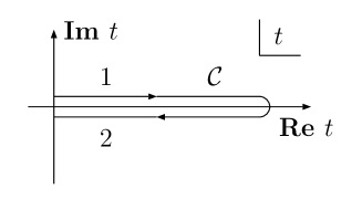
Figure 1: Integral path in the time coordinate.

We are now interested in $\{ij\}$ components of the Green’s function and the self-energy,[47] and shall decompose the two-point function $D_{ij}^{ab}(x,y)$ and the non-local part of the self-energy $\Pi_{{\rm nonl},ij}^{ab}$ into the statistical and spectral parts,

$$F_{ij}^{ab}=\frac{1}{2}\left[D^{21,ab}_{ij}+D^{12,ab}_{ij}\right]\ , \quad\rho_{ij}^{ab}=i\left[D^{21,ab}_{ij}-D^{12,ab}_{ij}\right]\ ,$$ (6)

$$\Pi_{F,ij}^{ab}(x,y)=\frac{1}{2}\left[\Pi_{{\rm nonl},ij}^{21,ab}+\Pi_{{\rm nonl},ij}^{12,ab}\right]\ , \quad\Pi_{\rho,ij}^{ab}(x,y)=i\left[\Pi_{{\rm nonl},ij}^{21,ab}-\Pi_{{\rm nonl},ij}^{12,ab}\right]\ .$$ (7)

The upper label ”1” represents the path from $t_{0}$ to $\infty$ and ”2” represents that from $\infty$ to $t_{0}$ in the closed time path contour $\cal C$. The spectral function $\rho(x,y)$ contains the information on which states are the most realized, while the statistical function $F(x,y)$ determines how much a state is occupied. The Schwinger-Dyson equation (3) can be equivalently rewritten in terms of $F_{ij}^{ab}(x,y)$ and $\rho_{ij}^{ab}(x,y)$ as coupled integro-differential equations

$$\left[(\delta_{ij}\partial_{x}^{2}+\partial_{x,i}\partial_{x,j})\delta^{ab}+\Pi_{{\rm loc},ij}^{ab}(x)\right]F_{jk}^{bc}(x,y) = \int_{t_{0}}^{y^{0}}dz\Pi_{F,ij}^{ab}(x,z)\rho^{bc}_{jk}(z,y)$$ (8)

$$- \int_{t_{0}}^{x^{0}}dz\Pi_{\rho,ij}^{ab}(x,z)F_{jk}^{bc}(z,y),$$

$$\left[(\delta_{ij}\partial_{x}^{2}+\partial_{x,i}\partial_{x,j})\delta^{ab}+\Pi_{{\rm loc},ij}^{ab}(x)\right]\rho_{jk}^{bc}(x,y) = -\int_{y^{0}}^{x^{0}}dz\Pi_{\rho,ij}^{ab}(x,z)\rho_{jk}^{bc}(z,y)$$ (9)

where $t_{0}$ is the initial time. The set of equations (8) and (9) is the Kadanoff-Baym equation of the gauge theory, which describes the time evolution of the fluctuations with $F$ and $\rho$. At each time step the spectral function $\rho_{ij}^{ab}(x,y)$ must satisfy the conditions following from the commutation relations:

$$\rho_{ij}^{ab}(x,y)|_{x^{0}\rightarrow y^{0}} = 0,$$

$$\partial_{x^{0}}\rho_{ij}^{ab}(x,y)|_{x^{0}\rightarrow y^{0}} = \delta_{ij}\delta^{ab}\delta^{d}({\bf x-y}),$$

$$\partial_{x^{0}}\partial_{y^{0}}\rho^{ab}_{ij}(x,y)|_{x^{0}\rightarrow y^{0}} = 0.$$ (10)

In this paper we restrict ourselves to the spatially homogeneous and color isotropic situation. From the translational invariance, we make a Fourier transformation of the Green’s functions and the self-energies with respect to the spatial relative coordinates, and decompose into the transverse and longitudinal components as

$$I^{ab}_{ij}(x^{0},y^{0};{\bf k}) = \delta^{ab}\left[\left(\delta_{ij}-\frac{k_{i}k_{j}}{{\bf k}^{2}}\right)I_{T}(x^{0},y^{0};{\bf k})+\frac{k_{i}k_{j}}{{\bf k}^{2}}I_{L}(x^{0},y^{0};{\bf k})\right],$$ (11)

where $I=D,\Pi,F,\rho,\Pi_{F},\Pi_{\rho}$ or $\Pi_{\rm loc}$. Then the KB equations of the transverse and longitudinal parts are simplified in the momentum space as

$$\left[\partial_{x,0}^{2}+{\bf k}^{2}+\Pi_{{\rm loc},T}(x^{0})\right]F_{T}(x^{0},y^{0};{\bf k})= \left\{\left[\Pi_{F,T}\rho_{T}\right]_{t_{0}}^{y^{0}}-\left[\Pi_{\rho,T}F_{T}\right]_{t_{0}}^{x^{0}}\right\}\ ,$$ (12a)

$$\left[\partial_{x,0}^{2}+{\bf k}^{2}+\Pi_{{\rm loc},T}(x^{0})\right]\rho_{T}(x^{0},y^{0};{\bf k})= -\left[\Pi_{\rho,T}\rho_{T}\right]_{y^{0}}^{x^{0}}\ ,$$ (12b)

$$\left[\partial_{x,0}^{2}+\Pi_{{\rm loc},L}(x^{0})\right]F_{L}(x^{0},y^{0},{\bf k})= \left\{\left[\Pi_{F,L}\rho_{L}\right]_{t_{0}}^{y^{0}}-\left[\Pi_{\rho,L}F_{L}\right]_{t_{0}}^{x^{0}}\right\}\ ,$$ (13a)

$$\left[\partial_{x,0}^{2}+\Pi_{{\rm loc},L}(x^{0})\right]\rho_{L}(x^{0},y^{0};{\bf k})= -\left[\Pi_{\rho,L}\rho_{L}\right]_{y^{0}}^{x^{0}}\ ,$$ (13b)

where we have introduced a short-hand notation,

$$\left[AB\right]_{t_{1}}^{t_{2}}\equiv\int_{t_{1}}^{t_{2}}dz^{0}A(x^{0},z^{0};{\bf k})B(z^{0},y^{0};{\bf k})\ .$$ (14)

Figure 2: Leading order self energy for gluons.

We approximate the self-energy $\Pi$ with the skeleton diagrams obtained at the leading order in $g^{2}$ which is depicted in Fig.2. The transverse and longitudinal parts are explicitly given in terms of $D_{T}$ and $D_{L}$ as

$$\Pi_{{\rm loc},T}(x^{0}) = g^{2}N\int\frac{d^{d}p}{(2\pi)^{d}}\left[(d-2)D_{T}+D_{L}+\frac{\sin^{2}\theta_{{\bf p},{\bf k}}}{d-1}(D_{T}-D_{L})\right]\ ,$$ (15)

$$\Pi_{{\rm loc},L}(x^{0}) = g^{2}N\int\frac{d^{d}p}{(2\pi)^{d}}\left[(d-1)D_{T}+(D_{L}-D_{T})\sin^{2}\theta_{{\bf p},{\bf k}}\right]\ ,$$ (16)

where the arguments of $D$ in the integral is $(x^{0},x^{0};{\bf p})$. Similarly the transverse and longitudinal components of the nonlocal part $\Pi_{\rm nonl}$ are given as

$$\Pi_{{\rm nonl},T}(x^{0},y^{0};-{\bf k})= -\frac{g^{2}N}{2(d-1)}\int\frac{d^{d}p}{(2\pi)^{d}}\sum_{\alpha,\beta}P_{\alpha\beta}({\bf p},-{\bf p}-{\bf k})D_{\alpha}({\bf p})D_{\beta}({\bf-p-k})\ ,$$ (17)

$$\Pi_{{\rm nonl},L}(x^{0},y^{0};-{\bf k})= -\frac{g^{2}N}{2}\int\frac{d^{d}p}{(2\pi)^{d}}\sum_{\alpha,\beta}Q_{\alpha\beta}({\bf p},-{\bf p}-{\bf k})D_{\alpha}({\bf p})D_{\beta}({\bf-p-k})\ ,$$ (18)

where the sum runs over $\alpha\beta=TT,LT,TL$ and $LL$. In the integral, the temporal variables for $D_{\alpha}$ and $D_{\beta}$ are $(x^{0},y^{0})$. Here $P_{\alpha\beta}$ and $Q_{\alpha\beta}$ are given as follows

$$P_{TT}({\bf p},{\bf q})= P_{TT}^{(1)}({\bf p},{\bf q})+P_{TT}^{(1)}({\bf q},-{\bf p}-{\bf q})+P_{TT}^{(1)}(-{\bf p}-{\bf q},{\bf p})\ ,$$ (19a)

$$Q_{TT}({\bf p},{\bf q})= \frac{[({\bf p}+{\bf q})\cdot({\bf p}-{\bf q})]^{2}}{({\bf p}+{\bf q})^{2}}\,\left[d-2+\frac{({\bf p}\cdot{\bf q})^{2}}{{\bf p}^{2}{\bf q}^{2}}\right]\ ,$$ (19b)

$$P_{LL}({\bf p},{\bf q})= ({\bf p}+{\bf q})^{2}\left[1-\frac{({\bf p}\cdot{\bf q})^{2}}{{\bf p}^{2}{\bf q}^{2}}\right]\ ,$$ (19c)

$$P_{LT}({\bf p},{\bf q})= P_{TL}({\bf q},{\bf p})=Q_{TT}({\bf q},-{\bf p}-{\bf q})\ ,$$ (19d)

$$Q_{LT}({\bf p},{\bf q})= Q_{TL}({\bf q},{\bf p})=P_{LL}({\bf p},-{\bf p}-{\bf q})\ ,$$ (19e)

$$Q_{LL}({\bf p},{\bf q})= 0\ ,$$ (19f)

where $P_{TT}^{(1)}$ is given as

$$P_{TT}^{(1)}({\bf p},{\bf q})= 4(d-1)\left[{\bf p}^{2}-\frac{({\bf p}\cdot({\bf p}+{\bf q}))^{2}}{({\bf p}+{\bf q})^{2}}\right]$$

$$- \frac{4}{3}({\bf p}+{\bf q})^{2}\left[1-\frac{({\bf p}\cdot({\bf p}+{\bf q}))^{2}}{{\bf p}^{2}({\bf p}+{\bf q})^{2}}\right]\left[1-\frac{({\bf q}\cdot({\bf p}+{\bf q}))^{2}}{{\bf q}^{2}({\bf p}+{\bf q})^{2}}\right]\ .$$ (20)

We find several characteristic features of these coefficients. First, $P_{\alpha\beta}$ and $Q_{\alpha\beta}$ are all semi-positive definite for $d\geq 2$,

$$P_{\alpha\beta}\geq 0\ ,\quad Q_{\alpha\beta}\geq 0\quad(d\geq 2)\ .$$ (21)

Next, we find some symmetric relations. For example, $P_{TT}$ is symmetric for any exchange of the variables ${\bf p},{\bf q}$ and ${\bf k}$, which satisfy ${\bf p}+{\bf q}+{\bf k}={\bf 0}$,

$$P_{TT}({\bf p},{\bf q})=P_{TT}({\bf q},{\bf k})=P_{TT}({\bf k},{\bf p})=P_{TT}({\bf q},{\bf p})\ .$$ (22)

By using the identity,

$${\bf p}^{2}-\frac{[{\bf p}\cdot({\bf p}+{\bf q})]^{2}}{({\bf p}+{\bf q})^{2}}= {\bf q}^{2}-\frac{[{\bf q}\cdot({\bf p}+{\bf q})]^{2}}{({\bf p}+{\bf q})^{2}}\ ,$$ (23)

we find that $P_{TT}^{(1)}$ is symmetric under the exchange of ${\bf p}$ and ${\bf q}$, and the cyclic sum of $P_{TT}^{(1)}$ leads to the cyclic symmetry. Other symmetric coefficients ($Q_{TT}$ and $P_{LL}$) are also symmetric under the exchange of two momentum,

$$Q_{TT}({\bf p},{\bf q})=Q_{TT}({\bf q},{\bf p})\ ,\quad P_{LL}({\bf p},{\bf q})=P_{LL}({\bf q},{\bf p})\ .$$ (24)

For mixed coefficients ($P_{LT},P_{TL},Q_{LT},Q_{TL}$) Eqs. (19d) and (19e) are rewritten by using these vectors (${\bf p},{\bf q},{\bf k}$) as,

$$P_{LT}({\bf k},{\bf p})=P_{TL}({\bf p},{\bf k})=Q_{TT}({\bf p},{\bf q})\ ,\quad Q_{LT}({\bf p},{\bf q})=Q_{TL}({\bf q},{\bf p})=P_{LL}({\bf p},{\bf k})\ .$$ (25)

These relations are useful to prove the H-theorem as discussed later.

In the limit of ${\bf k}\rightarrow 0$, we can reproduce the mass shift derived by using the Schwinger-Dyson equation in thermal equilibrium,[47]

$$\Pi_{ii}(x^{0},y^{0})= g^{2}N(d-1)\int\frac{d^{d}p}{(2\pi)^{d}}\Big{[}-i\delta(x^{0}-y^{0})[(d-1)D_{T}(x^{0},y^{0};{\bf p})+D_{L}(x^{0},y^{0};{\bf p})]$$

$$-{\bf p}^{2}D_{T}(x^{0},y^{0};{\bf p})\left[2D_{T}(x^{0},y^{0};{\bf p})+D_{L}(x^{0},y^{0};{\bf p})\right]\Big{]}\ ,$$ (26)

where $\Pi_{ii}=(d-1)\Pi_{T}+\Pi_{L}$. This result is consistent with the hard thermal loop (HTL) approximation.[47, 54] As already discussed in Ref. KajantieKapusta1985, the Ward-Takahashi identity is not satisfied in the KB equation with 2PI effective action, because diagrams with different orders in $g^{2}$ are resummed.

3 Proof of the H-theorem for the non-Abelian gauge theory

In this section we give the expression of the kinetic entropy in terms of the two-point Green’s functions $D(x,y)$ for the non-Abelian gauge theory. We shall investigate the case with vanishing classical fields $\langle A\rangle=0$ and color isotropic Green’s functions $D^{ab}(x,y)=\delta^{ab}D(x,y)$ in the temporal axial gauge $A^{a}_{0}=0$. Then we find that the kinetic entropy satisfies the H-theorem. To be generic, we here consider non-uniform system. In the leading order of the gradient expansion, we can still utilize the same coefficients $P_{\alpha\beta}$ and $Q_{\alpha\beta}$ as those shown for the uniform system in the previous section, since the modification of these coefficients are in the higher order in the gradient expansion as discussed later.

The KB equations for the transverse and longitudinal components, Eqs. (12a)-(13b), have a similar form to that for the scalar field theory, then the kinetic entropy current would have a similar form to that derived in the scalar theory.[50, 51, 52, 53, 55, 56, 57, 58, 59] We start from a conjecture that the kinetic entropy current per color in the gauge theory with temporal axial gauge is given by

$${s}^{\mu}\equiv \int\!\frac{d^{d+1}k}{(2\pi)^{d+1}}(d-1)\left[\left(k^{\mu}-\frac{1}{2}\frac{\partial{\rm Re}\ \Pi_{T,{\rm R}}}{\partial k_{\mu}}\right)\frac{\rho_{T}}{i}+\frac{1}{2}\frac{\partial{\rm Re}\ D_{T,{\rm R}}}{\partial k_{\mu}}\frac{\Pi_{\rho,T}}{i}\right]\sigma(f_{T})$$

$$+ \int\!\frac{d^{d+1}k}{(2\pi)^{d+1}}\left[\left(k^{0}\delta^{\mu 0}-\frac{1}{2}\frac{\partial{\rm Re}\ \Pi_{L,{\rm R}}}{\partial k_{\mu}}\right)\frac{\rho_{L}}{i}+\frac{1}{2}\frac{\partial{\rm Re}\ D_{L,{\rm R}}}{\partial k_{\mu}}\frac{\Pi_{\rho,L}}{i}\right]\sigma(f_{L})$$ (27)

where

$$\sigma(f)\equiv(1+f){\rm log}|1+f|-f{\rm log}|f|\ ,$$ (28)

$D_{\alpha,{\rm R}}=i(D_{\alpha}^{11}-D_{\alpha}^{12})$, $\Pi_{\alpha,{\rm R}}=i(\Pi_{\alpha}^{11}-\Pi_{\alpha}^{12})$ and $f_{\alpha}$ is defined with expressions $D_{\alpha}^{12}=-i\rho_{\alpha}f_{\alpha}$ and $D_{\alpha}^{21}=-i\rho_{\alpha}(1+f_{\alpha})$ $(\alpha=T,L)$. We begin with the Schwinger-Dyson equation Eq. (3). In the similar way as in Ref. Nishiyama, we obtain the following relations with respect to the Fourier transformations $D(X,k)=\int d(x-y)\ e^{ip\cdot(x-y)}D(x,y)$ where $X=\frac{x+y}{2}$ is the ”center-of-mass” coordinate.

$$\partial_{\mu}s^{\mu}(X)=\frac{1}{2}\int\!\frac{d^{d+1}k}{(2\pi)^{d+1}}(d-1)C_{T}{\rm log}\frac{D^{12}_{T}}{D_{T}^{21}}+\frac{1}{2}\int\!\frac{d^{d+1}k}{(2\pi)^{d+1}}C_{L}{\rm log}\frac{D^{12}_{L}}{D_{L}^{21}}$$ (29)

In deriving of the above relation we have used gradient expansion and taken the 1st order of the approximation. (If the singularity in the longitudinal mode $\sim\frac{1}{(k^{0})^{2}}$ appears, it cancels in the fraction of logarithmic part.) See, for example, Ref. Nishiyama for the detailed derivation of the entropy current and its divergence, Eqs. (27) and (29), from the KB equation in Eq. (3). Here the term $C$ represents the collision terms,

$$C_{T}(X,k) = i\left[\Pi_{T,\rho}(X,k)F_{T}(X,k)-\Pi_{T,F}(X,k)\rho_{T}(X,k)\right]\ ,$$

$$C_{L}(X,k) = i\left[\Pi_{L,\rho}(X,k)F_{L}(X,k)-\Pi_{L,F}(X,k)\rho_{L}(X,k)\right]\ .$$ (30)

The difference from the scalar theory is that the kinetic entropy is the sum of the transverse and the longitudinal part.

The remaining work is to prove that the R.H.S. of (29) is positive definite. It is convenient to express $\Pi_{T}(X,k)$ in the collision term of (29), which is obtained from the Fourier transforming with respect to the relative coordinate $x^{0}-y^{0}$ and is given as

$$\Pi_{T}(X,-k)= -\frac{g^{2}N}{2(d-1)}\int\!\frac{d^{d+1}k}{(2\pi)^{d+1}}\sum_{\alpha,\beta}P_{\alpha\beta}({\bf p},-{\bf p}-{\bf k})D_{\alpha}(X,p)D_{\beta}(X,-p-k).$$ (31)

In a similar way, the longitudinal part $\Pi_{L}(X,k)$ can be expressed by changing $D(x^{0},y^{0},{\bf p})D(x^{0},y^{0};{\bf-p-k})$ to $\int\frac{dp^{0}}{(2\pi)}D(X,p)D(X,-p-k)$ in (18). The collision term (30) is in the first order of the gradient expansion [50], and the spatial point dependence of $P_{\alpha\beta}$ and $Q_{\alpha\beta}$ is in the second order. Thus we can adopt the coefficients $P_{\alpha\beta}$ and $Q_{\alpha\beta}$ in the uniform system by neglecting higher order derivative terms.

In the end we can expand the R.H.S. of (29) by reexpressing by using $D_{T,L}^{12}$ and $D_{T,L}^{21}$:

$$\partial_{\mu}s^{\mu}= \frac{g^{2}N}{4}\int d\Gamma_{pqk}\sum_{\alpha\beta}\left\{P_{\alpha\beta}({\bf p},{\bf q})\left[K^{12}_{\alpha\beta T}(pqk)-K^{21}_{\alpha\beta T}(pqk)\right]\ln\frac{D_{T}^{12}(k)}{D_{T}^{21}(k)}\right.$$

$$~{}~{}~{}~{}+\left.Q_{\alpha\beta}({\bf p},{\bf q})\left[K^{12}_{\alpha\beta L}(pqk)-K^{21}_{\alpha\beta L}(pqk)\right]\ln\frac{D_{L}^{12}(k)}{D_{L}^{21}(k)}\right\}\ ,$$ (32)

$$d\Gamma_{pqk}= \frac{d^{d+1}p}{(2\pi)^{d+1}}\frac{d^{d+1}r}{(2\pi)^{d+1}}\frac{d^{d+1}k}{(2\pi)^{d+1}}(2\pi)^{d+1}\delta^{d+1}(p+k+q)\ ,$$ (33)

$$K^{12,21}_{\alpha\beta\gamma}(pqk)= D_{\alpha}^{12,21}(X,p)D_{\beta}^{12,21}(X,q)D_{T}^{12,21}(X,k)\ ,$$ (34)

where we have used the relation $D_{T,L}^{21}(-k)=D_{T,L}^{12}(k)$. In R.H.S. of (32) we have three types of three gluon interaction processes, that is three transverse (TTT), two transverse and one longitudinal (TTL) and one transverse and two longitudinal processes (TLL). We have no three longitudinal processes which do not exist for any dimensions since $Q_{LL}=0$.

For three transverse (TTT) processes, only those terms with $P_{TT}$ contribute, then we apply the symmetry relation (22), which tells us that $P_{TT}$ is symmetry under any exchange of ${\bf p},{\bf q},{\bf k}$. Thus we can omit the variables in $P_{TT}$ in the integral, $P_{TT}({\bf p},{\bf q})=P_{TT}({\bf q},{\bf k})=\cdots\equiv P_{TT}(pqk)$. The exchange of variables $k\leftrightarrow p$ and $k\leftrightarrow r$ and averaging of the (TTT) part in Eq. (32) read:

$$({\rm TTT}) = \frac{g^{2}N}{12}\int d\Gamma_{pqk}P_{TT}(pqk)\left[K^{12}_{TTT}(pqk)-K^{21}_{TTT}(pqk)\right]\ln\frac{K^{12}_{TTT}(kpr)}{K^{21}_{TTT}(kpr)}\geq 0\ ,$$

because $P_{TT}\geq 0$ and $(x-y)\ln(x/y)\geq 0$. Here note that entropy production is zero for three gluons with collinear momenta due to the form of $P_{TT}$. Equality holds when the following relation is satisfied;

$$\ln\frac{D_{T}^{21}}{D_{T}^{12}}=\ln\frac{1+f_{T}(X,p)}{f_{T}(X,p)}=\beta^{\mu}(X)p_{\mu}$$ (36)

where $\beta(X)$ are arbitrary functions for the center of coordinate $X$. Thus we note that the local Bose-Einstein distribution function is realized in equilibrium,

$$f_{T}(X,p)=\frac{1}{e^{\beta^{\mu}(X)p_{\mu}}-1}\ .$$ (37)

For (TTL) processes, we have contributions from $P_{LT}$, $P_{TL}$ and $Q_{TT}$ terms. By exchanging the momentum $p\leftrightarrow k$ and $q\leftrightarrow k$ in $P_{LT}$ and $P_{TL}$ terms, respectively, and by using the relation $P_{LT}({\bf k},{\bf q})=P_{TL}({\bf p},{\bf k})=Q_{TT}({\bf p},{\bf q})$, we get

$$({\rm TTL})=\frac{g^{2}N}{4}\int d\Gamma_{pqk}\left[K^{12}_{TTL}(pqk)-K^{21}_{TTL}(pqk)\right]$$

$$\times\Big{[}P_{LT}({\bf k},{\bf q})\ln\frac{D_{T}^{12}(X,p)}{D_{T}^{21}(X,p)}+P_{TL}({\bf p},{\bf k})\ln\frac{D_{T}^{12}(X,q)}{D_{T}^{21}(X,q)}+Q_{TT}({\bf p},{\bf q})\ln\frac{D_{L}^{12}(X,k)}{D_{L}^{21}(X,k)}\Big{]}$$

$$=\frac{g^{2}N}{4}\int d\Gamma_{pqk}Q_{TT}({\bf p},{\bf q})\left[K^{12}_{TTL}(pqk)-K^{21}_{TTL}(pqk)\right]\ln\frac{K^{12}_{TTL}(pqk)}{K^{21}_{TTL}(pqk)}\geq 0\ .$$ (38)

For (TLL) processes, we have contributions from $P_{LL}$, $Q_{LT}$ and $Q_{TL}$ terms. In a similar way to the (TTL) processes, by exchanging the momentum $q\leftrightarrow k$ and $p\leftrightarrow k$ in $Q_{LT}$ and $Q_{TL}$ terms, respectively, and by using the relation $Q_{LT}({\bf p},{\bf k})=Q_{TL}({\bf k},{\bf q})=P_{LL}({\bf p},{\bf q})$, we get

$$({\rm TLL})=\frac{g^{2}N}{4}\int d\Gamma_{pqk}P_{LL}({\bf p},{\bf q})\left[K^{12}_{LLT}(pqk)-K^{21}_{LLT}(pqk)\right]\ln\frac{K^{12}_{LLT}(pqk)}{K^{21}_{LLT}(pqk)}\geq 0\ .$$ (39)

As a result the divergence of the entropy current for the non-Abelian gauge theory in the temporal axial gauge is found to be positive definite:

$$\partial_{\mu}s^{\mu}=({\rm TTT}:(\ref{eq:TTT}))+({\rm TTL}:(\ref{eq:TTL}))+({\rm TLL}:(\ref{eq:TLL}))\geq 0.$$ (40)

Therefore the off-shell processes of gluons are shown to increase the entropy and to help the thermalization in the leading order gradient expanded KB equation in TAG.

There are several comments on the entropy production from off-shell processes in order. First, the gluon off-shell processes include $0\leftrightarrow 3$ and $1\leftrightarrow 2$ processes. These processes are included in KB equation which conserves energy-momentum. It is seen by taking quasiparticle approximation (zero spectral width) and remaining (keeping?) memory integral as shown in Ref. BergesReview. These off-shell processes contribute to the dynamics except for the very late time regions where the distribution function change is sufficiently moderate. Secondly, in the leading order of the gradient expansion, $0\leftrightarrow 3$ processes are forbidden by the energy-momentum conservation, while they have finite contributions when the memory integral is evaluated explicitly without the gradient expansion.[18] Thirdly, the $1\leftrightarrow 2$ processes correspond to Landau damping diagrammatically and can be treated as the Vlasov term. In this paper we treat them as collision terms without taking the HTL approximation, and they are shown to contribute to entropy production. One may wonder why does the Vlasov dynamics generate entropy. Entropy production in quantum systems always requires coarse graining. The $1\leftrightarrow 2$ processes induce the non-linearity in the equation of motion for spectral and statistical functions. As a result, the distribution function becomes complex in phase space, and a chaotic behavior will emerge. The gradient expansion corresponds to the coarse graining in time, then it induces the information loss of the distribution function, namely the entropy production.

To complete the proof of the H-theorem, we need to solve the gauge dependence problem. Around the equilibrium, the controlled gauge dependence was proven in Refs. AS2002 and CKZ2005. The controlled gauge dependence means that the gauge dependence always becomes higher order $\delta\Gamma\sim O(g^{2L})$ in the coupling expansion under the gauge transformation of the truncated effective action (thermodynamic potential) $\Gamma\sim O(g^{2L-2})$, where $L$ is the number of loops. Thus entropy density around the thermal equilibrium [53] derived by differentiating $\Gamma$ (thermodynamic potential) with temperature has controlled gauge dependence. Unfortunately there is no proof of the controlled gauge dependence under nonequilibrium conditions, and its proof is out of the scope of this paper.

4 Numerical simulation of the transverse mode

While there are several problems in numerical simulations as mentioned in the Introduction, it is important to investigate the KB dynamics of non-Abelian gauge theories numerically. Here we perform the numerical simulation of the transverse mode of the gauge theory in the temporal axial gauge in 2+1 dimensions, as a first step of non-equilibrium quantum field theoretical investigation of glasma. We consider a spatially homogeneous system and solve the dynamical equations numerically. In order to trace the time evolution of statistical and spectral functions in the Kadanoff-Baym equation, at first we shall use a normal lattice discretization with respect to momentum space.[60] We discretize the spatial length $L$ into $2N_{s}$ grid points with the spatial lattice spacing of $a_{s}$. Here ${\bf k}^{2}$ is discretized in the following,

$${\bf k}^{2}\rightarrow\sum_{i=1}^{2}\frac{4}{a_{s}^{2}}\sin^{2}\left(\frac{a_{s}k_{n_{i}}}{2}\right)$$ (41)

where the momenta ${\bf k_{n}}$ are discretized according to ${\bf k_{n}}=\frac{2\pi{\bf n}}{L}$ with $n_{i}(i=1,2)\in\{-N_{s},\cdots,N_{s}\}$. By taking ${\bf k}^{2}$ as the above way we can remove most of the lattice artifacts. [60] We take the following replacement in integrating in the momentum space

$$\int\!\!\frac{d^{2}p}{(2\pi)^{2}}\rightarrow\frac{1}{S}\Sigma_{n\in\{-N_{s},\cdots,N_{s}\}^{2}}\ ,$$ (42)

where $S=L^{2}$ is the spatial area. The mesh size $N_{s}$ is chosen to be large enough to extract the momentum distribution and to satisfy the conversions of the solutions in each momentum mode. In the numerical analysis we have used a space lattice with $ma_{s}=0.3,\ N_{s}=30,\ a_{t}/a_{s}=0.1,\ N_{t}=400$ where $m$ is the mass explained in the next paragraph, $a_{t}$ is a temporal step size and $N_{t}$ is the number of times for which we keep the propagator in memory in order to compute the memory integrals. Because of the exponential damping of unequal-time Green’s functions, we can introduce the cut-off in the memory integral.

We adopt some simplifications in actual numerical simulations. We are now interested in the dynamics with nonlocal self-energy $\Pi_{\rm nonl}$. Hence in our simulation we replace the tadpole mass shift by constant mass $m^{2}$, which simulates the thermal mass,

$$\Pi_{{\rm loc},T}\rightarrow m^{2}-{\rm Re}\Pi_{T,{\rm R}}.$$ (43)

Then we make Green’s functions and space-time discretization dimensionless by $m$. The retarded transverse self-energy is given as

$${\rm Re}\ \Pi_{T,{\rm R};vac}(k^{0},{\bf k})= -\frac{g^{2}N}{4}\int\frac{d^{d}p}{(2\pi)^{d}}\frac{P_{TT}({\bf-p,k+p})\left(\omega_{\bf p}+\omega_{\bf k+p}\right)}{\omega_{\bf p}\omega_{\bf p+k}\left[(\omega_{\bf p}+\omega_{\bf p+k})^{2}-(k^{0})^{2}\right]}\ ,$$ (44)

$$\omega_{\bf p}= \sqrt{{\bf p}^{2}+m^{2}}$$ (45)

which is necessary to remove logarithmic divergence of the nonlocal self-energy and realize the stability of the Green’s function for momentum cutoff.[39] Furthermore we only consider the dynamics of the transverse modes and three transverse $(\rm TTT)$ processes. It might be insufficient to take only them in gauge theory, but we will see that they play a significant role in the dynamics of KB equation.

Here we should comment on $P_{TT}$ function (19a). This function has ambiguity at three points ${\bf k},{\bf p}$ and ${\bf p}+{\bf k}={\bf 0}$ where we must evaluate the angle between the vector with a zero vector. For example at the limit ${\bf k}\rightarrow{\bf 0}$ the function $P_{TT}$ has the possibility to take values in the range $0\leq P_{TT}\leq 4{\bf p}^{2}$. This means that if ${\bf k}$ approaches ${\bf 0}$ in the parallel direction with ${\bf p}$ or ${\bf p}+{\bf k}$, this function takes zero, while if in the orthogonal direction, it takes $4{\bf p}^{2}$. In these three points, we set $P_{TT}=0$ (the least entropy production case; Case I), or we set $P_{TT}=2{\bf p}^{2},2({\bf p}+{\bf k})^{2}$, and $2{\bf k}^{2}$ at ${\bf k},{\bf p}$ and ${\bf p}+{\bf k}={\bf 0}$ (Case II), where smoothly changing function is utilized in connecting parallel and orthogonal direction around the zero vector. We trace the dynamics for both of these cases. In the later discussion, we mainly discuss the results in Case II.

We use the initial condition for Fourier transformed transverse spectral functions based on quantum commutation relations

$$\rho_{T}(x^{0},y^{0};{\bf k})\Big{|}_{x^{0}=y^{0}}= 0\ ,$$

$$\partial_{x^{0}}\rho_{T}(x^{0},y^{0};{\bf k})\Big{|}_{x^{0}=y^{0}}= 1\ ,$$

$$\partial_{x^{0}}\partial_{y^{0}}\rho_{T}(x^{0},y^{0};{\bf k})\Big{|}_{x^{0}=y^{0}}= 0.$$ (46)

We adopt an initial condition of statistical functions which contain the information of number distribution functions as

$$F_{T}(x^{0},y^{0};{\bf k})\Big{|}_{x^{0}=y^{0}=t_{0}}= \frac{1}{\omega_{\bf k}^{0}}(n_{\bf k}^{0}+1/2)$$

$$\partial_{x^{0}}F_{T}(x^{0},y^{0};{\bf k})\Big{|}_{x^{0}=y^{0}=t_{0}}= 0$$

$$\partial_{x^{0}}\partial_{y^{0}}F_{T}(x^{0},y^{0};{\bf k})\Big{|}_{x^{0}=y^{0}=t_{0}}= \omega_{\bf k}^{0}(n_{\bf k}^{0}+1/2)$$ (47)

where $n_{\bf k}^{0}$ is initial number distribution functions, and $\omega_{\bf k}^{0}=\sqrt{{\bf k}^{2}+m^{2}}$. We here adopt the so-called ”Tsunami” distribution expressed as

$$n_{\bf k}^{0}=\frac{1}{\cal N}\exp\left(-\frac{(|k_{x}|-k_{t})^{2}}{2\sigma_{1}^{2}}-\frac{k_{y}^{2}}{2\sigma^{2}_{2}}\right)$$ (48)

with $\sigma_{1}^{2}/m^{2}=10.4\times\left(\frac{2\pi}{mL}\right)^{2}$, $\sigma_{2}^{2}/m^{2}=100\times\left(\frac{2\pi}{mL}\right)^{2}$, $k_{t}=9.20\cdot 2\pi/L$ and ${\cal N}=0.25$. This function has Gaussian peaks around $k_{x}=k_{t}$ and $k_{y}=0$, and the widths are different for $k_{x}$ and $k_{y}$ directions, as shown in Fig. 3. This might be seen as the toy model for gluons in heavy ion collisions. In the following we omit the subscript $"T"$ in Green’s functions.

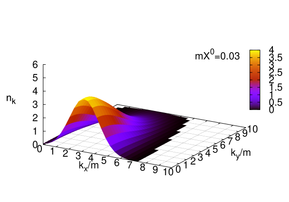
Figure 3: Initial distribution function $n_{\bf k}^{0}(mX^{0}=0.03)$. This function is plotted in $k_{x}-k_{y}$ momentum plane.

Now let us discuss the time evolution of the KB equation for the transverse modes. We solve (12a) and (12b) with mass $m^{2}$ and self-energy, which contains three transverse Green’s functions. Time evolution of Green’s functions is performed by referring to and in a similar way as Ref. Berges. We follow the evolution of $n_{\bf k}(X^{0})$ as a function of $\tilde{\omega}_{\bf p}$ defined as

$$n_{\bf k}(X^{0})+\frac{1}{2}= \left.\sqrt{F(\partial_{x^{0}}\partial_{y^{0}}F)-(\partial_{x^{0}}F)^{2}}\right|_{x^{0}=y^{0}=X^{0}}\ ,$$ (49)

$$\tilde{\omega}_{\bf k}(X^{0})= \left.\sqrt{(\partial_{x^{0}}\partial_{y^{0}}F)/F}\right|_{x^{0}=y^{0}=X^{0}}\ .$$ (50)

starting from the initial condition Eq. (48).

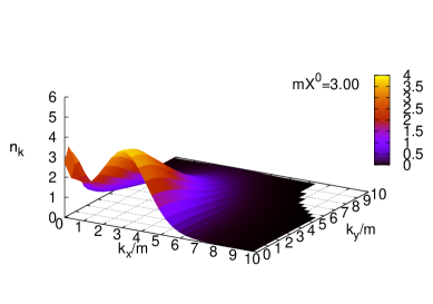
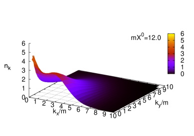
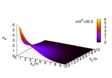
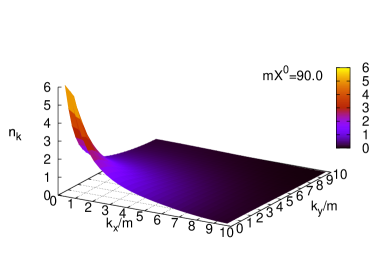
Figure 4: Number distribution function $n_{\bf k}$ at $mX^{0}=3.0$(upper left), $mX^{0}=12$ (upper right), $mX^{0}=30$(lower left) and $mX^{0}=90$ (lower right). The coupling constant and the number of color are $g^{2}/m=0.08$ and $N=3$.

In Fig. 4, we show the time evolution of $n_{\bf k}(X^{0})$ at $3.0\leq mX^{0}\leq 90$ with $g^{2}/m=0.08$ and $N=3$. In Fig. 5, we compare the number distribution $n_{\bf k}$ as a function of $\omega_{\bf k}$ in Case I and II. There are several points to be noted from these distribution. First, we find that the distribution function converges to the equilibrium distribution. At later times, the number distribution function loses its Gaussian structure and becomes isotropic in momentum space. Thus we have confirmed that off-shell transverse $g\leftrightarrow gg$ processes can cause kinetic equilibrium. Secondly, the equilibrium distribution at low energy is in agreement with the Bose distribution. At later times, the temperature and the chemical potential are found to be $T\simeq 2.8(3.2)$ and $\mu\simeq-1.7(-1.4)$ at $mX^{0}=120(174)$. The chemical potential appears to converge to zero as expected because the number of gluons is not a conserved variable. Simulations starting from different initial conditions with the same energy density show the same distributions at late times. Thirdly, high momentum modes are found to need longer time to grow up. For the modes with $\omega>6$, the distribution function is still different from the Bose distribution at $mX^{0}\sim 120$. Finally, we find that the results are almost the same for non-zero momentum modes in Cases I and II. The zero momentum mode of $n_{\bf k}(X^{0})$ in Case I remains the same value since zero momentum mode of the self-energy is always zero, but it can evolve in Case II and approaches the Bose distribution value at zero momentum. We can conclude that the ambiguities at ${\bf k},{\bf p},{\bf k}+{\bf p}=0$ does not induce any practical problems.

Figure 6 shows the time evolution of the entropy density $s^{0}/m^{2}$ (51) with $g^{2}/m=0.08$ and $0.06$. Here we employ another entropy density expression,

$$s^{0}(X)=(d-1)\int\!\!\frac{d^{d}k}{(2\pi)^{d}}\left[(1+n_{\bf k})\ln(1+n_{\bf k})-n_{\bf k}\ln n_{\bf k}\right],$$ (51)

which can be a criteria of thermalization,[52] instead of entropy density (27) to reduce numerical cost. The entropy density Eq. (51) is an approximate expression of Eq. (27), and it can be derived from (27) in the quasi-particle limit; by setting $\Sigma_{\rho}\rightarrow 0$, replacing $G^{12}=-i\rho f=2\pi\delta((k^{0})^{2}-\tilde{\omega}_{\bf k}^{2})(\theta(-k^{0})+n_{\bf k})$ and $G^{21}=-i\rho(1+f)=2\pi\delta((k^{0})^{2}-\tilde{\omega}_{\bf k}^{2})(\theta(k^{0})+n_{\bf k})$ as in Ref. Nishiyama and neglecting longitudinal part. Entropy density increases monotonically in the whole evolution. It increases rapidly at early times when the Gaussian structure collapses, and it saturates in the later stage when the kinetic equilibrium is nearly achieved. Monotonically increasing evolution is consistent with the H-theorem. Thus we confirm again that the leading order self-energy with off-shell processes, such as $g\leftrightarrow gg$, contributes to entropy production and equilibration in the numerical simulation without gradient expansion in the temporal axial gauge. This entropy production is characteristic in off-shell KB dynamics, since Boltzmann equation prohibits $g\leftrightarrow gg$. This property of off-shell effects may help the understanding of the early thermalization of dense nonequilibrium gluonic system in the initial stage of the heavy ion collision.

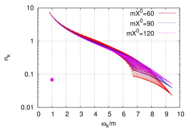
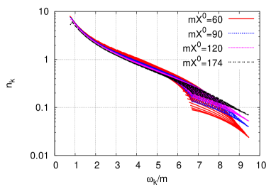
Figure 5: Logarithmic plot of number distribution function $n_{\bf k}$ at late times. Left and right panels show the results in Case I and Case II, respectively. In Case I, we show the zero momentum mode with the filled circle.

Before closing, we examine the energy conservation in the present numerical simulation. The total energy is given by

$$\epsilon_{tot} = \epsilon_{kin}+\epsilon_{pot}$$ (52)

$$\epsilon_{kin}/L^{d} = \frac{1}{2}\int\!\!\frac{d^{d}p}{(2\pi)^{d}}({\bf p}^{2}+m^{2}+\partial_{x^{0}}\partial_{y^{0}})F(x^{0},y^{0};{\bf p})\Big{|}_{x^{0}=y^{0}=X^{0}}$$ (53)

$$\epsilon_{pot}/L^{d} = \frac{1}{4}\int\!\!\frac{d^{d}p}{(2\pi)^{d}}I(X^{0},{\bf p})-\frac{1}{2}\int\!\!\frac{d^{d}p}{(2\pi)^{d}}{\rm Re}\Pi_{T,{\rm R};vac}F(X^{0},X^{0};{\bf p})$$

$$I(X^{0},{\bf p}) = \int_{0}^{X^{0}}\!\!dt^{\prime}\left[\Pi_{\rho}(X^{0},t^{\prime};{\bf p})F(t^{\prime},X^{0};{\bf p})-\Pi_{F}(X^{0},t^{\prime};{\bf p})\rho(t^{\prime},X^{0};{\bf p})\right]$$ (54)

as shown in Refs. Baym,JCG,AST,IKV2. Figure 7 shows the kinetic, potential and total energy as a function of time $X^{0}$ for $g^{2}/m=0.08$ measured from their initial values. We show the results relative to the initial total energy density, $\epsilon_{tot}/m\sim\epsilon_{kin}/m=18800$ in our lattice spacing. We find that the growth of the kinetic energy is cancelled by the decrease of potential energy, and that the energy error is within 0.5 percent. This is also true in Case I.

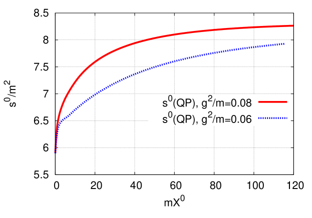
Figure 6: Evolution of entropy density in quasiparticle approximation (51) with $g^{2}/m=0.08$ (solid) and 0.06 (dotted).

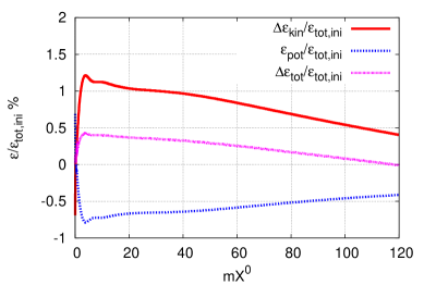
Figure 7: Evolution of kinetic (solid), potential (dotted) and total energy (bold solid) in units of m with $g^{2}/m=0.08$.

5 Summary

In this paper, first we have reviewed the Kadanoff-Baym (KB) dynamics for the non-Abelian gauge theory in the temporal axial gauge with the 2PI effective action. As an interaction, we have shown the form of leading order self-energy in KB equation. In the hard thermal loop (HTL) approximation, the leading order self-energy contributes to a mass shift (Debye mass or the thermal mass). Without the HTL approximation, nonlocal part of the self-energy couples two different momentum modes, and have a possibility to produce the width of the spectral function and change the number distribution function during the time evolution. By assuming that the system is spatially uniform and isotropic in the color space, we have decomposed the Fourier transformed Green’s function into the transverse and longitudinal components, and expressed the Schwinger-Dyson (SD) equation in the form of the KB equation, i.e. the coupled evolution equation of the spectral and statistical functions.

We have introduced the kinetic entropy current and given a proof of the H-theorem for the leading order self-energy. From this proof we find that nonlocal part of self-energy can induce entropy production. The entropy is produced via the off-shell processes such as $g\leftrightarrow gg$, and the transverse part of the entropy production, (TTT) in Eq. (LABEL:eq:TTT), is shown to stop increasing when the distribution function converges to the Bose-Einstein distribution.

Finally we have considered ’practical’ time evolution of the transverse modes of the KB equation numerically, as a first step of the non-equilibrium quantum field theoretical simulation of the non-Abelian gauge theory. We have approximated the local part of the self-energy by the constant mass term and the retarded local self-energy in vacuum, and the longitudinal part is ignored. We have evaluated the time evolution of this practical KB equation and investigated the equilibration of distribution functions. During the evolution, the number distribution function loses its initial information and approaches the Bose distributions. Off-shell particle number changing processes from the leading order self-energy are demonstrated to change the number distribution function in numerical simulation without gradient expansion. We have confirmed the entropy production from the off-shell processes. It is consistent with the proof of H-theorem.

The Kadanoff-Baym equation has a property that the width of the spectral function in the $p^{0}$ space and the memory effects allow off-shell collisions, which vary the momentum distribution of particle and induce entropy production. It is natural to think that these off-shell effects can contribute more rapid entropy production also in the 3+1 dimensions. This would be very important to investigate the entropy production in the heavy ion collisions. In order to apply the Kadanoff-Baym equation to actual heavy ion collision problems, it is necessary to include higher order effects in the coupling expansion, coupling with the color glass condensate (CGC) which appears as the classical field, and 3+1 dimensional numerical calculations. Works in these directions are in progress, and will be reported elsewhere.

References

- [1] I. Arsene et al. [BRAHMS Collaboration], Nucl. Phys. A 757 (2005), 1; K. Adcox et al. [PHENIX Collaboration], Nucl. Phys. A 757 (2005), 184; B. B. Back et al. [PHOBOS Collaboration], Nucl. Phys. A 757(2005), 28; J. Adams et al. [STAR Collaboration], Nucl. Phys. A 757 (2005), 102.
- [2] M. Gyulassy and L. McLerran, Nucl. Phys. A 750 (2005), 30.
- [3] U. W. Heinz and P. F. Kolb, Nucl. Phys. A702 (2002), 269; U. W. Heinz, AIP Conf. Proc. 739 (2005), 163.
- [4] T. Hirano, U. W. Heinz, D. Kharzeev, R. Lacey and Y. Nara, Phys. Lett. B 636 (2006), 299.
- [5] R. Baier, A. H. Nueller, D. Schiff and D. T. Son, Phys. Lett. B502 (2001), 51.
- [6] A. Ono, H. Horiuchi, T. Maruyama and A. Ohnishi, Prog. Theor. Phys. 87 (1992), 1185.
- [7] H. Sorge, Phys. Rev. C 52 (1995), 3291.
- [8] Y. Nara, N. Otuka, A. Ohnishi, K. Niita and S. Chiba, Phys. Rev. C 61 (2000), 024901.
- [9] P. K. Sahu, W. Cassing, U. Mosel and A. Ohnishi, Nucl. Phys. A 672 (2000), 376; P. Danielewicz, R. Lacey and W. G. Lynch, Science 298 (2002), 1592; M. Isse, A. Ohnishi, N. Otuka, P. K. Sahu and Y. Nara, Phys. Rev. C 72 (2005), 064908.
- [10] T. Hirano, M. Isse, Y. Nara, A. Ohnishi and K. Yoshino, Phys. Rev. C 72 (2005), 041901; P. K. Sahu, S. C. Phatak, A. Ohnishi, M. Isse and N. Otuka, Pramana 67 (2006), 257.
- [11] L. D. McLerran and R. Venugopalan, Phys. Rev. D 49 (1994), 2233.
- [12] P. Arnold, J. Lenaghan, G.D. Moore and L.G. Yaffe, Phys. Rev. Lett. 94 (2005), 072302.
- [13] A. Dumitru and Y. Nara, Phys. Lett. B 621 (2005) 89; A. Dumitru, Y. Nara and M. Strickland, Phys. Rev. D 75 (2007), 025016.
- [14] P. Romatschke and R. Venugopalan, Phys. Rev. Lett. 96 (2006), 062302; Phys. Rev. D 74 (2006), 045011.
- [15] T. Kunihiro, B. Muller, A. Ohnishi and A. Schafer, Prog. Theor. Phys. 121 (2009), 555; T. Kunihiro, B. Muller, A. Ohnishi, A. Schafer, T. T. Takahashi and A. Yamamoto, arXiv:1008.1156 [hep-ph].
- [16] S. Mrowczynski, Phys. Lett. B314 (1993), 118; Phys. Rev. C 49 (1994), 2191; Phys. Lett. B 393 (1997), 26; PoS CPOD2006 (2006), 042.
-
[17]
A. Iwazaki, Phys. Rev. C 77 (2008), 034907;
H. Fujii and K. Itakura, Nucl. Phys. A 809 (2008), 88. - [18] J. Berges, AIP Conf. Proc. 739 (2005), 3 [hep-ph/0409233].
- [19] J. Berges and J. Serreau, 6th Conference on Strong and Electroweak Matter 2004 (SEWM04), Helsinki, Finland, 16-19 Jun 2004, [hep-ph 0410330].
- [20] G. Baym and L. Kadanoff, Phys. Rev. 124 (1961), 287.
- [21] L.P. Kadanoff, G. Baym, Quantum Statistical Mechanics (Benjamin, New York, 1962).
- [22] J. Luttinger and J. Ward, Phys. Rev. 118 (1960), 1417.
- [23] G. Baym, Phys. Rev. 127 (1962), 1391.
- [24] J. Schwinger, J. Math. Phys. 2 (1961), 407.
- [25] L.V. Keldysh, ZHETF 47 (1964), 1515 [Sov. Phys. JETP 20 (1965), 235].
- [26] J. M. Cornwall, R. Jackiw and E. Tomboulis, Phys. Rev. D 10 (1974), 2428.
- [27] A.J. Niemi and G.W. Semenoff, Ann. Phys. 152 (1984), 105; Nucl. Phys. B 230 (1984), 181.
- [28] E. Calzetta, B.L. Hu, Phys. Rev. D 37 (1988), 2878.
- [29] J. Berges and J. Serreau, Phys. Rev. Lett. 91 (2003), 111601.
- [30] G. Aarts and A. Tranberg, Phys. Rev. D 77 (2008), 123521; Phys. Rev. D 77 (2008), 123521.
- [31] A. Tranberg, JHEP 0811 (2008), 037; A. Tranberg, Nucl. Phys A 820 (2009), 195C-198C.
- [32] A. Arrizabalaga, J. Smit and A. Tranberg, JHEP 0410 (2004), 017.
- [33] N.M. Hugenholtz and D. Pines, Phys. Rev. 116 (1959), 489.
- [34] H. Van Hees and J. Knoll, Phys. Rev. D 66 (2002), 025028.
- [35] J. Berges, S. Borsnyi and C. Wetterich, Phys. Rev. Lett. 93 (2004), 142002.
- [36] P. Danielewicz, Ann. Phys. (N.Y.) 152 (1984), 305.
- [37] G. Aarts and J. Berges, Phys. Rev. D 64 (2001), 105010.
- [38] J. Berges and J. Cox, Phys .Lett. B 517 (2001), 369.
- [39] S. Juchem, W. Cassing and C. Greiner, Phys. Rev. D 69 (2004), 025006.
- [40] A. Arrinzabalaga, J. Smit and A. Tranberg, Phys. Rev. D 72 (2005), 025014.
- [41] M. Lindner and M. M. Müller; Phys. Rev. D 73 (2006), 125002.
- [42] F. Cooper, J.F. Dawson and B. Mihaila, Phys. Rev. D 67 (2003), 056003.
- [43] G. Aarts, D. Ahrensmeier, R. Baier, J. Berges and J. Serreau, Phys. Rev. D 66 (2002), 045008.
- [44] J. Berges, Nucl. Phys. A 699 (2002), 847.
- [45] A. Arrizabalaga and J. Smit, Phys. Rev. D 66 (2002), 065014.
- [46] M.E. Carrington, G. Kunstatter and H. Zaraket, Eur. Phys. J C 42 (2005), 253.
- [47] K. Kajantie and J. Kapusta, Ann. Phys. 160 (1985), 477.
- [48] Z. Xu and C. Greiner, Phys. Rev. C 71 (2005), 064901; Phys. Rev. C 76 (2007), 024911.
- [49] J. Berges, S. Scheffler and D. Sexty, Phys. Rev. D 77 (2008), 034504; Prog. Part. Nucl. Phys. 61 (2008), 86; J. Berges, D. Gelfand, S. Scheffler, D. Sexty, Phys. Lett. B677 (2009), 210.
- [50] Y.B. Ivanov, J. Knoll, and D.N. Voskresensky, Nucl. Phys. A672 (2000), 313.
- [51] T. Kita, J. Phys. Soc. Jpn. 75 (2006), 114005.
- [52] A. Nishiyama, Nucl. Phys. A 832 (2010), 289.
- [53] A. Nishiyama and A. Ohnishi, arXiv:1006.1124 [nucl-th].
- [54] J.P. Blaizot and E. Iancu, Phys. Rep. 359 (2002), 355.
- [55] J. P. Blaizot, E. Iancu and A. Rebhan, Phys. Rev. Lett. 83 (1999), 2906; Phys. Lett. B 470 (1999), 181.
- [56] J. P. Blaizot, E. Iancu and A. Rebhan, Phys. Rev. D 63 (2001), 065003.
- [57] E. Riedel, Z. Phys. 210 (1968), 403.
- [58] B. Vanderheyden and G. Baym, J. Stat. Phys. 93 (1998), 843.
- [59] G. M. Carneiro and C. J. Pethick, Phys. Rev. B 11 (1975), 1106.
- [60] I. Montvay and G. Münster; Quantum Fields on a Lattice, Cambridge University Press (1994).
- [61] Y.B. Ivanov, J. Knoll, and D.N. Voskresensky, Ann. Phys. 293 (2001), 126.