Correlation induced non-Abelian quantum holonomies

Abstract

In the context of two-particle interferometry, we construct a parallel transport condition that is based on the maximization of coincidence intensity with respect to local unitary operations on one of the subsystems. The dependence on correlation is investigated and it is found that the holonomy group is generally non-Abelian, but Abelian for uncorrelated systems. It is found that our framework contains the Lévay geometric phase [2004 J. Phys. A: Math. Gen. 37 1821] in the case of two-qubit systems undergoing local $SU(2)$ evolutions.

1 Introduction

The theory of holonomies and geometric phases associated with evolutions of a quantum system is by now a well developed subject. The initial work by Berry [1] on the Abelian geometric phase of adiabatic evolutions of non-degenerate states has been extended in many directions, to include non-adiabatic evolutions [2] as well as non-Abelian holonomies of sets of degenerate states [3, 4], and to mixed states [5]. It was subsequently discovered that the quantum geometric phase had an early counterpart in the geometric phase discovered by Pancharatnam in the context of classical optics [6, 7, 8]. The Pancharatnam construction has been generalized to the non-Abelian case by utilizing subspaces [9, 10, 11, 12]. More recently holonomies that bear a relation to correlations have been constructed in the context of multipartite and lattice systems [13, 14, 15, 16].

The idea of this paper is to develop the concept of geometric phases in another direction and use two-particle interferometry to construct correlation induced non-Abelian holonomies in a way that does not depend on degeneracy, but on the ability to divide the system into spatially separated subsystems. Instead of considering parallel transport of subspaces, we consider the natural tensor product structure of a bipartite state, induced by the spatial separation of the two subsystems, and local unitary operations to define the parallel transport.

The parallel transport condition to be introduced is similar to that of the Pancharatnam construction [6, 7, 8], in which two states $\mid\!{A}\rangle$ and $\mid\!{B}\rangle$ of a quantum system are defined to be in-phase if their scalar product $\langle{B}\!\mid\!{A}\rangle$ is a positive number. This condition can be implemented in a Mach-Zehnder interferometric setup, where the spatial state of the system prior to the last beam splitter is a coherent superposition of the two paths [17, 18]. If we let $\mid\!{A}\rangle$ and $\mid\!{B}\rangle$ be the internal states corresponding to the output of respective paths of the interferometer, then Pancharatnam parallelity is achieved by shifting a $U(1)$ phase in one of the paths, such that the interference intensity is maximal.

In two-particle interferometry [19, 20, 21] the spatial state of the two-particle system is a coherent superposition of two distinct pairs of correlated paths for the two subsystems. In the same spirit as Pancharatnam we use a two-particle interferometric intensity, namely the coincidence intensity in a Franson interferometer [20, 21, 22], to define an ”in-phase” condition and the corresponding parallel transport. An arbitrary unitary operation is performed in one of the arms of the interferometer on the first subsystem, thus making the outputs of the two possible pairs of paths different. Subsequently, another unitary operation is performed in the other arm on the second subsystem, and is chosen such as to achieve maximal coincidence intensity. This second unitary is considered to be the ”phase” degree of freedom of the system and at maximal intensity the two outputs are considered to be ”in-phase”, or ”parallel”. Thus we consider the orbit space formed by the state space of the system modulo this unitary degree of freedom on the second subsystem to be the space in which the system is parallel transported.

In the special case of pure two-qubit states, and evolutions generated by local $SU(2)$ operations, the state space naturally fibrates through the second Hopf fibration and the orbit space of the two qubit-states can be mapped to the state space of a quaternionic qubit [23]. The coincidence intensity of the Franson interferometer, in this case, corresponds to the quaternionic quantum mechanics analogue of the Mach-Zehnder intensity and the associated parallel transport condition corresponds to the Lévay connection [24] restricted to local $SU(2)$ evolutions.

The outline of the paper is as follows. It turns out that the Stokes tensor formalism [25] is convenient for our analysis. Therefore we briefly review this representation in section 2. Section 3 contains a description of the Franson interferometric setup and we define the parallelity condition in this setting. In section 4, we describe the parallel transport procedure, discuss the properties of the related holonomy group and introduce the corresponding connection form. Finally, in section 5 we consider the parallel transport scheme in the special case of pure two-qubit states, and evolutions generated by $SU(2)$ operations and its relation to the quaternionic representation of pure two-qubit states and the corresponding Lévay connection. The paper ends with the conclusions.

2 Stokes tensor formalism

In the Stokes tensor formalism [25], single particle quantum states are represented as real vectors and $N$-partite states are represented as real $N$-tensors. A multi-partite system consisting of parts $A,B,\dots{Z}$, where part $K$ has dimension $D_{K}$, is represented as a $D_{A}^{2}\times{D_{B}^{2}}\times\dots\times{D_{Z}^{2}}$-dimensional tensor $S_{j_{A}j_{B}\dots{j}_{Z}}$. This tensor is related to the density matrix representation $\hat{\rho}$ of the same state as

$$\hat{\rho}=\!\!\sum_{j_{A}=0}^{D_{A}^{2}-1}\!\sum_{j_{B}=0}^{D_{B}^{2}-1}\!\!\dots\!\!\sum_{j_{Z}=0}^{D_{Z}^{2}-1}\!\!\left[\prod_{K=A}^{Z}\frac{1}{\delta_{0j_{K}}\!(D_{K}\!-2)\!+\!2}\right]\!\!S_{j_{A}j_{B}\ldots j_{Z}}\hat{\chi}^{A}_{j_{A}}\!\otimes\!\hat{\chi}^{B}_{j_{B}}\!\otimes\!\dots\!\otimes\!\hat{\chi}^{Z}_{j_{Z}},$$

where $\hat{\chi}^{K}_{0}\equiv{\hat{1}^{K}}$ and $\hat{\chi}^{K}_{j_{K}}$ $(j_{K}=1,2,...,D_{K}^{2}-1)$ are the $D_{K}^{2}-1$ traceless generators of $U(D_{K})$ operations on system $K$. In the following, we shall in most cases use the simplifying notation $\hat{\chi}_{j}^{K}$ for the generators on subsystem $K$. The Hermitean, traceless and linearly independent generators $\{\chi_{j}^{K}\}_{j=1}^{D^{2}_{K}-1}$ of $U(D_{K})$ satisfy orthogonality $\Tr(\hat{\chi}_{j}^{K}\hat{\chi}_{k}^{K})=2\delta_{jk}$, and $[\hat{\chi}_{k}^{K},\hat{\chi}_{l}^{K}]=2i\sum_{m=1}^{D^{2}_{K}-1}f_{klm}\hat{\chi}^{K}_{m}$ as well as $\{\hat{\chi}^{K}_{k},\hat{\chi}^{K}_{l}\}=\frac{4}{D_{K}}\delta_{kl}\hat{1}^{K}+2\sum_{n=1}^{D^{2}_{K}-1}d_{kln}\hat{\chi}^{K}_{n}$, where $d_{jkl}$ and $f_{jkl}$ are the symmetric and antisymmetric structure constants, respectively, of $U(D_{K})$. The factors $\left[\delta_{0j_{K}}(D_{K}-2)+2\right]^{-1}$ are inserted so that $S_{j_{A}j_{B}\ldots j_{Z}}=\Tr\left(\hat{\rho}\hat{\chi}^{A}_{j_{A}}\!\otimes\!\hat{\chi}^{B}_{j_{B}}\!\otimes\!\dots\!\otimes\!\hat{\chi}^{Z}_{j_{Z}}\right)$.

We shall represent unitary operators $U(D_{K})$ on a form compatible with this formalism. These are represented by complex vectors with elements $U_{j}=\frac{1}{[\delta_{0j}(D_{K}-2)+2]}\Tr(\hat{U}\hat{\chi}_{j}^{K})$ so that

$$\hat{U}=\sum_{j=0}^{D_{K}^{2}-1}U_{j}\hat{\chi}^{K}_{j}.$$ (2)

Unitarity of the operators demand that $\{U_{j}\}$ are complex numbers satisfying

$$\mid\!{U_{0}}\!\mid^{2}+\frac{2}{D_{K}}\sum_{j=1}^{D_{K}^{2}-1}\!\mid\!{U_{j}}\!\mid^{2}=1$$ (3)

and

$$\sum_{j,k=0}^{D_{K}^{2}-1}U_{j}U_{k}^{\ast}\left[d_{jkl}+if_{jkl}+(\delta_{j0}\delta_{kl}+\delta_{k0}\delta_{jl})\right]=0$$ (4)

for each $1\leq{l}\leq{D_{K}^{2}-1}$.

In this paper we focus on bipartite systems $A+B$ and therefore it can be instructive to consider some general properties of the Stokes 2-tensor. The zeroth row and zeroth column of the tensor, with elements $S_{0j}$ and $S_{j0}$ respectively, are the Stokes 1-tensors corresponding to the reduced states of subsystem $A$ and $B$, and these contain all the local information of the bipartite system. The remaining part, formed by the elements $S_{ij},\phantom{u}i,j>0$, contains all the correlations of the state and this subtensor, the correlation matrix, is denoted by $M_{ij}$. This matrix has previously been used to study correlations and separability in quantum systems [26, 27].

A unitary transformation on subsystem $A$ transforms the reduced density matrix as $\hat{U}\hat{\rho}^{A}\hat{U}^{\dagger}$. This corresponds to a transformation $RS$, on $S$ where $R_{jk}=\frac{1}{((D_{A}-2)\delta_{j0}+2)}\Tr(\hat{U}\hat{\chi}^{A}_{k}\hat{U}^{\dagger}\hat{\chi}^{A}_{j})$. The $R$ matrix is an orthogonal matrix, as can be seen by observing that

$$\delta_{jk}\!\! = \!\!\frac{1}{[(D_{A}\!-\!2)\delta_{j0}\!+\!2]}\!\Tr(\hat{\chi}^{A}_{j}\hat{\chi}^{A}_{k})=\frac{1}{[(D_{A}\!-\!2)\delta_{j0}\!+\!2]}\!\Tr(\hat{U}\hat{\chi}^{A}_{j}\hat{U}^{\dagger}\hat{U}\hat{\chi}^{A}_{k}\hat{U}^{\dagger})=$$

$$= \frac{1}{[(D_{A}\!-\!2)\delta_{k0}\!+\!2][(D_{A}\!-\!2)\delta_{j0}\!+\!2]}\!\!\sum_{l=0}^{D_{A}^{2}-1}\!(U\chi_{j}^{A}U^{\dagger})_{l}(U\chi_{k}^{A}U^{\dagger})_{l}=\!\!\sum_{l=0}^{D_{A}^{2}-1}\!\!R^{T}_{jl}R_{lk}.$$

Similarly a unitary transformation on subsystem $B$ corresponds to an orthogonal matrix acting on $S$ from the right. It should be noted that the $M$ matrix transforms under local unitary operations on subsystem $A$ and $B$ through left and right action, respectively, by orthogonal matrices.

As an example of how the $M$ matrix behaves we can consider a pure two-qubit state in the Schmidt basis

$$\mid\!\psi\rangle=a\!\mid\!{00}\rangle+b\!\mid\!{11}\rangle$$ (6)

where $a$ and $b$ are real non-negative numbers and $a^{2}+b^{2}=1$. Expressed in the Schmidt basis, the correlation matrix with elements $M_{jk}=\Tr\left(\hat{\rho}\hat{\sigma}_{j}^{A}\!\otimes\!\hat{\sigma}_{k}^{B}\right)$, $\sigma_{j}^{A}$ and $\sigma_{k}^{B}$, $j,k=1,2,3$, being the standard Pauli operators on subsystem $A$ and $B$, respectively, reads

$$M=\left(\begin{array}[]{ccc}C&0&0\\ 0&-C&0\\ 0&0&1\end{array}\right),$$ (10)

where $C=2ab$ is the pure state concurrence [28]. Here it is clearly seen that $M$ is rank one for product states. It must be emphasized that $M_{11}=-M_{22}=C$ because we choose $a,b\in\mathbb{R}$. The elements of $M$ are not explicit functions of concurrence for arbitrary complex coefficients $a,b$. However, since all pure two-qubit states with the same concurrence can be related by local unitaries, corresponding to orthogonal transformations acting from the right and the left on $M$, the absolute value of the determinant of $M$

$$\mid\!\det{M}\!\mid=C^{2}$$ (11)

is invariant under local unitary transformations and measures concurrence. For maximally entangled states we thus have that $\mid\!\!\det{M}\!\!\mid=1$.

When we consider mixed states there can be correlations also in separable states. As an example of how the $M$ matrix registers correlation for mixed states we can consider the Werner states [29]

$$\hat{\rho}_{W}=p\mid\!\psi\rangle\langle\psi\!\mid+\frac{(1-p)}{4}\hat{1}^{A}\!\otimes\hat{1}^{B},$$ (12)

where $\mid\!\!\psi\rangle$ is some maximally entangled state and $p\in[0,1]$. The absolute value of the determinant is $\mid\!\det{{M}}\!\mid=p^{3}$, which can be compared to the square of the concurrence $C=\max\left[\frac{(3p-1)}{2},0\right]$. Thus for $p\leq{\frac{1}{3}}$ the determinant of $M$ is nonzero even though the state is separable. This underscores that the $M$ matrix for mixed states is sensitive to correlations in general.

3 Parallel transport condition

3.1 Interferometric setup and parallelity

A Franson interferometer [20, 21, 22],is a two-particle device composed of two identical unbalanced two-path interferometers, so-called Franson loops, as shown in Fig. 1. The two parts of the bipartite state are emitted, one into each Franson loop. A beam splitter divides each path in two different paths of unequal length, which later converge at a second beam splitter. The difference in path length between the two arms in each Franson loop is chosen to be the same, and such that the difference in transit time $\Delta{t}$ is greater than the single particle coherence time. The transit time difference between the paths must be smaller than the coherence time of the bipartite state to allow two-particle interference. Of importance is that the emitter is such that is impossible to define a time of emission. Detectors are placed after the convergence of the two paths in each Franson loop and coincidence measurements are made.

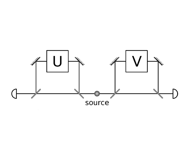
Figure 1: The Franson interferometer setup. Unitary operations on the internal degrees of freedom the particle are performed in the long arms of each Franson loop.

Since we discard non-coincidental detections, corresponding to the bipartite system traversing a long path in one of the Franson loops and a short path in the other, it is necessary that the time resolution of the detectors is smaller than $\Delta{t}$. Furthermore, due to the requirement that time of emission cannot be defined, and since no measurements are made inside the Franson loops, it cannot be ascribed to a coincidence detection event that the bipartite system traversed either the two short paths or the two long ones. Hence the system is in a coherent superposition of having traversed the two long arms, and having traversed the two short arms. In the long paths of each sub-interferometer we place devices that perform unitary operations on the internal state of the bipartite state. After the point of convergence of the two paths, the effective unnormalized internal state is under the above requirements therefore

$$\hat{\rho}=\frac{1}{4}(\hat{1}+\hat{U}\!\otimes\!\hat{V})\hat{\rho}_{0}(\hat{1}+\hat{U}^{\dagger}\!\otimes\!\hat{V}^{\dagger}),$$ (13)

where $\hat{\rho}_{0}$ is the initial internal state. Given $\hat{U}=\sum_{j=0}^{D_{A}^{2}-1}U_{j}\hat{\chi}_{j}^{A}$, and $\hat{V}=\sum_{j=0}^{D_{B}^{2}-1}V_{j}\hat{\chi}_{j}^{B}$ where $\hat{\chi}_{j}^{A}$ and $\hat{\chi}_{j}^{B}$ are the generators of $U(D_{A})$ and $U(D_{B})$, respectively, the coincidence detection intensity $I^{AB}$ is

$$I^{AB}={\frac{1}{2}+\frac{1}{2}\mathrm{Re}\Tr(\hat{U}\otimes\hat{V}\hat{\rho}_{0})}.$$ (14)

The coincidence detection intensity $I^{AB}$, henceforth referred to simply as ”intensity”, is the ratio between the measured intensity for a given $\hat{U}$ and $\hat{V}$, and the intensity measured if $\hat{U}=\hat{V}=\hat{1}$. The expression for $I^{AB}$ in the Stokes tensor formalism is

$$I^{AB}=\frac{1}{2}+\frac{1}{2}\!\sum_{k=0}^{D_{A}^{2}-1}\sum_{j=0}^{D_{B}^{2}-1}\mathrm{Re}(V_{j}U_{k})S_{kj},$$ (15)

where the second term is the interference term.

We now define the parallelity condition in the Franson setup for a bipartite system consisting of two qudits of dimension $D_{A}$ and $D_{B}$. We ask, given that a specific unitary operation $\hat{U}\in{U(D_{A})}$ has been chosen in the first Franson loop, what unitary operation $\hat{V}\in{U(D_{B})}$ should be chosen in the second Franson loop in order to maximize the coincidence intensity? We take maximal coincidence intensity as the definition of parallelity between the output of the two short paths and the output of the two long paths. This maximization procedure is the analogue of the procedure used to define Pancharatnam parallelity in the context of a Mach-Zehnder interferometer [17, 18], but here the Franson coincidence intensity has taken the role of the Mach-Zehnder intensity and $\hat{V}$ has taken the role of the $U(1)$ phase factor. It should be noted that if $S$ does not have full rank, then there exist $\hat{U}$ such that $\sum_{k=0}^{D_{A}^{2}-1}U_{k}S_{kj}=0$ for all $j$. In this case the interference term is identically zero for all $\hat{V}$, but if $\sum_{k=0}^{D_{A}^{2}-1}U_{k}S_{kj}\neq 0$ there will always be a $\hat{V}$ corresponding to maximal intensity.

To find a formal expression for the operator $\hat{V}$ that maximizes the intensity, we seek to maximize $I^{AB}$ in equation (15) with respect to the coefficients $V_{k}$, using Lagrange’s method. To enforce unitarity of $\hat{V}$ we introduce the constraints $\mid\!\!{V}_{0}\!\!\mid^{2}+\frac{2}{D_{B}}\sum_{j=1}^{D_{B}^{2}-1}\mid\!\!{V}_{j}\!\!\mid^{2}=1$ and $\sum_{j,k=0}^{D_{B}^{2}-1}V_{j}V_{k}^{\ast}\left[d_{jkl}+if_{jkl}+(\delta_{j0}\delta_{kl}+\delta_{k0}\delta_{jl})\right]=0$ for each $1\leq{l}\leq{D_{B}^{2}-1}$. We thus construct the auxiliary function $f(\{V_{j}\},\{V_{j}^{*}\})$, that is to be extremized, as

$$f\!\left(\{V_{j}\},\{V_{j}^{*}\}\right)=\sum_{k=0}^{D_{A}^{2}-1}\sum_{j=0}^{D_{B}^{2}-1}(V_{j}U_{k}+V_{j}^{*}U_{k}^{*})S_{jk}$$

$$-\lambda\!\!\left(V_{0}V_{0}^{*}+\frac{2}{D_{B}}\sum_{j=1}^{D_{B}^{2}-1}V_{j}V_{j}^{*}-1\right)$$

$$-\sum_{l=1}^{D_{B}^{2}-1}\mu_{l}\sum_{j,k=0}^{D_{B}^{2}-1}V_{j}V_{k}^{\ast}\left[d_{jkl}+if_{jkl}+(\delta_{j0}\delta_{kl}+\delta_{k0}\delta_{jl})\right].$$

Using Lagrange’s method we seek the points were the gradient of the auxiliary function with respect to the variables $V_{j}$ and $V_{j}^{*}$ vanishes. The components $V_{k}$ defining these points satisfy the equations

$${\lambda}\!\left[\frac{2}{D_{B}}\!-\!\!\left(1\!-\!\frac{2}{D_{B}}\right)\!\delta_{k0}\right]\!\!{V_{k}}+\!\!\sum_{l=1}^{D_{B}^{2}-1}\!\!\mu_{l}\!\!\left[\!(\delta_{kl}V_{0}+\delta_{k0}V_{l})+\!\!\sum_{j=1}^{D_{B}^{2}-1}\!\!V_{j}(d_{jkl}+if_{jkl})\!\right]\!\!\!=$$

$$=-\!\sum_{j=0}^{D_{A}^{2}-1}\!U_{j}^{*}S_{jk},\phantom{yuyuyuyuy}0\leq{k}\leq{D_{B}^{2}-1}.$$ (17)

If the coefficients $U_{j}$ are ordered as a $D_{A}^{2}$-dimensional vector $\bar{u}$ and likewise the coefficients $V_{k}$ are ordered as a $D_{B}^{2}$-dimensional vector $\bar{v}$, the above equations can be reexpressed as a matrix equation

$$B\bar{v}=-S^{T}\bar{u}^{\ast},$$ (18)

where $B$ is a $\lambda$ and $\mu_{l}$ dependent Hermitean matrix, given by

$$B_{kl}=\lambda\!\!\left[\frac{2}{D_{B}}\delta_{kl}-\!\left(1-\frac{2}{D_{B}}\right)\!\delta_{l0}\delta_{k0}\right]+\!\!\sum_{j=1}^{D_{B}^{2}-1}\!\mu_{j}(\delta_{jk}\delta_{l0}+\delta_{jl}\delta_{0k}+d_{jlk}-if_{jkl}).$$

Provided $B(\lambda,\bar{\mu})$ is invertible, the formal solution for $\hat{V}$ can be given as

$$\hat{V}=\sum_{l,k,j=0}^{D^{2}_{B}-1}B^{-1}_{lk}(\lambda,\bar{\mu})S^{T}_{kj}U_{j}^{\ast}\hat{\chi}^{B}_{l},$$ (20)

where $\bar{\mu}\equiv\!\{\mu_{j}\}$. The explicit form of the Lagrange parameters, and thus $B^{-1}$, is found by solving for the unitarity constraints on $\hat{V}$. The solutions of these constraint equations give us the critical points of the intensity as a function of $\hat{U}$. We can see from the constraints that for each solution $\lambda,\bar{\mu}$ there is a solution $-\lambda,-\bar{\mu}$ and if one of them corresponds to a local maximum, the other corresponds to a local minimum. There will be a unique solution to the maximization problem if and only if there is a unique global maximum of the intensity as a function of $\hat{U}$, corresponding to a combination of parameters $\lambda,\bar{\mu}$ satisfying the constraints.

In the general case, finding this solution as a function of $\hat{U}$ appears to be a non-trivial problem. For product states, however, the unitary $\hat{V}$ that maximizes the intensity is easily found and is always a Abelian $U(1)$ phase factor. This can be seen by observing that for product states $\rho^{A}\!\otimes\!\rho^{B}$ the coincidence intensity is

$$I^{AB}={\frac{1}{2}+\frac{1}{2}\mathrm{Re}\Tr(\hat{U}\hat{\rho}^{A})\Tr(\hat{V}\hat{\rho}^{B})}.$$ (21)

and therefore the $\hat{V}$ that maximizes this expression is found to be $\hat{V}=e^{-i\arg({\Tr(\hat{U}\hat{\rho}^{A})})}\hat{1}$. We may note that for the trivial case where $\hat{U}=e^{i\phi}\hat{1}$, we see that the intensity is maximal if and only if $\hat{V}=e^{-i\phi}\hat{1}$, regardless of the state of the bipartite system.

3.2 Example I: Qudit-qubit

In section 3.1, the solution $\hat{V}\in{U(D_{B})}$ to the maximization problem is not given on a closed form and it is not apparent how to find it. However, for the case where the second subsystem is a qubit, and therefore $\hat{V}\in{U(2)}$, the $B$ matrix is $B_{kl}={\lambda}\delta_{lk}+\sum_{j=1}^{3}\mu_{j}\left[(\delta_{jk}\delta_{l0}+\delta_{jl}\delta_{k0})-if_{jkl}\right]$. It can be seen that $B$ now separates as $B=\lambda\hat{1}+H$, where $H$ is Hermitean and $H^{2}\propto\hat{1}$, and therefore $B^{-1}=\frac{1}{\sqrt{\det{B}}}(-\lambda\hat{1}+H)$. Explicitly

$$B^{-1} = \frac{1}{\sqrt{\det{B}}}\left(\begin{array}[]{cccc}-{\lambda}&\mu_{1}&\mu_{2}&\mu_{3}\\ \mu_{1}&-\lambda&-i\mu_{3}&i\mu_{2}\\ \mu_{2}&i\mu_{3}&-{\lambda}&-i\mu_{1}\\ \mu_{3}&-i\mu_{2}&i\mu_{1}&-{\lambda}\end{array}\right),$$ (26)

$$\det{B} = \left(-\lambda^{2}+\bar{\mu}\cdot\bar{\mu}\right)^{2}.$$ (27)

While it is still not obvious how to find the Lagrange parameters in general we may solve it in some special cases. To illustrate this, let us consider a $\hat{U}$ that has the form $\hat{U}=U_{1}\hat{\sigma}_{1}+U_{2}\hat{\sigma}_{2}$, where $\hat{\sigma}_{1}$ and $\hat{\sigma}_{2}$ are the standard Pauli operators, and a pure state

$$\mid\!\psi\rangle=a\!\mid\!{00}\rangle+b\!\mid\!{11}\rangle,$$ (28)

where $a,b\geq{0}$. As a consequence of our choice of basis $S_{10}=S_{20}=0$ and the concurrence $C=2ab$. This together with our special choice of $\hat{U}$, implies that the intensity is

$$I^{AB}=\frac{1}{2}+\frac{C}{2}\mathrm{Re}(V_{1}U_{1}-V_{2}U_{2}).$$ (29)

Using equations (20) and (27), and the constraints, we find that $\bar{\mu}=0,\lambda=\pm{C}$, where the positive sign corresponds to the global maximum while the negative sign corresponds to the global minimum. The unitary operator $\hat{V}$ corresponding to the maximum is

$$\hat{V}=U_{1}^{*}\hat{\sigma}_{1}-U_{2}^{*}\hat{\sigma}_{2},$$ (30)

and the maximal intensity is

$$I^{AB}_{max}=\frac{1}{2}(1+{C}).$$ (31)

3.3 Example II: Restriction to $SU(D)$

A variation of the maximization procedure is to restrict the set from which $\hat{U}$ and $\hat{V}$ can be chosen. One natural restriction would be to consider only $SU(D_{A})$ and $SU(D_{B})$ operations in the Franson loops. When this restriction is made the qualitative properties of the parallel transport may change. It is for example no longer obvious that the unitaries $\hat{V}$ associated to a product state, will be a commuting set in the general case. The restriction where the second subsystem is a qubit and therefore $\hat{V}\in{SU(2)}$, however, leads to a significant simplification of the maximization problem. Here, we solve this problem and in particular show that product states are indeed associated with commuting sets of unitaries.

Since $SU(2)$ can be parametrized by four real numbers subject to only one constraint, the solution of the maximization problem can be found easily for arbitrary states and arbitrary $\hat{U}\in{SU(D_{A})}$. We choose the parametrization of $\hat{V}$ such that $V_{0}$ is real and $iV_{1},iV_{2},iV_{3}$ are purely imaginary. The intensity in this parametrization is

$$I^{AB}=\frac{1}{2}+\frac{1}{4}\left[\sum_{j=0}^{D_{A}^{2}-1}V_{0}(U_{j}+U_{j}^{*})S_{j0}+i\sum_{j=0}^{D_{A}^{2}-1}\sum_{k=1}^{3}V_{k}(U_{j}-U_{j}^{*})S_{jk}\right]$$ (32)

and $\hat{V}$ is found to be

$$\hat{V}=\frac{1}{2\lambda}\left[\sum_{j=0}^{D_{A}^{2}-1}(U_{j}+U_{j}^{*})S_{j0}\hat{1}^{B}+i\sum_{j=0}^{D_{A}^{2}-1}\sum_{k=1}^{3}(U_{j}-U_{j}^{*})S_{jk}\hat{\sigma}^{B}_{k}\right],$$ (33)

where $\hat{\sigma}^{B}_{m}$ are the Pauli operators. The remaining Lagrange parameter $\lambda$ is found from the unitarity condition $\sum_{j=0}^{3}\mid\!{V_{j}}\!\mid^{2}=1$ and is

$$\lambda=\pm\frac{1}{2}\sqrt{\left[\sum_{j=0}^{D_{A}^{2}-1}(U_{j}+U_{j}^{*})S_{j0}\right]^{2}+\sum_{k=1}^{3}\left[\sum_{j=0}^{D_{A}^{2}-1}(U_{j}-U_{j}^{*})S_{jk}\right]^{2}}.$$ (34)

The sign of $\lambda$ must be chosen positive since the trivial case $\hat{U}=\hat{1}$ implies $\hat{V}=\hat{1}$.

When the bipartite state is a product state $\hat{\rho}=\hat{\rho}^{A}\!\otimes\!\hat{\rho}^{B}$ we find that $\hat{V}=\frac{1}{2\lambda}[\sum_{j=0}^{D_{A}^{2}-1}(U_{j}+U_{j}^{*})S_{j0}\hat{1}^{B}+2i\sum_{j=0}^{D_{A}^{2}-1}(U_{j}-U_{j}^{*})S_{j0}(\hat{\rho}^{B}-\hat{1}^{B})]$. Hence for product states the unitary $\hat{V}$ that maximizes intensity commutes with $\hat{\rho}^{B}$ for any $\hat{U}$. Therefore the set of unitaries $\hat{V}$ associated to a product state commute with the density operator and with each other. The signature of a product state is thus that the corresponding set of unitaries will be commuting when the unitary operators on the second subsystem are restricted to $SU(2)$.

3.4 Example III: SO(D) and two-redit states

Another variation of of our procedure is to maximize the intensity for $\hat{V}\in{SO(D_{B})}$ given $\hat{U}\in{SO(D_{A})}$ in the other Franson loop. Since $SO(D)$ is the endomorphism group of the $D$-dimensional redit state space we may consider this restriction of the maximization procedure when the state space is restricted to a two-redit subspace. For two redits the state $\hat{\rho}$ naturally decomposes as

$$\hat{\rho}=\frac{1}{[\delta_{k0}(\!D_{A}\!-\!2)\!+\!2][\delta_{l0}(\!D_{B}\!-\!2)\!+\!2]}\sum_{k=0}^{D_{A}^{2}-1}\!\sum_{l=0}^{D_{B}^{2}-1}\!\left(S^{sym}_{kl}+S^{anti-sym}_{kl}\right)\hat{\chi}_{k}^{A}\!\otimes\!\hat{\chi}^{B}_{l},$$

where $S^{sym}_{kl}$ is nonzero only when $\hat{\chi}_{k}^{A}$ and $\hat{\chi}_{l}^{B}$ are both symmetric, and $S^{anti-sym}_{kl}$ is nonzero only when $\hat{\chi}_{k}^{A}$ and $\hat{\chi}_{l}^{B}$ are both antisymmetric. The generators of the subgroup $SO(D)\subset{SU(D)}$ are the antisymmetric generators of $SU(D)$. As a special case we can consider a general mixed two-rebit state, where the only pair of antisymmetric generators spanning the state space is $\hat{\sigma}_{2}^{A}\otimes\hat{\sigma}_{2}^{B}$. Since $SO(2)$ operators can be expanded in a basis consisting of only $\hat{1}$ and $\hat{\sigma}_{2}$, the intensity is

$$I^{AB}=\frac{1}{2}+\frac{1}{2}U_{0}V_{0}-\frac{1}{2}V_{2}U_{2}M_{22},$$ (36)

where $U_{0},V_{0},U_{2},V_{2}\in\mathbb{R}$ and $M_{22}=C_{R}=\Tr(\hat{\sigma}_{2}^{A}\otimes\hat{\sigma}_{2}^{B}\hat{\rho})$ is the rebit concurrence [30]. The $SO(2)$ operator that maximizes the intensity is

$$\hat{V}=\frac{1}{\lambda}\left(U_{0}\hat{1}^{B}-iC_{R}U_{2}\hat{\sigma}^{B}_{2}\right),$$ (37)

where $\lambda=\sqrt{\mid\!{U_{0}}\!\mid^{2}+C_{R}^{2}\!\mid\!{U_{2}}\!\mid^{2}}$. We note that for product two-rebit states $\hat{V}$ can only be $\hat{1}$ or $-\hat{1}$.

4 Correlation induced non-Abelian quantum holonomy

In this section we use the parallelity condition introduced in section 1 to define a procedure for parallel transport of a bipartite quantum state. We consider the infinitesimal limit to find a connection form corresponding to this parallel transort. By definition the output of the long arms is parallel with the output of the short arms when $\hat{V}$ is chosen such as to maximize the coincidence intensity. Now we choose to view the output of the long arms as the parallel transported version of the output of the short arms. By using that output state as input for another Franson setup, where in a similar way a new output state is created, we can parallel transport the state through an arbitrary number of steps.

To see how this works we let $\hat{\rho}^{(0)}$ be the input state of the interferometer. The output state of the long arms is $\hat{\rho}^{(1)}={\hat{U}^{(1)}\otimes{V}^{(1)}}\hat{\rho}^{(0)}\hat{U}^{(1)\dagger}\otimes{V}^{(1)\dagger}$, where $\hat{U}^{(1)}\in{U(D_{A})}$ and $\hat{V}^{(1)}\in U(D_{B})$ are unitary operators that has been applied such as to implement parallelity. In the second step, we use $\hat{\rho}^{(1)}$ as the input in a new Franson interferometer, where a new unitary $\hat{U}^{(2)}$ is chosen and a new $\hat{V}^{(2)}$ is found to create an output of the long arms $\hat{\rho}^{(2)}$ that is parallel to $\hat{\rho}^{(1)}$.

The parallel transport is performed by iterating the intensity maximizing procedure in this way as illustrated in Fig. 2. In the $n$th step, a $\hat{U}^{(n)}\in{U(D_{A})}$ is chosen, and thereafter a $\hat{V}^{(n)}\in{U(D_{B})}$ is found that maximizes the intensity. After $\hat{V}^{(n)}$ has been found the input state for the next step is taken to be $\hat{\rho}^{(n)}=(\hat{U}^{(n)}\!\otimes\!\hat{V}^{(n)})\hat{\rho}^{(n-1)}(\hat{U}^{(n)\dagger}\!\otimes\!\hat{V}^{(n)\dagger})$.

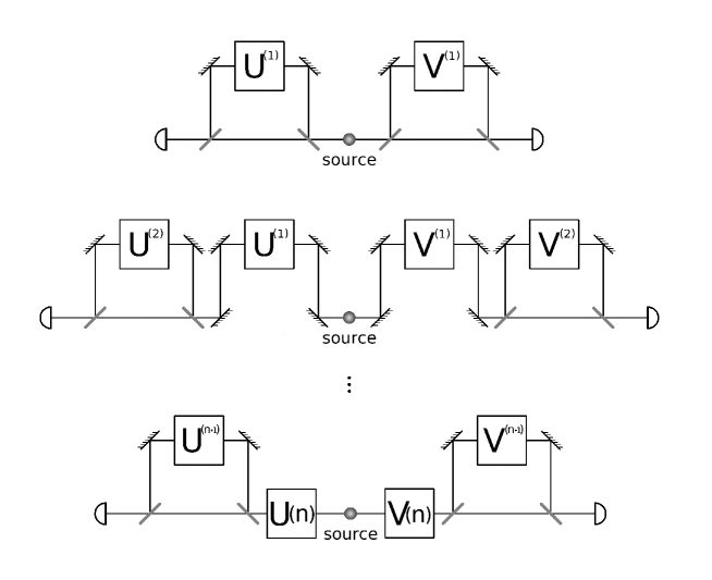
Figure 2: Iterative procedure in first, second and $(n+1)$th step.

The coincidence intensity in the $(n+1)$th step is now

$$I^{(n+1)}=\frac{1}{2}+\frac{1}{2}\mathrm{Re}\Tr\left[(\hat{U}^{(n+1)}\!\otimes\!\hat{V}^{(n+1)})({\hat{U}(n)\!\otimes\!\hat{V}(n)})\hat{\rho}^{(0)}({\hat{U}(n)^{\dagger}\!\otimes\!{\hat{V}(n)^{\dagger}}})\right],$$

where the cumulated unitary operations that are applied to the original input state $\hat{\rho}^{(0)}$ at the beginning of the $(n+1)$th step are $\hat{U}(n)\equiv{\hat{U}^{(n)}\hat{U}^{(n-1)}}\dots{\hat{U}^{(1)}}$ and $\hat{V}(n)\equiv{\hat{V}^{(n)}\hat{V}^{(n-1)}\dots{\hat{V}^{(1)}}}$.

From this we can define a holonomy group $Hol_{S}$ based on a particular state $\hat{\rho}_{0}$ with corresponding Stokes tensor $S$ as the set of unitary operators $\hat{V}(n)\equiv{\hat{V}^{(n)}\hat{V}^{(n-1)}\dots{\hat{V}^{(1)}}}\in{U(D_{B})}$ that can result from the above parallel transport prescription given all sequences of $\hat{U}^{(k)}\in{U(D_{A})}$ such that $\hat{U}(n)\equiv\hat{U}^{(n)}\hat{U}^{(n-1)}\dots{\hat{U}^{(1)}}=\hat{1}$ for any $n$. From the discussion on product states at the end of section 3.1 follows that the holonomy group for product states is always Abelian, and only correlated states can induce a non-Abelian holonomy group.

For any set of unitaries $\{\hat{U}^{(n)}\in{U}(D_{A})\}$ given by

$$\hat{U}^{(n)}=U^{(n)}_{0}\hat{1}^{A}+\sum_{k=1}^{D_{A}^{2}-1}U^{(n)}_{k}\hat{\chi}^{A}_{k},$$ (39)

we find $\hat{V}^{(n)}\in{U(D_{B})}$ that maximizes the intensity as

$$\hat{V}^{(n)}=\sum_{j,k=0}^{D_{B}^{2}-1}\sum_{l=0}^{D_{A}^{2}-1}B^{-1}_{jk}(\lambda^{(n)},\bar{\mu}^{(n)})S_{kl}^{T}U^{(n)*}_{l}\hat{\chi}^{B}_{j},$$

where $S_{lk}=\Tr\left[{(\hat{\chi}^{A}_{l}\!\otimes\!\hat{\chi}^{B}_{k})({\hat{U}(n-1)\!\otimes\!\hat{V}(n-1)})\hat{\rho}^{0}(\hat{U}(n-1)^{\dagger}\!\otimes\!\hat{V}(n-1)^{\dagger}})\right]$.

To define a connection we need to consider the limit when $\hat{U}$ and $\hat{V}$ are infinitesimally close to unity. To find this limit we revisit the maximization problem with a different parametrization $\hat{U}=e^{i\sum_{j=0}^{D_{A}^{2}-1}\theta_{j}\hat{\chi}_{j}^{A}}$ and $\hat{V}=e^{i\sum_{j=0}^{D_{B}^{2}-1}\phi_{j}\hat{\chi}^{B}_{j}}$. The intensity is then

$$I^{AB}={\frac{1}{2}+\frac{1}{2}\mathrm{Re}\Tr(e^{i\sum_{j=0}^{D_{A}^{2}-1}\!\!\theta_{j}\hat{\chi}_{j}^{A}}\otimes e^{i\sum_{j=0}^{D_{B}^{2}-1}\!\!\phi_{j}\hat{\chi}^{B}_{j}}\hat{\rho}_{0})},$$ (41)

where $\theta_{j}$ and $\phi_{j}$ are real numbers. In this representation unitarity is explicit and no constraints are necessary. Differentiating $I^{AB}$ with respect to the parameters $\phi_{j}$ and setting each derivative to zero, we find

$$\mathrm{Re}\Tr(e^{i\sum_{k=0}^{D_{A}^{2}-1}\!\!\theta_{k}\hat{\chi}^{A}_{k}}\otimes{i}\hat{\chi}^{B}_{j}{e}^{i\sum_{l=0}^{D_{B}^{2}-1}\!\!\phi_{l}\hat{\chi}^{B}_{l}}\hat{\rho}_{0})=0,\phantom{uuuuu}0\leq j\leq D_{B}^{2}-1.$$

Since we are only interested in finding the connection form we expand these equations to linear order in $\theta_{j}$ and $\phi_{j}$, to obtain

$$\mathrm{Re}\Tr\!\left[\!\left(\hat{1}^{A}\!+i\sum_{k=0}^{D_{A}^{2}-1}\!\theta_{k}\hat{\chi}^{A}_{k}\right)\!\!\otimes\!{i\hat{\chi}^{B}_{j}}\!\!\left(\hat{1}^{B}\!+i\!\!\sum_{l=0}^{D_{B}^{2}-1}\!\phi_{l}\hat{\chi}^{B}_{l}\right)\!\hat{\rho}_{0}\right]\!=$$

$$=\!\left(\!-\left\{\!\sum_{k=0}^{D_{B}^{2}-1}\!\!\phi_{k}S_{0k}\delta_{j0}+\phi_{0}S_{0j}\!+\!\left[\frac{2}{D_{B}}+\!\left(\!1-\frac{2}{D_{B}}\!\right)\!\!\delta_{j0}\right]\!\!\phi_{j}\!\right\}\!-\!\!\sum_{k,l=1}^{D_{B}^{2}-1}\!\!\phi_{k}d_{jkl}S_{0l}\right)$$

$$-\sum_{k=0}^{D_{A}^{2}-1}\theta_{k}S_{kj}=0,\phantom{uuuuuuuuuuu}0\leq j\leq D_{B}^{2}-1.$$ (43)

In the infinitesimal limit we introduce the notation $d\hat{U}\hat{U}^{\dagger}\equiv{i}(\sum_{j=0}^{D_{A}^{2}-1}d\theta_{j}\hat{\chi}^{A}_{j})$ and likewise $d\hat{V}\hat{V}^{\dagger}\equiv{i}(\sum_{j=0}^{D_{A}^{2}-1}d\phi_{j}\hat{\chi}^{A}_{j})$. Although performing infinitesimal unitary operations is clearly an idealization we may still consider this limit where the sequences of unitaries $\{\hat{\Delta}_{U}^{(t)}\equiv{\hat{1}^{A}+d\hat{U}\hat{U}^{\dagger}(t)}\}$ and $\{\hat{\Delta}_{V}^{(t)}\equiv{\hat{1}^{B}+d\hat{V}\hat{V}^{\dagger}(t)}\}$ in the parallel transport are indexed by a continuous variable $t$.

The relation between $\{\hat{\Delta}_{U}^{(t)}\}$ and $\{\hat{\Delta}_{V}^{(t)}\}$, for each $t$, is given by

$$\sum_{k=0}^{D_{B}^{2}-1}B_{jk}({dVV}^{\dagger})_{k}(t)=-\sum_{k=0}^{D_{A}^{2}-1}({dUU}^{\dagger})_{k}(t)S_{kj},$$ (44)

where $B_{jk}$ are the elements of the symmetric matrix $B$, given as

$$B_{jk} = \mathrm{Re}\Tr(\hat{\chi}^{B}_{j}\hat{\chi}^{B}_{k}\hat{\rho}^{B})=$$

$$= \left[\frac{2}{D_{B}}\delta_{kj}+\left(1-\frac{2}{D_{B}}\right)\delta_{j0}\delta_{k0}\right]+\sum_{l=1}^{D_{B}^{2}-1}S_{0l}\left[(\delta_{j0}\delta_{lk}+\delta_{k0}\delta_{lj})+d_{jkl}\right].$$

Therefore, provided $B$ is invertible, we find

$$\hat{\Delta}_{V}=\hat{1}^{B}-\sum_{k=0}^{D_{A}^{2}-1}\sum_{l,m=0}^{D_{B}^{2}-1}(dUU^{\dagger})_{k}S_{kl}{B}^{-1}_{ml}\hat{\chi}^{B}_{m}.$$ (46)

We can now identify

$$\hat{A}(t)\equiv-\sum_{k=0}^{D_{A}^{2}-1}\sum_{l,m=0}^{D_{B}^{2}-1}(dUU^{\dagger})_{k}S_{kl}{B}^{-1}_{ml}\hat{\chi}^{B}_{m}$$ (47)

as the operator-valued anti-Hermitean connection one-form. Note that $\hat{A}$ is a linear function of the Stokes matrix $S$. If we decompose the density operator as $\hat{\rho}=\sum_{\mu}p_{\mu}\mid\!\psi_{\mu}\rangle\langle\psi_{\mu}\!\mid$ we can express the connection form as

$$\hat{A}(t)=i\sum_{\mu}p_{\mu}\!\!\!\sum_{j,l=0}^{D_{B}^{2}-1}\!\!\mathrm{Re}\!\Tr(\hat{1}^{A}\!\otimes\!i\hat{\chi}^{B}_{j}\mid\!d{\psi}_{\mu}(t)\rangle\langle\psi_{\mu}(t)\!\mid)B^{-1}_{jl}\hat{\chi}^{B}_{l}.$$ (48)

Under a change of gauge $\mid\!{\psi}_{k}\rangle\to{\hat{1}^{A}\!\otimes\!\hat{G}}\!\mid\!{\psi}_{k}\rangle$, corresponding to a unitary transformation on the second subsystem, the connection transforms as

$$\hat{A}\!\to\!\!\hat{A}^{{}^{\prime}}\!\!=\!i\!\sum_{\mu}p_{\mu}\!\!\!\!\!\!\sum_{j,l,m,n=0}^{D_{B}^{2}-1}\!\!\!\!\!\!\mathrm{Re}\!\Tr[\hat{1}^{A}\!\!\otimes\!i\hat{\chi}^{B}_{j}\!\!\mid\!\!d(\hat{1}^{A}\!\!\otimes\!\hat{G}{\psi}_{\mu})\rangle\langle\psi_{\mu}\hat{1}^{A}\!\!\otimes\!\hat{G}^{\dagger}\!\!\mid]R_{jl}B^{-1}_{lm}R^{T}_{mn}\hat{\chi}^{B}_{n}\!\!=$$

$$=i\!\sum_{\mu}p_{\mu}\!\!\!\!\!\!\sum_{j,l,m,n=0}^{D_{B}^{2}-1}\!\!\!\!\!\!\mathrm{Re}\!\Tr[\hat{1}^{A}\!\otimes\!\hat{G}^{\dagger}i\hat{\chi}^{B}_{j}(\hat{G}\mid\!d{\psi}_{\mu}\rangle+d\hat{G}\mid\!{\psi}_{\mu}\rangle)\langle\psi_{\mu}\!\mid]R_{jl}B^{-1}_{lm}R^{T}_{mn}\hat{\chi}^{B}_{n}=$$

$$=i\!\sum_{\mu}p_{\mu}\!\!\!\!\!\!\sum_{h,j,l,m,n=0}^{D_{B}^{2}-1}\!\!\!\!\!\!\mathrm{Re}\!\Tr[\hat{1}^{A}\!\otimes\!i\hat{\chi}^{B}_{h}\mid\!{d\psi}_{\mu}\rangle\langle\psi_{\mu}\!\mid]R^{T}_{hj}R_{jl}B^{-1}_{lm}R^{T}_{mn}\hat{\chi}^{B}_{n}$$

$$+i\!\sum_{\mu}p_{\mu}\!\!\!\!\!\!\sum_{h,j,l,m,n=0}^{D_{B}^{2}-1}\!\!\!\!\!\!\mathrm{Re}\!\Tr[\hat{1}^{A}\!\otimes\!i\hat{\chi}^{B}_{h}\hat{G}^{\dagger}d\hat{G}\mid\!{\psi}_{\mu}\rangle\langle\psi_{\mu}\!\mid]R^{T}_{hj}R_{jl}B^{-1}_{lm}R^{T}_{mn}\hat{\chi}^{B}_{n}=$$

$$=\hat{G}d\hat{G}^{\dagger}+\hat{G}\hat{A}\hat{G}^{\dagger},$$ (49)

where $R_{jk}=\frac{1}{[\delta_{k0}(D_{B}-2)+2]}\Tr(\hat{G}\hat{\chi}_{k}^{B}\hat{G}^{\dagger}\hat{\chi}_{j}^{B})$, and we have used that $B_{jk}=\mathrm{Re}\Tr(\hat{\chi}^{B}_{j}\hat{\chi}^{B}_{k}\hat{\rho}^{B})$ which transforms as $B\to{RBR^{T}}$. Thus $\hat{A}$ transforms as a proper gauge potential.

For a given path $\gamma$ in $U(N_{A})$ given by $\hat{U}(t)$, the parallel transport gives us a path $\hat{V}(t)$ in $U(N_{B})$

$$\hat{V}(t)={\bf{P}}\!\left[\exp\left(\int_{0}^{t}\hat{A}(s)ds\right)\right],$$ (50)

where ${\bf{P}}$ denotes path ordering. The holonomy for a closed path in $U(N_{A})$ is thus given by such an integral and is dependent on the Stokes matrix via the connection form in equation (47).

5 Relation to Lévay parallel transport for $SU(2)\times{SU}(2)$

The pure two-qubit states can be represented as quaternionic qubit states [23, 24] using the structure of the second Hopf-fibration. Within this representation one can construct the quaternionic analogue of the Pancharatnam geometric phase, as has been done by Lévay [24]. We review this quaternionic representation and show that when the state evolution is generated by local $SU(2)$ operators, the Lévay geometric phase is contained in our construction.

In the quaternionic representation a pure two-qubit state

$$\mid\!{\psi}\rangle=\alpha\!\mid\!{00}\rangle+\beta\!\mid\!{01}\rangle+\gamma\!\mid\!{10}\rangle+\delta\!\mid\!{11}\rangle,$$ (51)

where $\alpha,\beta,\gamma,\delta\in{\mathbb{C}}$, is associated with a quaternionic qubit state

$$\mid\!\mathbf{\Psi}\rangle=(\alpha+\beta{\mathbf{j}})\mid\!\mathbf{0}\rangle+(\gamma+\delta{\mathbf{j}})\mid\!\mathbf{1}\rangle.$$ (52)

Here the quaternionic state $\mid\!\mathbf{0}$$\rangle$ is formed by identifying $\mid\!{00}\rangle$ and $\mid\!{01}\rangle$ in such a way that the complex coefficients of these states are contained in the new quaterionic coefficient, and similarly for $\mid\!\mathbf{1}$$\rangle$. The standard quaternion basis elements ${\mathbf{i}}$, ${\mathbf{j}}$ and ${\mathbf{k}}$, satisfy ${\mathbf{i}}^{2}={\mathbf{j}}^{2}={\mathbf{k}}^{2}=-1$ and ${\mathbf{i}}{\mathbf{j}}=-{\mathbf{j}}{\mathbf{i}}={\mathbf{k}}$. A local $SU(2)$ unitary $\hat{U}$ acting on the first qubit is represented by a operator $\hat{\bf{U}}$ acting from the left on $\mid\!\mathbf{\Psi}\rangle$ and a local $SU(2)$ unitary $\hat{V}$ acting on the second qubit is represented by a unit quaternion $q_{V}$ acting from the right

$$\mid\!\mathbf{\Psi}\rangle=\hat{{\bf{U}}}\mid\!\mathbf{\Psi_{0}}\rangle\hat{q}_{V},$$ (53)

where $\hat{{\bf{U}}}={U}_{0}\hat{{\bf{1}}}+i\sum_{j=1}^{3}{U}_{j}\hat{{\boldsymbol{\sigma}}}_{j}$ with $\hat{{\bf{1}}}$ and $\hat{\boldsymbol{\sigma}}_{1},\hat{\boldsymbol{\sigma}}_{2},\hat{\boldsymbol{\sigma}}_{3}$ the standard unit and Pauli operators acting on the quaternionic qubit Hilbert space. The unit quaternion $\hat{q}_{V}\in{Sp(1)}$ corresponds to $\hat{V}$ according to

$$\hat{V} = V_{0}\hat{1}^{B}+i\sum_{j=1}^{3}V_{j}\hat{\sigma}_{j}^{B}$$

$$\phantom{hjhjh}\updownarrow$$

$$\hat{q}_{V} = V_{0}+V_{3}\mathbf{i}-V_{2}\mathbf{j}+V_{1}\mathbf{k},$$ (54)

where $\hat{\sigma}_{1}^{B},\hat{\sigma}_{2}^{B},\hat{\sigma}_{3}^{B}$ are the standard Pauli operators acting on the state space of the second qubit.

The inner product of two quaternionic states $\mid\!\!\mathbf{\Psi}\rangle=p_{1}\!\mid\!\mathbf{0}\rangle+q_{1}\!\mid\!\mathbf{1}\rangle$ and $\mid\!\!\mathbf{\Phi}\rangle=p_{2}\!\mid\!\mathbf{0}\rangle+q_{2}\!\mid\!\mathbf{1}\rangle$ is

$$\langle\mathbf{\Psi}\!\mid\!\mathbf{\Phi}\rangle=q_{1}^{*}q_{2}+p_{1}^{*}p_{2},$$ (55)

where $*$ is the quaternionic conjugation operation defined by $(a+b\mathbf{i}+c\mathbf{j}+d\mathbf{k})^{\ast}=(a-b\mathbf{i}-c\mathbf{j}-d\mathbf{k})$, $a,b,c,d\in\mathbb{R}$.

The quaternionic transition amplitude between two states related by a local $SU(2)$ operation $\hat{U}$ on the first qubit can be expressed in terms of transition amplitudes in the ordinary complex representation as

$$\langle\mathbf{\Psi}\!\mid\hat{{\bf{U}}}\mid\!\mathbf{\Psi}\rangle=U_{0}+\sum_{j=1}^{3}U_{j}M_{j3}\mathbf{i}-\sum_{j=1}^{3}U_{j}M_{j2}\mathbf{j}+\sum_{j=1}^{3}U_{j}M_{j1}\mathbf{k},$$ (56)

where $\mid\!\!\psi\rangle$ and $\mid\!\!\mathbf{\Psi}\rangle$ are the complex and quaternionic representations of the same state. From this we can consider the formal analogue of the Mach-Zehnder interference intensity

$$I = \frac{1}{2}+\frac{1}{2}\mathrm{Re}(\langle\mathbf{\Psi}\!\mid\hat{{\bf{U}}}\mid\!\mathbf{\Psi}\rangle\hat{q}_{V})$$ (57)

$$= \frac{1}{2}+\frac{1}{2}U_{0}V_{0}-\frac{1}{2}\!\!\sum_{j,k=1}^{3}\!\!\!U_{j}V_{k}M_{jk},$$

where the phase factor $\hat{q}_{V}$ represents a local $SU(2)$ operation on the second qubit. To compare this intensity to the Franson interference intensity for the case $\hat{U}\in{SU(2)}$ and $\hat{V}\in{SU(2)}$, we consider equation (32) when $D_{A}=2$ and use the parameterization $\hat{U}=U_{0}\hat{1}^{A}+i\sum_{j=1}^{3}U_{j}\hat{\sigma}_{j}^{A}$, where $U_{0},U_{1},U_{2},U_{3}$ are real numbers. We then find that the quaternionic Mach-Zehnder interference intensity $I$, is identical to the Franson intensity $I^{AB}$, which demonstrates the correspondence between the quantum-mechanical Franson setup and the quaternionic quantum-mechanics Mach-Zehnder setup as shown in figure 3.

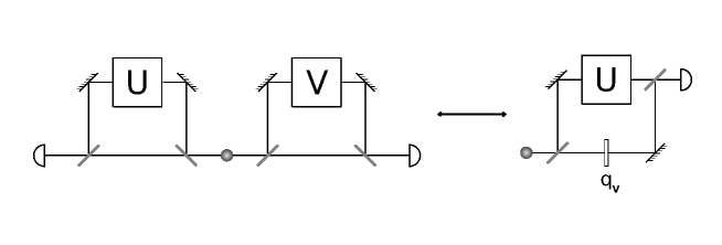
Figure 3: Correspondence between Franson setup and quaternionic QM Mach-Zehnder setup

This quaternionic representation of the two-qubit states can be considered a generalization of the ordinary complex spinor representation of single qubits. In the ordinary single qubit representation, the Hilbert space is the space of normalized complex spinors $S^{3}$ and the projective Hilbert space is the space of spinors modulo a phase factor $S^{3}/U(1)={S}^{3}/S^{1}=S^{2}=\mathbb{C}P^{1}$, the complex projective space of complex dimension one. In this quaternionic representation of two-qubit states, the Hilbert space is the space of normalized quaternionic spinors $S^{7}$. The quaternionic projective Hilbert space is the space of quaternionic spinors modulo a unit quaternion acting from the left, representing, as mentioned above, a $SU(2)={S}^{3}$ rotation of the second qubit. This implies that the quaternionic projective Hilbert space is $S^{7}/S^{3}=S^{4}=\mathbb{H}P^{1}$, the quaternionic projective space of quaternionic dimension one, or real dimension $4$. While the ordinary single qubit representation corresponds to the first Hopf fibration $S^{1}\hookrightarrow{S}^{3}\hookrightarrow{S}^{2}$, the quaternionic two qubit representation corresponds to the second Hopf fibration $S^{3}\hookrightarrow{S}^{7}\hookrightarrow{S}^{4}$. This quaternionic two-qubit representation is much similar to a qubit in quaternionic quantum mechanics [31] except that in this representation the absolute quaternionic phase corresponds to a rotation of the second qubit and thus is a measurable quantity.

Within this representation of pure two qubit states, Lévay [24] studied the quaternionic analogue of the Pancharatnam parallel transport. Lévay’s parallelity condition and related parallel transport are defined such that two quaternionic states are parallel if their inner product is a real and positive number. This condition is in concordance with the Mach-Zehnder analogue picture since the maximal intensity is achieved when the unit quaternion phase factor $\hat{q}_{V}$ is such that $\langle\mathbf{\Psi}\!\mid\!\hat{U}\!\mid\!\mathbf{\Psi}\rangle\hat{q}_{V}$ is real and positive. We next consider a family of spinors that are stepwise unitarily evolved from the same initial state $\mid\!\mathbf{\Psi}_{0}\rangle$ and demand that in each step the initial and final states are parallel. The transition amplitude between two consecutive spinors in this family is

$$\langle\mathbf{\Psi}_{n-1}\!\mid\!\mathbf{\Psi}_{n}\rangle=\langle\mathbf{\Psi}_{n-1}\!\mid\hat{{\bf{U}}}^{(n)}\mid\!\mathbf{\Psi}_{n-1}\rangle\hat{q}_{V}^{(n)}=\lambda,\phantom{hhhhhh}\lambda\in{\mathbb{R}_{+}},\!\!\!\!\!\!$$

where $\mid\!\mathbf{\Psi}_{n-1}\rangle=\!\hat{{\bf{U}}}\!(n-1)\mid\!\mathbf{\Psi}_{0}\rangle{\hat{q}_{V}}(n-1)$, and we use the notation $\hat{{\bf{U}}}(n-1)=\hat{{\bf{U}}}^{(n-1)}\hat{{\bf{U}}}^{(n-2)}\dots{\hat{{\bf{U}}}^{(1)}}$ and $\hat{q}_{V}(n-1)=\hat{q}_{V}^{(1)}\hat{q}_{V}^{(2)}\dots{\hat{q}_{V}^{(n-1)}}$. Thus

$$\langle\mathbf{\Psi}_{n-1}\!\mid\hat{{\bf{U}}}^{(n)}\mid\!\mathbf{\Psi}_{n-1}\rangle=\lambda{q}_{V}^{(n)\ast},$$ (59)

or by using equations (5) and (56)

$$U^{(n)}_{0}\! + \!\sum_{j=1}^{3}\!U^{(n)}_{j}\!M_{j3}\mathbf{i}-\!\!\sum_{j=1}^{3}\!U^{(n)}_{j}\!M_{j2}\mathbf{j}+\!\!\sum_{j=1}^{3}\!U^{(n)}_{j}\!M_{j1}\mathbf{k}=$$ (60)

$$= \lambda(V^{(n)}_{0}-V^{(n)}_{3}\mathbf{i}+V^{(n)}_{2}\mathbf{j}-V^{(n)}_{1}\mathbf{k}).$$

Hence

$$V^{(n)}_{0} = \frac{1}{\lambda}U^{(n)}_{0},$$

$$V^{(n)}_{j} = -\frac{1}{\lambda}\sum_{k=1}^{3}U^{(n)}_{k}M_{kj}.$$ (61)

The parameter $\lambda$ must be chosen to normalize $V^{(n)}$, hence $\lambda^{2}=U^{(n)2}_{0}+\sum_{i}(\sum_{j}U^{(n)}_{j}M_{ji})^{2}$. If we compare this to equation (33), when $D_{A}=2$ and again use the parameterization $\hat{U}=U_{0}\hat{1}^{A}+i\sum_{j=1}^{3}U_{j}\hat{\sigma}_{j}^{A}$, where $U_{0},U_{1},U_{2},U_{3}$ are real numbers, we find that this parallelity condition is the same as that in equation (61).

To find the Lévay connection, we consider the infinitesimal limit in which the parallel transport condition reads

$$\langle{d}\mathbf{\Psi}\!\mid\!\mathbf{\Psi}\rangle=0,$$ (62)

where $\mid\!\mathbf{\Psi}\rangle$ is the instantaneous state. If we only allow changes generated by the local unitaries $\hat{{\bf U}}$ and $q_{V}$ we have

$$\langle{d}\mathbf{\Psi}\!\mid{\mathbf{\Psi}}\rangle=d{q_{V}}^{\ast}q_{V}+\langle d\mathbf{\Psi}\!\mid{\hat{{\bf U}}}d{\hat{{\bf U}}}^{\dagger}\mid{\mathbf{\Psi}}\rangle.$$ (63)

Imposing the parallel transport condition $\langle{d}\mathbf{\Psi}\!\mid\!{\mathbf{\Psi}}\rangle=0$, and using equations (5) and (56) we find this to be equivalent to

$$(dVV^{\dagger})_{j}=-\sum_{k=1}^{3}(dUU^{\dagger})_{k}M_{kj}.$$ (64)

To compare this expression with the connection in our construction we consider equation (44) for $D_{A}=D_{B}=2$, and note that for $SU(2)$ all symmetric structure constants $d_{jkl}$ are zero. This gives the $B$ matrix the following form

$$B=\left(\begin{array}[]{cccc}1&S_{01}&S_{02}&S_{03}\\ S_{10}&1&0&0\\ S_{20}&0&1&0\\ S_{30}&0&0&1\end{array}\right).$$ (69)

By taking into account that $(dUU^{\dagger})_{0}=0$ and $(dVV^{\dagger})_{0}=0$ for $SU(2)$, we see that only the correlation matrix $M$ will be relevant to the relation between $\hat{dUU}^{\dagger}$ and $\hat{dVV}^{\dagger}$. Since $B_{jk}=\delta_{jk}$ for $j,k\neq 0$ it immediately follows that equation (44) reduces to equation (64).

6 Conclusion

We have constructed a parallel transport procedure in the same spirit as that of Pancharatnam [6, 7, 8], in the sense that it defines parallelity with reference to maximization of an interferometric quantity. The interferometric quantity chosen in this case is the coincidence intensity of a Franson type interferometer. The phase is taken to be the local degrees of freedom of one of the subsystems.

Given two different two-partite states related by local unitary evolution of one of the subsystems, the unitary operation that needs to be applied to the other subsystem to achieve parallelity, depends on the correlation present in the full bipartite system. Generally phase unitaries that correspond to different parallel transports do not commute, however, when the system is uncorrelated, only Abelian phase factors need to be applied. Thus the holonomy group related to the parallel transport condition is Abelian if the bipartite state is uncorrelated, and a non-Abelian holonomy group can be said to be correlation induced.

The procedure is defined for arbitrary bipartite systems, pure as well as mixed. In the infintesimal limit of the parallel transport, the connection form can be found as a closed expression for arbitrary dimension. On the other hand, finding a closed expression for parallel transport when the steps are finite appears to be non-trivial in the general $U(D)$ case. The procedure can be restricted to subgroups of the full unitary groups. In the pure two-qubit case when only $SU(2)$ operators are considered it has been shown that this procedure is related to Lévay parallel transport [24]. Therefore our construction opens up for experimental tests of the Lévay geometric phase in the special case of local $SU(2)$ evolutions.

References

- [1] Berry M V 1984 Proc. Roy. Soc. London A 392 45
- [2] Aharanov Y and Anandan J 1987 Phys. Rev. Lett. 58 1593
- [3] Wilzcek F and Zee A 1984 Phys. Rev. Lett. 52 2111
- [4] Anandan J 1988 Phys. Letters A 133 171
- [5] Sjöqvist E, Pati A K, Ekert A, Anandan J S, Ericsson M, Oi D K L and Vedral V 2000 Phys. Rev. Lett. 85 2845
- [6] Pancharatnam S 1956 Proc. Ind. Acad. Sci. A 44 247
- [7] Berry M V 1987 J. Mod. Opt. 34 1401
- [8] Ramaseshan S and Nityananda R 1986 Curr. Sci. 55 1225
- [9] Mead C A 1991 Phys. Rev. A 44 1473
- [10] Anandan J and Pines A 1989 Phys. Lett. A 141 335
- [11] Kult D, Åberg J and Sjöqvist E 2006 Phys. Rev. A 74 022106
- [12] Sjöqvist E, Kult D and Åberg J 2006 Phys. Rev. A 74 062101
- [13] Williamson M S and Vedral V 2009 Open. Syst. Info. Dyn. 26 305
- [14] Williamson M S and Vedral V 2007 Phys. Rev. A 76 032115
- [15] Williamson M S 2009 Ph.D. Thesis, University of Leeds
- [16] Wootters W K 2002 J. Math. Phys. 43 4307
- [17] Wagh A G and Rakhecha V C 1995 Phys. Lett. A 197 107
- [18] Wagh A G, Rakhecha V C, Fisher P and Ioffe A 1998 Phys. Rev. Lett. 81 1992
- [19] Horne M A, Shimony A and Zeilinger A 1989 Phys. Rev. Lett. 62 2209
- [20] Franson J D 1989 Phys. Rev. Lett. 62 2205
- [21] Franson J D 1991 Phys. Rev. A 44 4552
- [22] Hessmo B and Sjöqvist E 2000 Phys. Rev. A 62 062301
- [23] Mosseri R and Dandoloff R 2001 J. Phys. A: Math. Gen. 34 10243
- [24] Lévay P 2004 J. Phys. A: Math. Gen. 37 1821
- [25] Jaeger G 2007 Quantum Information: An Overview (Boston MA: Springer)
- [26] Horodecki R and Horodecki M 1996 Phys. Rev. A 54 1838
- [27] Ericsson Å 2002 Phys. Lett. A 295 256
- [28] Wootters W K 1998 Phys. Rev. Lett. 80 2245
- [29] Werner R F 1989 Phys. Rev. A 40 4277
- [30] Caves C M, Fuchs C A and Rungta P 2001 Found. Phys. Lett. 14 199
- [31] Adler S and Anandan J 1996 Found. Phys. 26 1579