Manifold learning techniques and model reduction applied to dissipative PDEs

Abstract

We link nonlinear manifold learning techniques for data analysis/compression with model reduction techniques for evolution equations with time scale separation. In particular, we demonstrate a “nonlinear extension” of the POD-Galerkin approach to obtaining reduced dynamic models of dissipative evolution equations. The approach is illustrated through a reaction-diffusion PDE, and the performance of different simulators on the full and the reduced models is compared. We also discuss the relation of this nonlinear extension with the so-called nonlinear Galerkin methods developed in the context of Approximate Inertial Manifolds.

1 Introduction

The purpose of this paper is to extend established model reduction methods for large-scale dynamical systems characterized by separation of time scales by linking them to recently developed (nonlinear) manifold learning techniques–in particular, with the diffusion map (DMAP) approach of Coifman and coworkers [5, 6]; see also [1].

The general setting involves a high-dimensional, stiff system of differential equations of the form

$$\frac{d\vec{y}}{dt}=\vec{f}(\vec{y})$$ (1)

with $\vec{f}:\,\,\mathbf{R}^{d}\longrightarrow\mathbf{R}^{d}$. We will focus on problems where this system arises in the context of discretizing a dissipative partial differential equation: an equation of the form

$$\frac{\partial}{\partial t}u+Au=F(u),$$ (2)

where $A$ is a positive self-adjoint operator with a discrete spectrum and $F(u)$ is a “well-behaved” function of $u$ [8, 9, 15, 35, 18, 46]. We chose this type of example because we will later draw some analogies between our approach and the so-called nonlinear Galerkin reduction techniques [16, 14, 26, 18, 46] developed in precisely this context of Approximate Inertial Manifolds. We note, however, that the reduction procedure we will discuss can also be attempted for large systems of ODEs characterized by separation of time scales (and the associated stiffness) that arise in other situations–for example, in large, complicated chemical kinetic networks.

For our prototypical system (equation (1)), there exists a slow, attracting, invariant manifold to which trajectories quickly decay. In the framework of Approximate Inertial Manifolds, this means that when solutions to equation (2) are projected onto the complete set of eigenfunctions of $A$, the long-term behavior of the solution components in the higher eigenfunctions can be parameterized by (depicted as a graph of a function over) the solution components in the leading eigenfunctions. The result is a low-dimensional manifold in an infinite-dimensional space (or, for truncated approximations, in a high-dimensional space). Given a collection of points sampled from such a manifold, we wish to develop a reduced set of dynamic equations that describe the dynamics on this manifold. Ideally, the dimensionality of this reduced set would be the “intrinsic” dimension of the long-term dynamics: the dimension of the manifold. Nonlinear Galerkin techniques share this goal, but they are not based on data sampling on the manifold; they are based instead on approximating it as a graph of a function above the first few eigenfunctions of the operator (or eigenvectors in the case of its discretization). What we propose here is an extension of what is referred to as “the POD-Galerkin approach”–sampling data on the manifold, using Principal Component Analysis (PCA) to compress the data (see, e.g. [24]), and performing (various forms of) Galerkin projection of the dynamics on the leading POD modes to obtain reduced models of the long-term dynamics themselves (see, e.g., [23, 12, 30, 3, 44]). Since principal component analysis passes optimal (in a well-defined sense) approximating hyperplanes through the data points, one can easily envision intrinsically low-dimensional (but curved) manifolds that require much higher dimensional hyperplanes to successfully embed them. Remedying this potential discrepancy between intrinsic manifold dimension and the lowest-dimensional POD-Galerkin that can successfully reproduce the long-term dynamics is the focus of this work.

Modern manifold learning techniques can be thought of as (nonlinear) extensions of PCA, in the sense that they “learn” the geometry of the low-dimensional manifolds on which the data lie, and pass optimal (again in a well-defined sense) nonlinear approximating manifolds through the data points. Our procedure utilizes diffusion maps (DMAPs) to learn the geometry of the slow manifold from simulation data, and the related Nyström extension to rewrite the dynamics of (1) exploiting this geometry. Some interpolation (in the form of the Nyström extension) is required, but it is performed in the reduced-dimension embedding space (as opposed to the original, high-dimensional, data space). Model dimensionality as well as model equation stiffness is thus hopefully reduced, so that both explicit and implicit temporal integration methods may exhibit savings over the original, full model simulation. The premise is that the “basis functions” provided by the DMAP process can be (sometimes significantly) fewer in number than the basis functions provided by methods such as POD, since they represent the true underlying dimensionality of the slow manifold.

Reducing the model with the help of these “nonlinear” modes can help identify significant components of the dynamics, enhance intuition about the dynamical system behavior, and faciliate computations. We will see, however, that the nonlinearity of the reduction technique also gives rise to certain difficulties, which may offset the benefit of the “more parsimonious” manifold parametrization. Other approaches to model reduction can be analytical, such as “quasi-steady-state”/partial-equilibrium assumptions [39, 41], or computer-assisted, such as the rate-controlled constrained equilibrium method (RCCE) [27], computational singular perturbation (CSP) [32], intrinsic low-dimensional manifolds (ILDM) [34] (essentially, first-order CSP), functional iteration [40], and even conditions on various derivatives [19, 20, 10, 29, 33, 47].

The paper is organized as follows. We start with a concise description of DMAPs for manifold learning using high-dimensional data. We then briefly review the POD-Galerkin approach, and present our method as its natural nonlinear analogue. We then compare our method with nonlinear Galerkin reduction techniques through an illustrative example, and conclude with a brief summary and discussion of open problems and possible extensions.

2 Brief introduction to DMAPs

Diffusion maps have recently emerged as a fast, robust, nonlinear dimensionality reduction tool [5, 6]; see also [1]. Starting with an ensemble of data (e.g. points in a high-dimensional space), diffusion maps (DMAPs) help determine whether they can be embedded in a lower-dimensional space, and also find and parametrize a “best” (and possibly nonlinear) low-dimensional manifold that (approximately) contains the data. In actuality, the only input to the DMAP algorithm is a scalar similarity measure between each pair of entries in the data ensemble; therefore, DMAPs can also be used on data that are not necessarily points in Euclidean space [11, 13, 45]. In our context, however, the data ensemble does consist of points (represented as vectors) sampled from ODE trajectories; we therefore present the DMAP algorithm for data ensembles that consist of vectors $\vec{X}_{i}\in\mathbf{R}^{d}$. Typically, the similarity measure becomes negligible beyond a local neighborhood of each data point; this is related to the notion that large Euclidean distances may not reliably approximate geodesic distances on a general nonlinear manifold. These pairwise similarities are used in the DMAP algorithm to construct a matrix whose leading eigenvectors nonlinearly embed the data set in a lower-dimensional Euclidean space. Euclidean distance in the new, reduced space approximates the diffusion distance, a quantity related to manifold geodesic distance (for a rigorous definition of the diffusion distance see [7]). The DMAP can thus provide a global manifold parametrization based on local information only, much like the unfolding of a crumpled towel to a two-dimensional rectangle.

To construct a low-dimensional embedding for a data set of $M$ individual points (represented as $d$-dimensional real vectors, $\vec{X}_{1}$,…,$\vec{X}_{M}$) we start with a similarity measure between each pair of vectors $\vec{X}_{i}$, $\vec{X}_{j}$. The similarity measure is a nonnegative quantity $W(i,j)=W(j,i)$ satisfying certain additional “admissibility conditions” [5]. As a concrete example, consider the Gaussian and Epanechnikov similarity measures (based on the standard $L^{2}$ norm):

$$W(i,j)=\text{exp}\left[-\left(\frac{\left\|\vec{X}_{i}-\vec{X}_{j}\right\|}{\epsilon}\right)^{2}\right]$$ (3)

and

$$W(i,j)=(1-\left\|\vec{X}_{i}-\vec{X}_{j}\right\|^{2}/\epsilon^{2})\mathbf{1}_{\{\left\|\vec{X}_{i}-\vec{X}_{j}\right\|<\epsilon\}}.$$ (4)

A weighted Euclidean norm may be chosen over the standard $L^{2}$ norm in situations where the values of different components of $\vec{X}$ may vary over disparate orders of magnitude. $\epsilon$ defines a characteristic scale which quantifies the “locality” of the neighborhood within which Euclidean distance can be used as the basis of a meaningful similarity measure [5]. A systematic approach to determining appropriate $\epsilon$ values is discussed below.

Next, we define the diagonal matrix $\mathbf{D}$ by

$$D(i,i)=\sum^{M}_{k=1}W(i,k),$$

and then we compute the first few right eigenvectors corresponding to the largest eigenvalues of the stochastic matrix

$$\mathbf{K}=\mathbf{D}^{-1}\mathbf{W}.$$

In MATLAB, for instance, this can be done with the command $[\mathbf{V},\mathbf{L}]=\mbox{eigs}(\mathbf{K},n)$, where $n$ is the number of top eigenvalues we wish to keep (we typically are only interested in the first few).

This gives a set of real eigenvalues $\lambda_{0}\geq\lambda_{1}\geq...\geq\lambda_{n}\geq...\geq 0$ with corresponding eigenvectors $\{\vec{\psi}_{j}\}_{j=0}^{n}$. Since $\mathbf{K}$ is stochastic, $\lambda_{0}=1$ and $\vec{\psi}_{0}=[1\,1\,...\,1]^{T}$. The $n$-dimensional representation of a particular $d$-dimensional data vector, $\vec{X}_{i}$, is given by the diffusion map $\vec{\Psi}_{n}:\,\mathbf{R}^{d}\longrightarrow\mathbf{R}^{n}$, where

$$\vec{\Psi}_{n}(\vec{X}_{i})=[\lambda_{1}^{t}\vec{\psi}_{1}^{(i)},\lambda_{2}^{t}\vec{\psi}_{2}^{(i)},...,\lambda_{n}^{t}\vec{\psi}_{n}^{(i)}],$$

a mapping which is only defined on the $M$ recorded data vectors. Here, $t$ represents the “diffusion time”; to keep things simple, we choose $t=1$. In other words, the vector $\vec{X}_{i}$ is mapped to a vector whose first component is the $i$th component of the first nontrivial eigenvector, whose second component is the $i$th component of the second nontrivial eigenvector, etc. If a gap in the eigenvalue spectrum is observed between eigenvalues $\lambda_{n}$ and $\lambda_{n+1}$, then $\vec{\Psi}_{n}$ may provide a useful low-dimensional representation of the data set [1, 36]. In fact, when this gap is present (and when the DMAP is scaled as $\vec{\Psi}_{n}(\vec{X}_{i})=[\lambda_{1}\vec{\psi}_{1}^{(i)},\lambda_{2}\vec{\psi}_{2}^{(i)},...,\lambda_{n}\vec{\psi}_{n}^{(i)}]$), Euclidean distance in the DMAP space of only these first $n$ eigenvectors will accurately approximate the diffusion distance mentioned above.

We choose the value of $\epsilon$ used in the DMAP computation by invoking the correlation dimension [22]. The assumption here is that the volume of an $n$-dimensional set scales with any characteristic length $s$ as $s^{n}$; for relatively uniform sampling one might expect the number of neighbors less than $s$ apart to scale similarly. We demonstrate this technique on a simple illustrative data set (points sampled from a one-dimensional curve, see Figure 1 below) by first computing all pairwise Euclidean distances. Figure 1 shows $L(\epsilon)$, the total number of pairwise distances less than $\epsilon$; it is clear that an asymptote will arise at large $\epsilon$ ($M^{2}$, where $M$ is the number of points) and at small $\epsilon$ ($M$). In the figure, the two asymptotes are smoothly connected by an approximately straight line; the slope of this line suggests the correct dimensionality for our data set (here, one). The range of $\epsilon$ values corresponding to this straight segment are all acceptable in our DMAP computations: here any value of $\epsilon$ between approximately $10^{-2}$ and $10^{0}$ may be used. Figure 1 also schematically illustrates the difference between PCA-based and DMAP-based reduction; the data are in the form of a two-dimensional spiral embedded in three-dimensional space. Using the original coordinates to parametrize this spiral requires three coordinates, while using PCA requires two and DMAPs require only one (since the actual dimensionality of the spiral is one).

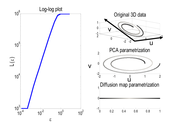
Fig. 1: Left: log-log plot of $L(\epsilon)$, a statistic of the data set (see text) vs. $\epsilon$. For $M$ data vectors, $\lim_{\epsilon\to\infty}L(\epsilon)$ is simply $M^{2}$ and $\lim_{\epsilon\to 0}L(\epsilon)$ is simply $M$. These two asymptotes are connected, however, by an approximately straight line. $\epsilon$ values chosen from this regime are appropriate for our DMAP calculations. Right: three parametrizations of the same two-dimensional spiral embedded in three-dimensional space (again, see text).

3 Ambient space to DMAP space and back

In order to utilize the model reduction machinery provided by diffusion maps, one must be able to map back and forth between the original, high-dimensional ambient space and the reduced, low-dimensional DMAP space. From the original space to DMAP space, there exists a mathematically elegant approach known as Nyström extension; the reverse map, however, is more difficult.

3.1 Nyström extension

The problem of finding the DMAP coordinates of a new $d$-dimensional vector $\vec{X}_{\mbox{new}}$ (a point not contained in the original data set) is solved with the Nyström extension. The first step is to compute all distances $\{d_{i\,\text{new}}\}_{i=1}^{M}$ (or at least those which do not give a negligible similarity measure) between our new vector and the $M$ vectors in our data set, and set, for instance $W(i,\text{new})=W(\text{new},i)=\text{exp}\left[-\left(\frac{d_{i\,{\text{new}}}}{\epsilon}\right)^{2}\right]$ or $W(i,\text{new})=W(\text{new},i)=(1-d_{i\,{\text{new}}}^{2}/\epsilon^{2})\mathbf{1}_{\{d_{i\,{\text{new}}}<\epsilon\}}$ (corresponding to equations (3) and (4), respectively). Setting

$$K(i,\text{new})=\left(\sum_{k=1}^{M}W(k,\text{new})\right)^{-1}W(i,\text{new}),$$

the $j\text{th}$ DMAP coordinate (there are $n$ coordinates total) of the new vector $\vec{X}_{\mbox{new}}$ is given by

$$\vec{\psi}_{j}(\vec{X}_{\mbox{new}})=\frac{1}{\lambda_{j}}\sum_{i=1}^{M}K(i,\text{new})\,\vec{\psi}_{j}^{(i)}.$$

We typically drop the $n$ from $\vec{\Psi}_{n}$ (again, $n$ denotes the number of DMAP coordinates we choose to retain, and thus, the dimension of our DMAP space), and denote this process of Nyström extension as $\vec{\Psi}(\vec{X})$. Clearly, this extension procedure will return a result even if $\vec{X}_{\mbox{new}}$ is not chosen to be exactly on our low-dimensional manifold

3.2 Construction of an “inverse Nyström map”

An important component of our reduced computations below is the ability to transform from DMAP space back to ambient space. In other words, for given values of low-dimensional DMAP coordinates, we wish to find the corresponding “on manifold” point in the high-dimensional Euclidean space where the original data ensemble lies. Approaches proposed include simulated annealing [13], Newton iteration, polynomial interpolation, interpolation using radial basis functions [38], manifold regularization [2], and geometric harmonics [4]. The method we chose here is polynomial interpolation of the ambient coordinates over DMAP space; each coordinate of ambient space is written as a polynomial over the low-dimensional DMAP space. Polynomial interpolation is used simply because it is easy to derive order of magnitude error estimates; yet one should mention (even though this was not observed in our computations) that singular matrices can, in principle, arise in the process (see, e.g. the discussion in [38]) The geometric harmonics extension scheme, akin to Fourier interpolation on manifolds, may very well outperform polynomial interpolation and is described below.

Since this transformation process is analogous to an approximate inverse of the diffusion map (we go from low-dimensional DMAP space to high-dimensional ambient space), we denote it as $\vec{\Psi}_{n}^{-1}(\vec{L})$, or simply $\vec{\Psi}^{-1}(\vec{L})$, for $\vec{L}\in\mathbf{R}^{n}$ (DMAP space).

3.2.1 Polynomial interpolation

Suppose we wish to find $\vec{X}\in\mathbf{R}^{d}$ on the manifold such that for a given $\vec{L}\in\mathbf{R}^{n}$,

$$\vec{L}=\vec{\Psi}_{n}(\vec{X})\mbox{, or, as we indicated above, simply }\vec{L}=\vec{\Psi}(\vec{X}).$$

We first determine the $K$ closest points to $\vec{L}$ in our data set (with proximity measured in DMAP space) and note both the DMAP coordinates $\{\vec{L}_{l}\}_{l=1}^{K}$ and corresponding ambient space coordinates $\{\vec{X}_{l}\}_{l=1}^{K}\in\mathbf{R}^{d}$ of these $K$ points. These points are used to compute the coefficients of a local polynomial interpolation of each ambient space coordinate over the DMAP coordinates; for each coordinate $j=1,2,...,d$ of ambient space, we determine the coefficients for the polynomial interpolation using $\{\vec{L}_{1},\vec{X}_{1}^{(j)}\},\{\vec{L}_{2},\vec{X}_{2}^{(j)}\},...,\{\vec{L}_{K},\vec{X}_{K}^{(j)}\}$, and we denote the result as $P^{(j)}$, setting $\vec{X}^{(j)}=P^{(j)}(\vec{L})$. This procedure is relatively fast because the polynomials are constructed over $\mathbf{R}^{n}$, and $n$ has been assumed small. For example, in the reaction-diffusion example that follows, we choose $K=10$ and interpolate over the two-dimensional DMAP space using six overall (up to quadratic) terms. The six coefficients are fitted through least squares since, for $K=10$, the system is overdetermined (only $K=6$ is required). The result of this procedure is a point $\vec{\Psi}^{-1}(\vec{L})$ which is an approximation of the corresponding “true,” on-manifold point. The error introduced by this approximation will affect our reduced dynamical model computations, as we will mention below.

3.2.2 Geometric harmonics

An additional computational tool from harmonic analysis which can be used for interpolation and extrapolation is geometric harmonics [4, 31]. We do not use this tool here, since it is difficult for us to derive order-of-error bounds; we do, however, feel that it is an important option, and -while we omit many significant mathematical details- we include here a brief description, for completeness. The geometric harmonics extension scheme, inspired by the Nyström extension scheme, is a method for extending functions defined over some smaller set $X$ to a larger one $\bar{X}$ [4]. This is exactly the problem of constructing the inverse Nyström map; for each point in our data ensemble, we know both its DMAP coordinates and its ambient space coordinates (this can be viewed as $d$ functions from DMAP space ($\mathbf{R}^{n}$) to each coordinate in ambient space), and we now wish to know this function for new values of the DMAP coordinates as well. Throughout, we use $f$ to denote the function we desire to extend from $X$ to $\bar{X}$.

We first choose a symmetric, positive semi-definite kernel $k:\,\bar{X}\times\bar{X}\rightarrow\mathbf{R}$ such as $k(x,y)=\mbox{exp}\left(-\left\|x-y\right\|^{2}/\epsilon^{2}\right)$. Here, $\epsilon$ quantifies the distance away from the data set $X$ that we wish to be able to extend our function $f(\bar{X})$. The key observation is that when $f$ oscillates with frequency $\nu$, it cannot be extended reliably beyond a distance of $O(1/\nu)$. This makes intuitive sense, as interpolation of functions $f$ which change rapidly should not be trusted far from the “known” values of $f$. For demonstration, a geometric harmonics extension of the function $f(\theta)=\cos(2\theta)$ is shown in Figure 2, where $\theta=\mbox{arctan}\frac{y}{x}$ and the set $X$ is simply the circle in $\mathbf{R}^{2}$ given by $x^{2}+y^{2}=1$. For $\epsilon=0.5$, the extension of $f$ onto the plane is “wider” (see Figure 2) than for the case $\epsilon=0.1$, but as we will see, this comes with the trade-off of increased extension error (here, the error is measured on the “known” set $X$, see below). Here, it is worth noting that, due to the nature of the kernel $k$ used, this formulation bears a strong resemblance to function approximation procedures using radial basis functions (RBFs) (see, e.g. [17]).

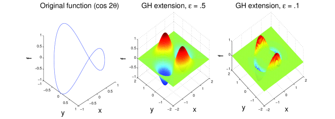
Fig. 2: The original function of $f=\cos(2\theta)$, defined on the unit circle (left), is extended with $\epsilon=0.5$ (middle) and $\epsilon=0.1$ (right).

We can restrict this kernel to $X$ and define the linear operator $\mathbf{K}$ as

$$\mathbf{K}f(\bar{x})=\int_{X}k(\bar{x},x)f(x)d\mu(x),$$

where $\mu(x)$ is just the measure of the set $X$ (if the data set consists of $M$ random samples, $\mu(x)=1/M$ is typically used). It can be shown that this operator has a discrete set of eigenvalues $\{\lambda_{j}\}\geq 0$ (in nonincreasing order) and orthonormal eigenfunctions $\{\tau_{j}\}$ so that for almost all $x\in X$,

$$\lambda_{j}\tau_{j}(x)=\int_{X}k(x,y)\tau_{j}(y)d\mu(y).$$

Over finite sets, these integrals are obviously just sums and the eigenfunctions are just eigenvectors. The geometric harmonics are defined as the extension of the eigenfunctions to $\bar{X}$ via

$$\tau_{j}(\bar{x})=\frac{1}{\lambda_{j}}\int_{X}k(\bar{x},y)\tau_{j}(y)d\mu(y)$$

for $\lambda_{j}\neq 0$. Since $\lambda_{j}\rightarrow 0$ as $j\rightarrow\infty$, this extension procedure becomes numerically ill-conditioned. We pick a condition number $1/\delta$, and let $S_{\delta}=\{j\mbox{ such that }\lambda_{j}\geq\delta\lambda_{0}\}$. We can now extend $f(X)$ to $f(\bar{X})$ as follows:

1. Project $f$ onto the numerically acceptable eigenfunctions via

   $$f(x)\rightarrow\sum_{j\in S_{\delta}}\langle f,\tau_{j}\rangle_{X}\tau_{j}(x),\quad\mbox{where $\langle\,\rangle$ denotes inner product}.$$ (5)

2. Use $\tau_{j}$ to extend $f$ on $\bar{X}$ as

   $$f(\bar{x})=\sum_{j\in S_{\delta}}\langle f,\tau_{j}\rangle_{X}\tau_{j}(\bar{x}).$$

With a fine kernel (small $\epsilon$) there is negligible error in the projection of $f$ in equation (5) (here, the error is measured on the “known” set $X$); the eigenvalues decay slowly enough so that most of the eigenfunctions can be used ($\lambda_{j}\geq\delta\lambda_{0}$ for most $j$). However, $\tau_{j}(\bar{x})$ quickly decays to zero for any $\bar{x}$ much farther away from the data set $X$ than $\epsilon$ because there, the kernel function $k$ practically vanishes. With a coarser kernel (large $\epsilon$), there may be more error in the projection projection of $f$ in equation (5) (again measured on the “known” set $X$) since most eigenfunctions are neglected. However, the domain of extendability is much larger. Because of this, a multiscale extension scheme is usually used in practice. In such a scheme, $f$ is first projected at a coarse scale (large $\epsilon$), and then the error in this initial coarse projection (the residual $f$) is projected at a finer scale (smaller $\epsilon$). The error in this second, finer projection is then projected at an even finer scale, and this process is continued until the total error shrinks below some desired threshold. The sum of these projections yields the extended $f$ function. Often, an initial $\epsilon=\epsilon_{0}$ is chosen, and then during projection $i$, $\epsilon=2^{-(i-1)}\epsilon_{0}$ [4]. $f$ is therefore extended as a linear combination of functions which oscillate with frequency $\nu_{j}$ and which vanish at a distance $O(1/\nu_{j})$ from the set $X$. Several results about the mathematical optimality of the extension of $f$ by this procedure have been obtained [4].

4 Dynamics in reduced spaces

As we outlined in the introduction, we begin with the setting of a dissipative partial differential equation of the form

$$\frac{\partial}{\partial t}u+Au=F(u),$$

operating on a function $u(\vec{x},t)$. The usual stipulation is for $F$ to be globally Lipshitz continuous and at least $C^{1}$, while $A$ is a self-adjoint, compact linear operator; slightly different requirements are possible (see, e.g., [16, 14, 26, 18, 46]). After a Galerkin projection of this equation using the eigenfunctions of $A$, one obtains a stiff system of ODEs which describes the evolution of the coefficients of the projection of the solution (projections onto these eigenfunctions of $A$). Although the spectrum of $A$ is typically countably infinite, one often truncates the eigenfunction expansion with only $d$ eigenfunctions, where $d$ is chosen based on some physical intuition or specified error. Under appropriate conditions, one can also obtain a low-dimensional manifold of dimension $n<d$ in phase space to which trajectories are quickly attracted, due to the dissipative nature of the PDE [16, 14, 26, 18, 46].

To illustrate the application of model reduction to dissipative PDEs, we utilize the Chafee-Infante reaction-diffusion equation

$$u_{t}-\nu u_{xx}+u^{3}-u=0,$$ (6)

with $\nu=0.16$ and periodic boundary conditions $u(0,t)=u(\pi,t)=0$. This equation is exactly of the form of equation (2) with $Au=\nu u_{xx}$ and $F(u)=u-u^{3}$, and it is known to have a two-dimensional inertial manifold [25].

We first perform a Galerkin projection of this equation onto the first $d=10$ Fourier modes ($\sin x$, $\sin 2x$, $\ldots$, $\sin 10x$), resulting in an equation of the form of (1):

$$\frac{d\vec{y}}{dt}=\vec{f}(\vec{y}),$$

where $\vec{y}\in\mathbf{R}^{10}$ denotes the vector of coefficients of the Galerkin projection, $u(x,t)=\sum_{i=1}^{10}\vec{y}^{(i)}(t)\sin ix$. In the literature, the $i$th Fourier mode is usually denoted as $a_{i}$ instead of $\vec{y}^{(i)}$; this will be the convention we adopt when referring to the Fourier modes of the reaction-diffusion equation. Next, we obtain a data set $\vec{X}_{1},\vec{X}_{2},...,\vec{X}_{M}\in\mathbf{R}^{10}$ sampled from the two-dimensional, slow, inertial manifold by randomly generating initial conditions and integrating these initial conditions for a brief ($t=1$) amount of time (sufficient enough for a decay to the slow manifold). Finally, we use these vectors $\vec{X}_{1},\vec{X}_{2},\ldots,\vec{X}_{M}$ in order to perform the model reduction outlined in §4.1 and 4.2 below.

4.1 Proper orthogonal decomposition

Discretely sampling simulation trajectories after the initial (brief) approach to the attracting manifold will give rise to an ensemble of data points that have been computed and saved as vectors in $\mathbf{R}^{d}$. We can attempt to compress these data by taking advantage of the low dimensionality of the manifold that they live on; this is traditionally accomplished through the use of Principal Component Analysis (PCA) on the data. If we find that most of the energy (defined in terms of vector inner products in $\mathbf{R}^{d}$) of the data can be spanned by the first $n$ eigenvectors of the PCA decomposition, this suggests that the data can be efficiently described as vectors in $\mathbf{R}^{n}$ (as the components of the data in the directions of the first $n$ eigenvectors). PCA, in addition to simple data compression, can also form the basis of a systematic way to

1. reduce the dynamics of the original high-dimensional (here, $d$-dimensional) dynamical system to $k$ dimensions

2. rewrite the correponding dynamics in the new, reduced, low-dimensional space

using again a Galerkin procedure. One starts with the data set $\vec{X}_{1},\vec{X}_{2},...,\vec{X}_{M}\in\mathbf{R}^{d}$ sampled from the (long term dynamics on the) low-dimensional, slow, invariant, attracting manifold. These $\vec{X}$ may come from a variety of sources. Here, we have chosen to focus on $\vec{X}$ which represent the coefficients of the spectral representation of solutions of equation (2), but these $\vec{X}$ may also be the concentrations of various chemical species for the slow manifold of a chemical kinetics problem.

POD finds (for each $n=1,2,...,d$) the projection onto the $n$th dimensional linear subspace which maximizes the variance of the projected data. Let us denote the projection of a vector in $\vec{X}\in\mathbf{R}^{d}$ onto this linear subspace as $\mathbf{P}_{n}(\vec{X})$. Defining $\vec{c}^{(l)}=\frac{1}{M}\sum_{k=1}^{M}\vec{X}_{k}^{(l)}$, $\mathbf{P}_{n}(\vec{X})$ can be written as $\mathbf{P}_{n}(\vec{X})=\vec{c}+\sum_{k=1}^{n}\langle\vec{X}-\vec{c},\vec{p}_{k}\rangle\vec{p}_{k}$. Here, we have $\langle\vec{p}_{k},\vec{p}_{j}\rangle=\delta_{kj}$, and the $\{\vec{p}_{k}\}_{k=1}^{d}$ are the eigenvectors of the matrix $\mathbf{\tilde{X}}\mathbf{\tilde{X}}^{T}$ with

$$\mathbf{\tilde{X}}=\left[\begin{array}[]{cccc}|&|&&|\\ \vec{X}_{1}-\vec{c}&\vec{X}_{2}-\vec{c}&...&\vec{X}_{M}-\vec{c}\\ |&|&&|\end{array}\right].$$

It turns out that regardless of the final dimension $n$ of the linear subspace, the first projection direction remains optimal, as does the second, third, etc.; these $\{\vec{p}_{k}\}_{k=1}^{n}$ do not change with $n$. Defining $\vec{L}\in\mathbf{R}^{n}$ as the coefficients of the projection in this reduced space, $\vec{L}^{(1)}=\langle\vec{X}-\vec{c},\vec{p}_{1}\rangle$, $\vec{L}^{(2)}=\langle\vec{X}-\vec{c},\vec{p}_{2}\rangle$, etc., we write $\vec{L}=\vec{P}_{n}(\vec{X})$. The Galerkin reformulation then yields the reduced dynamics of the $\vec{y}$ of equation (1) in this $n$-dimensional space. If $\vec{L}=\vec{P}_{n}(\vec{y})$, then:

$$\frac{d\vec{L}}{dt} = \frac{d}{dt}\vec{P}_{n}(\vec{y})$$

$$= \vec{P}_{n}\left(\frac{d}{dt}\vec{y}\right)$$

because $\vec{P}_{n}$ is linear. Continuing,

$$\frac{d\vec{L}}{dt} = \vec{P}_{n}\left(\vec{f}(\vec{y})\right)$$

$$\approx \vec{P}_{n}\left(\vec{f}\left(\vec{c}+\sum_{k=1}^{n}\vec{L}^{(k)}\vec{p}_{k}\right)\right)$$

so that now things are expressed in terms of $\vec{L}$. Evaluating the right hand side is a challenge often requiring quadrature or involving cumbersome analytical formulas (unless $f$ is linear).

When the slow manifold of the system is not a linear subspace, this method will not give much information about the underlying dimensionality of the slow manifold because the number of modes used is often based on some sort of error control and not on manifold geometry. It will also take more modes (larger $n$) than the dimensionality of the slow manifold to accurately represent the dynamics. Figure 3 illustrates this by showing a one-dimensional (nonlinear) curve lying in three-dimensional space, respresentative of the possibility of one-dimensional dynamics in a higher-dimensional space. Figure 4 shows, in terms of a Fourier basis for the solution (again, denoted $a_{1},a_{2},\ldots$) of the reaction-diffusion equation (6), two slices of the two-dimensional (but nonlinear) inertial manifold of the (high-dimensional) reaction-diffusion equation; again, the long-term dynamics are low-dimensional while the ambient space dimension is high. In these situations, a technique is desired in which we may write the reduced dynamics of equation (1) on the actual, low-dimensional slow manifold regardless of its shape or of whether it can be approximated by a hyperplane.

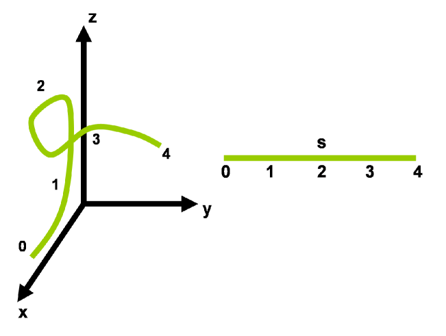
Fig. 3: A one-dimensional curve, representing a one-dimensional slow manifold in three-dimensional space, is shown (left). The curve is not a straight line, and it requires three POD modes to be well represented. Ideally, we would like to write the slow dynamics in terms of one “mode;” for example, $(x(s),y(s),z(s))$ as a function of arclength $s$ (right). Such a parametrization can be found using DMAPs.

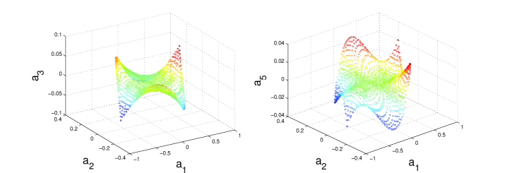
Fig. 4: For a particular class of reaction-diffusion equations and for certain parameter values, an inertial manifold of dimension $2$ exists [25], parametrized in Fourier space by the first two Fourier modes $(a_{1},a_{2})$. For visualization purposes, we have shown two “slices” of this inertial manifold, $a_{3}(a_{1},a_{2})$ and $a_{5}(a_{1},a_{2})$, in three-dimensions (with points colored by $a_{3}$ and $a_{5}$, respectively). It is clear that both of these slices are highly nonplanar and that any sort of two-dimensional POD plane would do a poor job passing through or near all these points.

4.2 The DMAP approach

In contrast to POD, whose model reduction is based upon the discovery of a linear subspace which approximately contains the slow manifold, diffusion maps allow us to write the dynamics of equation (1) on the “true” low-dimensional (and possibly nonlinear) slow, attractive, invariant manifold.

In this section, we use DMAPs to find a parametrization of the slow manifold and denote the dimensionality reduction procedure as $\vec{L}=\vec{\Psi}_{n}(\vec{X})$, or, as before, we drop the $n$ and write $\vec{L}=\vec{\Psi}(\vec{X})$, where $\vec{L}\in\mathbf{R}^{n}$. Here, $\Psi$ is a transformation from the high-dimensional ambient space to the low-dimensional parametrization. In our working example, the Chafee-Infante reaction-diffusion equation (6), the inertial manifold is two-dimensional; we therefore expect $\vec{\Psi}_{2}$ to give us our manifold parametrization. In Figure 4, we show a picture of the two-dimensional reaction-diffusion inertial manifold in only three-dimensional ambient space for visualization purposes.

We now derive the reduced dynamics of equation (1). If $\vec{L}=\vec{\Psi}(\vec{y})$ (and $\vec{y}=\vec{\Psi}^{-1}(\vec{L})$), then:

$$\frac{d\vec{L}}{dt} = \frac{d}{dt}\vec{\Psi}(\vec{y})$$

$$= \frac{\partial\,\vec{\Psi}(\vec{y})}{\partial\vec{y}}\,\frac{d\vec{y}}{dt}$$

by the chain rule, where $\frac{\partial\,\vec{\Psi}(\vec{y})}{\partial\vec{y}}$ is a $n\times d$ matrix and $\frac{d\vec{y}}{dt}$ is a $d$-dimensional vector. Continuing,

$$\frac{d\vec{L}}{dt} = \frac{\partial\,\vec{\Psi}(\vec{y})}{\partial\vec{y}}\,\vec{f}(\vec{y})$$ (7)

$$= \frac{\partial\,\vec{\Psi}\left(\vec{\Psi}^{-1}\left(\vec{L}\right)\right)}{\partial\vec{y}}\,\vec{f}\left(\vec{\Psi}^{-1}\left(\vec{L}\right)\right)$$

so that now things are expressed in terms of $\vec{L}$. Ways to obtain $\Psi^{-1}\left(\vec{L}\right)$ were discussed above (we used polynomial interpolation). It is worth noting again that Nyström extension, $\vec{\Psi}(\vec{y})$, will also return values for points $\vec{y}\in\mathbf{R}^{d}$ which are neither exactly on our manifold nor in the original data ensemble.

When new points $\vec{X}_{\mbox{new}}$ (points not in our original data ensemble) such as $\vec{\Psi}^{-1}(\vec{L})$ arise in the computation, we obtain $\frac{\partial\,\vec{\Psi}}{\partial\vec{y}}$ at such points as follows:

$$\vec{\Psi}^{(j)}(\vec{X}_{\mbox{new}}) = \frac{1}{\lambda_{j}}\sum_{i=1}^{M}K(i,\text{new})\,\vec{\psi}_{j}^{(i)}$$

$$= \frac{1}{\lambda_{j}}\frac{\sum_{i=1}^{M}W(i,\text{new})\,\vec{\psi}_{j}^{(i)}}{\sum_{i=1}^{M}W(i,\text{new})}.$$

Therefore,

$$\frac{\partial\vec{\Psi}^{(j)}}{\partial\vec{X}_{\mbox{new}}^{(k)}} = \frac{1}{\lambda_{j}}\,\frac{\partial}{\partial\vec{X}_{\mbox{new}}^{(k)}}\,\left(\frac{\sum_{i=1}^{M}W(i,\text{new})\,\vec{\psi}_{j}^{(i)}}{\sum_{i=1}^{M}W(i,\text{new})}\right)$$ (8)

$$= \frac{1}{\lambda_{j}}\frac{\sum_{l,i=1}^{M}\,W(l,\text{new})\left(\frac{\partial}{\partial\vec{X}_{\mbox{new}}^{(k)}}W(i,\text{new})\right)\left(\vec{\Psi}_{j}^{(i)}-\vec{\Psi}_{j}^{(l)}\right)}{\left(\sum_{i=1}^{M}W(i,\text{new})\right)^{2}}.$$

It is really only necessary to compute $W(i,\text{new})$ for those $\vec{X}$ which lie near $\vec{X}_{\mbox{new}}$ since for distances beyond $\epsilon$, contributions from other points either dies off (Gaussian kernel) or disappears completely (Epanechnikov kernel).

Now that we have these formulas, we can compute the dynamics of equation (7) starting from an initial condition in DMAP space. Even if this initial condition is selected to be one of the known data points, immediately after the first integration step, we will find the trajectory visiting “new” points $\vec{X}_{\mbox{new}}$ that do not belong to our original data set. When such new points arise, we are able to compute the necessary time derivatives via equation (8). Armed with these formulas, we can now continue the integration of equation (7), constantly going back and forth between DMAP and ambient representations in order to obtain the time derivatives in DMAP space.

To validate our approach, we compare two finite trajectories:

1. a trajectory begun at $\vec{X}(0)\in\mathbf{R}^{d}$, integrated according to equation (1) for time $t$

2. a trajectory begun at $\vec{\Psi}(\vec{X}(0))\in\mathbf{R}^{n}$ (DMAP space), integrated according to equation (7) for time $t$, and transformed back into the original, ambient space of $\mathbf{R}^{d}$ using $\vec{\Psi}^{-1}$.

We integrated these two trajectories very accurately using ode113 and absolute and relative error tolerances of 1e-7. A particular slice of these two $10$-dimensional trajectories is shown in Figure 5; clearly, they visually coincide (and do so for all other slices as well).

It is also interesting to observe that reduction in the number of variables also reduces the model problem’s stiffness. Numerically, we observe that for any $d$, the magnitude of the largest absolute eigenvalue of the Jacobian of the reformulated system (7) for our problem is $O(1)$, whereas the magnitude of the maximum absolute eigenvalue of the Jacobian of the original system (1) is $O(d^{2})$. The reason is that derivatives of $\vec{\Psi}(\vec{X})$ are zero in directions orthogonal to the slow manifold, so stiff directions (which in this example are approximately orthogonal to the manifold) are effectively projected out of equation (7). In fact, for certain error tolerances, computing the trajectories shown in Figure 5 using our approach takes less wall clock time than computing the trajectories via the original dynamics (1). With absolute and relative error tolerances of $10^{-6}$, for instance, ode45 spends $2.11$ seconds of wall clock time to compute the “new” dynamics, while the original dynamics takes $5.73$ seconds and three times as many calls to the derivative function. Explicit integrators are less susceptible to stability constraints due to the reduced stiffness (allowing fewer time steps), while implicit integrators fare well for an entirely different reason: the reduced dimensionality of the problem makes the computational linear algebra (in the Newton iterations required to solve the corresponding nonlinear equations of the implicit integrator) faster. Our purpose in this paper is to implement and discuss the procedures necessary for the formulation and solution of the reduced equations (7); a more quantitative comparison of the cost of integration of equations (1) and (7) is the subject of current research.

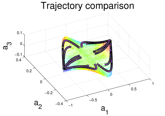
Fig. 5: A visual comparison of the trajectories obtained through the original dynamics of equation (1) (black) and the new dynamics of equation (7) (purple), shown for visualization purposes in three-dimensional space (points are colored by their value of $a_{3}$). To perform this comparison, the trajectory corresponding to the reformulated dynamics had to be transformed into the original space using the $\vec{\Psi}^{-1}(\vec{L})$.

There are two reasonable ways of quantifying the difference between the two sets of dynamics, the original dynamics (1) and the “new” dynamics of our approach (7). The first is to compare, in ambient space, the trajectories computed by our approach with those computed according to the original dynamics as in Figure 5. The second is to compare these two trajectories in DMAP space instead. Comparing trajectories in either DMAP space or ambient space requires first obtaining these trajectories, and thus making choices about the particular integrators; however, even when the two sets of equations (the original and the new) are integrated with great numerical accuracy, independent of cost, their trajectories will differ because of the interpolation (the $\vec{\Psi}^{-1}$ map) in equation (7). Furthermore, the original dynamics have a different dimensionality and stiffness than the dynamics of our approach. We therefore choose to focus on only the error involved in the evaluation of the right hand side of equation (7), the error in the DMAP-based dynamics.

Suppose the integrator (in DMAP space) produces a new point $\vec{L}$ (in DMAP space). The derivative at $\vec{L}$ constructued by equation (7) is only approximate because the $\vec{\Psi}^{-1}$ map is not exact (and this equation uses the $\vec{\Psi}^{-1}$ map twice). We use $\Delta\vec{x}$ to denote the $\vec{\Psi}^{-1}$ interpolation error:

$$\vec{\Psi}^{-1}\left(\vec{L}\right)=\vec{\Psi}^{-1}_{\mathbf{true}}\left(\vec{L}\right)+\Delta\vec{x}.$$

Now, we wish to study the error in equation (7) due to $\Delta\vec{x}$. Restricing our attention to a single coordinate $g\in 1,2,...,n$ of DMAP space, equation (7) takes the following form:

$$\frac{d\vec{L}^{(g)}}{dt} = \frac{\partial\,\vec{\Psi}^{(g)}\left(\vec{\Psi}^{-1}\left(\vec{L}\right)\right)}{\partial\vec{y}}\,\vec{f}\left(\vec{\Psi}^{-1}\left(\vec{L}\right)\right)$$ (9)

$$= \frac{\partial\,\vec{\Psi}^{(g)}\left(\vec{\Psi}_{\mathbf{true}}^{-1}\left(\vec{L}\right)+\Delta\vec{x}\right)}{\partial\vec{y}}\,\vec{f}\left(\vec{\Psi}_{\mathbf{true}}^{-1}\left(\vec{L}\right)+\Delta\vec{x}\right),$$

where, now, $\frac{\partial\,\vec{\Psi}^{(g)}}{\partial\vec{y}}$ is a $1\times d$ matrix. Expanding equation (9), and keeping only first order terms, we see that the error in coordinate $g$ is given as:

$$\mbox{err}^{(g)} \equiv \frac{d\vec{L}^{(g)}}{dt}-\frac{\partial\,\vec{\Psi}^{(g)}\left(\vec{\Psi}_{\mathbf{true}}^{-1}\left(\vec{L}\right)\right)}{\partial\vec{y}}\,\vec{f}\left(\vec{\Psi}_{\mathbf{true}}^{-1}\left(\vec{L}\right)\right)$$

$$\approx \Delta\vec{x}^{T}\,\,\frac{\partial^{2}\,\vec{\Psi}^{(g)}\left(\vec{\Psi}_{\mathbf{true}}^{-1}\left(\vec{L}\right)\right)}{\partial\vec{y}^{2}}\vec{f}\left(\vec{\Psi}_{\mathbf{true}}^{-1}\left(\vec{L}\right)\right)$$

$$\quad+\frac{\partial\,\vec{\Psi}^{(g)}}{\partial\vec{y}}\left(\vec{\Psi}_{\mathbf{true}}^{-1}\left(\vec{L}\right)\right)\mathbf{J}\left(\vec{\Psi}_{\mathbf{true}}^{-1}\left(\vec{L}\right)\right)\Delta\vec{x},$$

where $\frac{\partial^{2}\,\vec{\Psi}^{(g)}}{\partial\vec{y}^{2}}$ and $\mathbf{J}$ are $d\times d$ matrices (and $\mathbf{J}$ is the Jacobian of the function $\vec{f}$). Combining these terms, we see that the overall error in the $g$th component is bounded by

$$\left|\mbox{err}^{(g)}\right|\leq\left|\left|\Delta\vec{x}\right|\right|\left(\left|\left|\frac{\partial^{2}\,\vec{\Psi}^{(g)}}{\partial\vec{y}^{2}}\right|\right|\left|\left|\vec{f}\,\right|\right|+\left|\left|\frac{\partial\vec{\Psi}^{(g)}}{\partial\vec{y}}\mathbf{J}\right|\right|\right),$$

where $\|\,\,\|$ represents the matrix (vector) norm. Here, $\left\|\vec{f}\,\right\|$ should be small since it is evaluated “on manifold” at point $\vec{\Psi}_{\mathbf{true}}^{-1}\left(\vec{L}\right)$; essentially, since we are on the slow manifold, only slow derivatives are present. $\left\|\frac{\partial^{2}\,\vec{\Psi}^{(g)}}{\partial\vec{y}^{2}}\right\|$ can be shown to be bounded and $O(1)$ under appropriate scaling [31]. Finally, when the fast directions (eigenvectors of $\mathbf{J}$ with large negative eigenvalues) are approximately orthogonal to the manifold, as they are in our reaction-diffusion illustrative example, the norm of the $n\times d$ matrix $\frac{\partial\,\vec{\Psi}}{\partial\vec{y}}\mathbf{J}$ will be small (on the order of the eigenvalues of the slow subspace); the kernel of $\frac{\partial\,\vec{\Psi}}{\partial\vec{y}}$ consists of the directions orthogonal to the manifold.

4.3 Nonlinear Galerkin techniques

An alternative approach to obtaining accurate reduced discretizations of dissipative PDEs is provided by the so-called “nonlinear Galerkin” techniques in the context of approximate inertial manifolds. Instead of a Galerkin projection onto a large number of orthogonal eigenfunctions, leading to a large set of coupled ODEs, one (approximately) expresses the component of the solution in the “higher” modes as a function of its components in the “lower” modes (see, e.g., [8, 9, 15, 16, 14, 26, 35, 18, 46]).

For the two-dimensional reaction-diffusion inertial manifold above, for instance, it is known that one can approximate the coefficients of each of the higher-order Fourier modes ($a_{3},a_{4},a_{5},...$) on the slow manifold as functions of just the first two Fourier modes, $a_{1}$ and $a_{2}$. The nonlinear Galerkin formulation will then depend on only two variables, the first two Fourier modes, and the reduced dynamics are two-dimensional. Two popular techniques to approximate the slaving of the higher to the lower-order modes include the so-called “steady” and the “Euler-Galerkin” approximate intertial manifolds (AIMs).

The steady approximation for our reaction-diffusion problem is implemented by setting $\dot{a}_{3}=0$, $\dot{a}_{4}=0$, $\dot{a}_{5}=0$, …, from which we obtain the functions $a_{3}(a_{1},a_{2})$, $a_{4}(a_{1},a_{2})$, $a_{5}(a_{1},a_{2})$, … We evolved the steady approximate inertial form using MATLAB’s built-in Differential Algebraic Equation (DAE) solver ode15s. At 3.44 seconds, this code took longer than both the original and the DMAP-based dynamics; this may very well be because, even though the system is conceptually two-dimensional, the linear algebra computations in the DAE solver are performed in a higher (here, $10$) dimensional space.

In the Euler-Galerkin approximation the functions $\{a_{k}(a_{1},a_{2})\}_{k}$ are obtained by constraining $a_{1}$ and $a_{2}$ to be constant, and taking an implicit Euler step (for appropriately chosen size $\tau$) of the constrained dynamics of the higher-order Fourier modes. Here, as in [14], we used $\tau=1$, which is large enough for the higher-order modes to get slaved to the first two modes. Instead of solving the nonlinear equations resulting from the implicit Euler step, a fixed point iteration is implemented (and in fact, only a single substitution is performed, since the map is so contracting). For simplicity, we consider only $a_{1},a_{2},$ and $a_{3}$ and set $a_{4}=a_{5}=\cdots=0$. Then the constrained $a_{3}$ dynamics are given by

$$\dot{a}_{3} \equiv \dot{a}_{3\,\mbox{diffusive}}+\dot{a}_{3\,\mbox{reactive}}$$

$$= (-9\nu a_{3})+(a_{3}-3a_{3}^{3}-6a_{2}^{2}a_{3}-6a_{1}^{2}a_{3}+a_{1}^{3}-3a_{1}a_{2}^{2}).$$

Taking one implicit Euler step of length $\tau$ while holding $a_{1}$ and $a_{2}$ constant, and using as initial condition $a_{3}(0)=0$ ($0$ is a good initial guess since higher-order modes quickly become small), we obtain

$$a_{3}(\tau) = a_{3}(0)+\tau\dot{a}_{3}(\tau)$$

$$= 0+\tau\left[\dot{a}_{3\,\mbox{diffusive}}(a_{1},a_{2},a_{3}(\tau))+\dot{a}_{3\,\mbox{reactive}}(a_{1},a_{2},a_{3}(\tau))\right].$$

Moving the diffusive term to the left hand side,

$$(1+9\tau\nu)a_{3}(\tau)=\tau[a_{3}(\tau)-3a_{3}^{3}(\tau)-6a_{2}^{2}a_{3}(\tau)-6a_{1}^{2}a_{3}(\tau)+a_{1}^{3}-3a_{1}a_{2}^{2}].$$ (11)

The map $a_{3}\leftarrow\frac{\tau}{1+9\tau\nu}(a_{3}-3a_{3}^{3}-6a_{2}^{2}a_{3}-6a_{1}^{2}a_{3}+a_{1}^{3}-3a_{1}a_{2}^{2})$ can be shown to be a contraction, intuitively because of the large eigenvalues associated with the diffusion term. Hence, instead of solving equation (11), we invoke the method of successive substitutions with initial guess $a_{3}=0$ to obtain the approximation $a_{3}=\frac{\tau}{1+9\tau\nu}(a_{1}^{3}-3a_{1}a_{2}^{2})$.

A comparison of the exact manifold (from accurate full simulations), the steady AIM, and the Euler-Galerkin AIM can be seen in Figure 6. In Figure 7, we show the magnitude of the error (the norm of the vector

$$\left[(a_{3\,\mbox{computed}}-a_{3\,\mbox{exact}})\quad(a_{4\,\mbox{computed}}-a_{4\,\mbox{exact}})\quad...\quad\right]$$

of errors) for the manifold constructed by our inverse Nyström map (essentially a polynomial interpolation of points on the exact manifold), the steady AIM, and the Euler-Galerkin AIM.

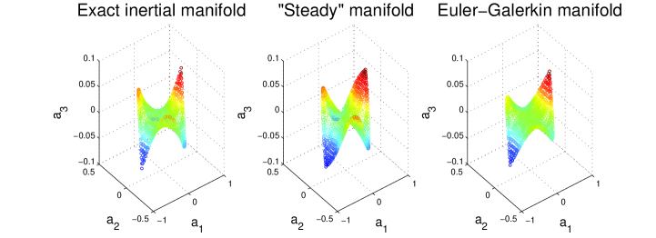
Fig. 6: A comparison of the exact inertial manifold with the two nonlinear Galerkin AIMs described in §4.3 (see text).

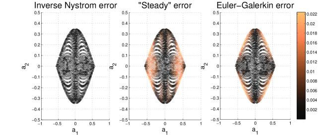
Fig. 7: A comparison of the errors of our inverse Nyström manifold (the “interpolated manifold” used to evolve equation (7)), the steady AIM, and the Euler-Galerkin AIM (see text).

We verified numerically that an isomorphism exists between the first two DMAP coordinates and the first two Fourier modes for points on the inertial manifold. This was established by verifying that the determinant of the Jacobian of the transformation from two-dimensional DMAP space to $(a_{1},a_{2})$ Fourier space is everywhere nonzero. This nonsingularity of the Jacobian is also suggested by Figure 8. As expected, the DMAP correctly captures the two-dimensional geometry of the slow manifold; the DMAP eigenvalues we computed for the data using $\epsilon=0.2$ are $(1.0,0.8477,0.7504,0.4585,0.4155,...)$, and the first two nontrivial eigenvalues are clearly larger than the rest.

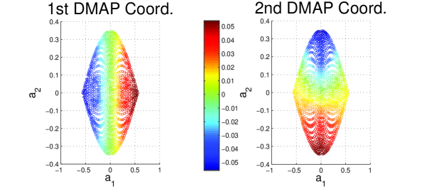
Fig. 8: A plot of the first DMAP coordinate (left) and the second DMAP coordinate (right) vs. the first two Fourier modes ($a_{1}$ and $a_{2}$). The figure strongly suggests that the determinant of the Jacobian is everywhere nonzero, or equivalently, that the transformation between the first two DMAP coordinates and the first two Fourier modes is unique; on the left, $a_{1}$ appears to be one-to-one with the first DMAP coordinate, and on the right, once a value of $a_{1}$ (equivalently, the first DMAP coordinate) is specified, $a_{2}$ one-to-one with the second DMAP coordinate.

5 Conclusion

In this paper we demonstrated a link between manifold learning techniques (and, in particular, diffusion maps) and model reduction for dissipative evolutionary PDEs. The approach is data-based, and it provides an interesting (“nonlinear”) alternative to the the well-known Galerkin projection of the dynamics on the leading principal components of the data ensemble. The implementation of the algorithm is only slightly more involved than that of the classic POD-Galerkin method, and is often faster due to decreased stiffness and a more parsimonious dimensionality reduction; the latter case occuring with low-dimensional but highly nonlinear (non-flat) slow manifolds residing in high-dimensional ambient spaces.

Instead of evaluating $d\vec{L}/dt$ from the right hand side of equation (7), it is also possible to perform a short integration in physical space, transform the resulting trajectory into DMAP space, and use the transformed trajectory to estimate $d\vec{L}/dt$ “on demand.” This is reminiscent of the “Galerkin-free” computations of [43], where this approach was exploited to avoid the construction of the right-hand-side of a POD-Galerkin dynamical system. In that case, short bursts of physical simulation observed in POD space were used to estimate the time-derivatives of the POD components of the solution; these provided the input to projective integrators (see, e.g., [28, 21]).

Having extrapolated the POD component values to future times, it is easy to construct physical initial conditions consistent with these values. In our case, however, having extrapolated the DMAP solution coordinates to future times, it is more difficult to find off-sample physical initial conditions consistent with these extrapolated values; our inverse Nyström map ($\vec{\Psi}^{-1}$) relied on polynomial interpolation.

Our work started with an available ensemble of points on the manifold, without any sense of the trajectories from which these points were sampled; if we have the trajectories themselves, as well as time-derivatives (evaluated or estimated) at every sample point, then adaptive tabulation tools (see, e.g., [37]) can again help circumvent the cumbersome computation of the right-hand-side of equation (7).

We believe that manifold-learning techniques of the type we discussed here, and the reduced models they lead to, may be particularly useful for tasks for which small dimensionality is crucial (such as the approximation of stable manifolds or visualization of the dynamics).

6 Acknowledgments

I. G. K. and A. S. are pleased to acknowledge motivating discussions with Dr. R. Erban and Prof. M. S. Jolly.

References

- [1] M. Belkin and P. Niyogi, Laplacian eigenmaps for dimensionality reduction and data representation, Neural computation, 15 (2003), pp. 1373–1396.
- [2] M. Belkin, P. Niyogi, and V. Sindhwani, Manifold regularization: A geometric framework for learning from labeled and unlabeled examples, The Journal of Machine Learning Research, 7 (2006), p. 2434.
- [3] G. Berkooz, P. Holmes, and J. L. Lumley, The proper orthogonal decomposition in the analysis of turbulent flows, Annual Review of Fluid Mechanics, 25 (1993), pp. 539–575.
- [4] R. Coifman and S. Lafon, Geometric harmonics: a novel tool for multiscale out-of-sample extension of empirical functions, Applied and Computational Harmonic Analysis, 21 (2006), pp. 31–52.
- [5] R. Coifman, S. Lafon, A. Lee, M. Maggioni, B. Nadler, F. Warner, and S. Zucker, Geometric diffusions as a tool for harmonic analysis and structure definition of data: Diffusion maps, PNAS, 102 (2005), p. 7426.
- [6] , Geometric diffusions as a tool for harmonic analysis and structure definition of data: Multiscale methods, PNAS, 102 (2005), p. 7432.
- [7] R. R. Coifman and S. Lafon, Diffusion maps, Applied and Computational Harmonic Analysis, 21 (2006), pp. 5–30.
- [8] P. Constantin, C. Foias, B. Nicolaenko, and R. Temam, Integral manifolds and inertial manifolds for dissipative partial differential equations, “Applied Mathematical Science Series,” No. 70, Springer-Verlag, New York, 1988.
- [9] P. Constantin, C. Foias, and R. Temam, Attractors representing turbulent flows, American Mathematical Society, 1985.
- [10] J. H. Curry, S. E. Haupt, and M. N. Limber, Low-order models, initialization, and the slow manifold, Tellus A, 47 (2002), pp. 145–161.
- [11] P. Das, M. Moll, H. Stamati, L. Kavraki, and C. Clementi, Low-dimensional, free-energy landscapes of protein-folding reactions by nonlinear dimensionality reduction, PNAS, 103 (2006), p. 9885.
- [12] A. E. Deane, I. G. Kevrekidis, G. E. Karniadakis, and S. A. Orszag, Low-dimensional models for complex geometry flows: Application to grooved channels and circular cylinders, Physics of Fluids A: Fluid Dynamics, 3 (1991), p. 2337.
- [13] R. Erban, T. A. Frewen, X. Wang, T. C. Elston, R. Coifman, B. Nadler, and I. G. Kevrekidis, Variable-free exploration of stochastic models: a gene regulatory network example, The Journal of chemical physics, 126 (2007), p. 155103.
- [14] C. Foias, M. S. Jolly, I. G. Kevrekidis, G. R. Sell, and E. S. Titi, On the computation of inertial manifolds, Physics Letters A, 131 (1988), pp. 433–436.
- [15] C. Foias, G. R. Sell, and R. Temam, Inertial manifolds for nonlinear evolutionary equations, Journal of Differential Equations, 73 (1988), pp. 309–353.
- [16] C. Foias, G. R. Sell, and E. S. Titi, Exponential tracking and approximation of inertial manifolds for dissipative nonlinear equations, Journal of Dynamics and Differential Equations, 1 (1989), pp. 199–244.
- [17] B. Fornberg and N. Flyer, Accuracy of radial basis function interpolation and derivative approximations on 1-D infinite grids, Advances in Computational Mathematics, 23 (2005), pp. 5–20.
- [18] B. García-Archilla, J. Novo, and E. S. Titi, Postprocessing the Galerkin method: a novel approach to approximate inertial manifolds, SIAM Journal of Numerical Analysis, 35 (1998), pp. 941–972.
- [19] C. W. Gear, T. J. Kaper, I. G. Kevrekidis, and A. Zagaris, Projecting to a slow manifold: Singularly perturbed systems and legacy codes, SIAM Journal on Applied Dynamical Systems, 4 (2005), pp. 711–732.
- [20] C. W. Gear and I. G. Kevrekidis, Constraint-defined manifolds: a legacy code approach to low-dimensional computation, Journal of Scientific Computing, 25 (2005), pp. 17–28.
- [21] C. W. Gear, I. G. Kevrekidis, and C. Theodoropoulos, “Coarse” integration/bifurcation analysis via microscopic simulators: micro-Galerkin methods, Computers & Chemical Engineering, 26 (2002), pp. 941–963.
- [22] P. Grassberger and I. Procaccia, Measuring the strangeness of strange attractors, Physica D: Nonlinear Phenomena, 9 (1983), pp. 189–208.
- [23] P. Holmes, J. L. Lumley, and G. Berkooz, Turbulence, coherent structures, dynamical systems and symmetry, Cambridge Univ Pr, 1998.
- [24] I. T. Jolliffe, Principal component analysis, Springer-Verlag, 2002.
- [25] M. S. Jolly, Explicit construction of an inertial manifold for a reaction diffusion equation, Journal of Differential Equations, 78 (1989), pp. 220–261.
- [26] M. S. Jolly, I. G. Kevrekidis, and E. S. Titi, Approximate inertial manifolds for the Kuramoto-Sivashinsky equation: analysis and computations, Physica D, 44 (1990), pp. 38–60.
- [27] J. Keck, Rate-controlled constrained-equilibrium theory of chemical reactions in complex systems, Progress in Energy and Combustion Science, 16 (1990), pp. 125–154.
- [28] I. G. Kevrekidis, C. Gear, J. Hyman, P. Kevrekidis, O. Runborg, and C. Theodoropoulos, Equation-free, coarse-grained multiscale computation: Enabling mocroscopic simulators to perform system-level analysis, Commun. Math. Sci., 1 (2003), p. 715.
- [29] H. O. Kreiss and J. Lorenz, On the existence of slow manifolds for problems with different timescales, Philosophical Transactions: Physical Sciences and Engineering, 346 (1994), pp. 159–171.
- [30] K. Kunisch and S. Volkwein, Galerkin proper orthogonal decomposition methods for a general equation in fluid dynamics, SIAM Journal on Numerical Analysis, (2003), pp. 492–515.
- [31] S. S. Lafon, Diffusion maps and geometric harmonics, PhD thesis, Yale University, 2004.
- [32] S. H. Lam and D. A. Goussis, The CSP method for simplifying kinetics, International Journal of Chemical Kinetics, 26 (1994), pp. 461–486.
- [33] E. N. Lorenz, On the existence of a slow manifold, Journal of the Atmospheric Sciences, 43 (1986), pp. 1547–1558.
- [34] U. Maas and S. B. Pope, Simplifying chemical kinetics- Intrinsic low-dimensional manifolds in composition space, Combustion and Flame, 88 (1992), pp. 239–264.
- [35] M. Marion and R. Temam, Nonlinear galerkin methods, SIAM Journal on Numerical Analysis, 26 (1989), pp. 1139–1157.
- [36] B. Nadler, S. Lafon, R. Coifman, and I. G. Kevrekidis, Diffusion maps, spectral clustering and eigenfunctions of fokker-planck operators, Advances in Neural Information Processing Systems, 18 (2006), p. 955.
- [37] S. B. Pope, Computationally efficient implementation of combustion chemistry using in situ adaptive tabulation, Combustion Theory and Modelling, 1 (1997), pp. 41–63.
- [38] M. J. D. Powell, Radial basis functions for multivariable interpolation: A review, in Algorithms for approximation, Clarendon Press, 1987, pp. 143–167.
- [39] J. D. Ramshaw, Partial chemical equilibrium in fluid dynamics, Physics of Fluids, 23 (1980), p. 675.
- [40] M. R. Roussel and S. J. Fraser, On the geometry of transient relaxation, The Journal of Chemical Physics, 94 (1991), p. 7106.
- [41] L. A. Segel and M. Slemrod, The quasi-steady-state assumption: a case study in perturbation, SIAM Review, 31 (1989), pp. 446–477.
- [42] A. Singer. Private communcation, 2008.
- [43] S. Sirisup, G. E. Karniadakis, D. Xiu, and I. G. Kevrekidis, Equation-free/Galerkin-free POD-assisted computation of incompressible flows, Journal of Computational Physics, 207 (2005), pp. 568–587.
- [44] L. Sirovich and JD Rodriguez, Coherent structures and chaos: a model problem, Physics Letters A, 120 (1987), pp. 211–214.
- [45] B. E. Sonday, M. Haataja, and I. G. Kevrekidis, Coarse-graining the dynamics of a driven interface in the presence of mobile impurities: Effective description via diffusion maps, Physical Review E, 80 (2009), p. 31102.
- [46] E. S. Titi, On approximate inertial manifolds to the Navier-Stokes equations, Journal of mathematical analysis and applications, 149 (1990), pp. 540–557.
- [47] C. Vandekerckhove, I. G. Kevrekidis, and D. Roose, An efficient Newton-Krylov implementation of the constrained runs scheme for initializing on a slow manifold, Journal of Scientific Computing, 39 (2009), pp. 167–188.