Fractal Geometry of Angular Momentum Evolution in Near-Keplerian Systems

Abstract

In this paper, we propose a method to study the nature of resonant relaxation in near-Keplerian systems. Our technique is based on measuring the fractal dimension of the angular momentum trails and we use it to analyze the outcome of $N$-body simulations. With our method, we can reliably determine the timescale for resonant relaxation, as well as the rate of change of angular momentum in this regime. We find that growth of angular momentum is more rapid than random walk, but slower than linear growth. We also determine the presence of long term correlations, arising from the bounds on angular momentum growth. We develop a toy model that reproduces all essential properties of angular momentum evolution.

1 Introduction

Dynamical systems where the gravitational potential is dominated by a single mass are called near-Keplerian (Tremaine, 2005), since the orbits of smaller masses in such systems are very close to Keplerian conic sections. A characteristic feature of these systems is the existence of various distinct timescales over which the dynamical variables change. For positions and velocities, this is the dynamical time $t_{\mathrm{dyn}}\sim(a^{3}/GM)^{1/2}$, where $M$ is the mass of the central object and $a$ is a given orbit’s semimajor axis. The bound orbits (ellipses) precess over the precession time $t_{\mathrm{prec}}\sim(M/Nm_{\star})t_{\mathrm{dyn}}$, where $m_{\star}$ is the mass of smaller objects and $N$ is the number of these objects within $a$. The timescale for the evolution of energy is the relaxation time, $t_{\mathrm{rlx}}\sim(M^{2}/m_{\star}^{2}N\ln\Lambda)t_{\rm dyn}$. These timescales form an hierarchy $t_{\mathrm{rlx}}\gg t_{\mathrm{prec}}\gg t_{\mathrm{dyn}}$ and lead to three regimes for angular momentum evolution (Tremaine, 1999).

For short timescales ($t\lesssim t_{\mathrm{dyn}}$), the changes in angular momentum has no correlation since the torques felt at different parts of the orbit vary rapidly. For intermediate timescales ($t_{\mathrm{dyn}}\lesssim t\lesssim t_{\mathrm{prec}}$), where we are effectively averaging over orbits, the changes in angular momentum are correlated, since the configuration of the orbits change slowly. For long timescales ($t\gtrsim t_{\mathrm{prec}}$), the correlation is lost again, since the orbits are randomized as they precess in different directions at different rates. The presence of an intermediate regime with enhanced angular momentum evolution was first recognized in the literature by Rauch & Tremaine (1996). They called this process resonant relaxation, since it is the result of a near resonance between angular and radial frequencies of the orbit. It plays a central role in various scenarios that are proposed to take place in the vicinity of supermassive black holes (see, e.g., Magorrian & Tremaine, 1999; Alexander, 2008).

There are two major uncertainties regarding resonant relaxation. The first one is the boundaries, especially the upper limit, for the intermediate regime. The timescale over which the torques are coherent is evidently related to the precession time $t_{\mathrm{prec}}$, but the detailed nature of this relationship is unknown. Order of magnitude estimates for the timescales are not sufficient, since in some cases the lifetimes of the stars in the systems under question are comparable to the timescales of the dynamical processes (for an example at the Galactic centre, see Madigan et al., 2009).

The nature of evolution of angular momentum over intermediate timescales is also uncertain. In this regime, since the torques are correlated, the evolution of angular momentum is not going to be diffusive ($\Delta L\propto\Delta t^{1/2}$). Rauch & Tremaine (1996) seem to suggest that the evolution in this regime is ballistic ($\Delta L\propto\Delta t$, see their Eq.6 and Fig.1) and this is also adopted by Eilon et al. (2009); but their simulations contain too few stars to draw conclusions in this regard. Indeed, in this work we find that the nature of the angular momentum evolution in the intermediate regime is between diffusive and ballistic.

We expose this behaviour and determine the timescales by carrying out simplified simulations of near-Keplerian systems and a fractal analysis of the evolution of angular momentum. In section 2, we give a brief review of fractals and present a new method for determining fractal dimension, suitable for trails obtained in numerical simulations. In section 3 we describe our simulations and the fractal analysis of the angular momentum evolution. In section 4, we demonstrate that such an evolution can be mimicked by a simple random walk that retains a limited term memory. We discuss the limitations and implications of our findings in section 5.

2 Fractal Dimension

Fractals (Mandelbrot, 1982) are geometric objects that exhibit a number of properties that make them suitable for modelling physical processes and natural structures. The defining property of fractals is that their Hausdorff-Besicovitch dimension (hereafter fractal dimension, $D$) exceeds their topological dimension. A number of methods for calculating the fractal dimension is given by Mandelbrot (1982), here we give a brief sketch and develop a new one that is suitable for our purposes.

A fractal is a self similar object; that is, part of it exhibits similar properties to the whole, sometimes only in a statistical sense. If a self similar object is made up of $n$ copies of itself, each of which is smaller (in length) by $1/m$, then the object has fractal dimension $D=\ln n/\ln m$. It is trivial to see that this leads to correct numbers for self similar Euclidean objects. For example, any line segment can be thought to be composed of $n=3$ identical copies of itself, each of which is smaller by $1/3$ ($m=3$), giving $D=1$; or a rectangular prism can be cut into $n=8$ identical copies of itself, each of which is smaller (in length) by $1/2$ ($m=2$), giving $D=3$. We can use this technique to calculate the dimension of a well known fractal, the Koch curve (Fig. 1). This curve consists of $n=4$ identical copies of itself, each of which is smaller by $1/3$, leading to a fractal dimension $D=\ln 4/\ln 3\sim 1.262$.

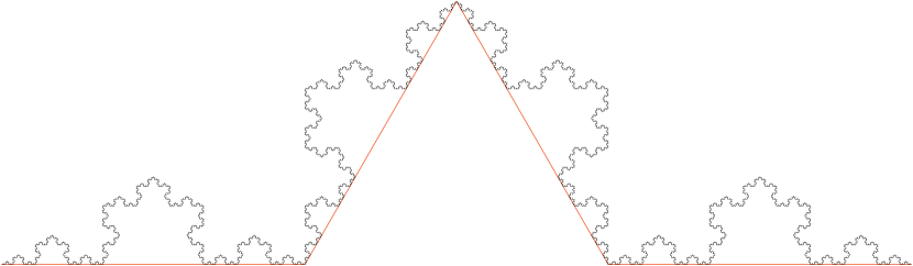
Figure 1: The Koch curve, obtained by repeatedly transforming a line segment. The result of the first transformation is shown as a broken line in red, to demonstrate the self similar structure more clearly. Each part of the Koch curve resting on the straight parts of this broken line is a smaller but an otherwise identical copy of itself.

Another way to obtain the fractal dimension is to measure the length of a curve in increasing detail. Since as we use smaller and smaller rulers, we will be resolving more and more detail; the measured length of the curve $L$, is a function of the ruler length $\varepsilon$ (Mandelbrot, 1967):

$$L(\varepsilon)\propto\varepsilon^{1-D}\,.$$ (1)

As an example, let us assume that we measure the length of the Koch curve by a given ruler and obtain $L_{0}$. When we reduce the ruler length by $1/3$, we shall be traversing the smaller copies in exactly the same manner we traversed the whole curve. Since there are four smaller copies, each of which will be measured to have a length $1/3$ times the whole curve, we have $L^{\prime}=4/3\times L$. To state in more general terms, if we modify our ruler length by $\varepsilon^{\prime}\leftarrow(1/m)\varepsilon$, the measured length changes by $L^{\prime}\leftarrow(n/m)L$. It is easy to see that this scaling is satisfied when $L\propto\varepsilon^{1-(\ln n/\ln m)}$. This method of determining the (fractal) dimension of a curve readily generalizes to real life curves, which are self similar only in a statistical sense (Mandelbrot, 1967).

For our purposes, it is more convenient to interpret a curve as the motion trail of an object. As we check the position of the object on this trail at decreasing time intervals, we will be resolving more details and the total trail length we calculate is going to increase. In other words, the trail length is going to be a function of the sampling interval $\chi$. For example, if we sample the motion of an object on the Koch curve $4$ times, we will be measuring the trail shown as the broken line in Figure 1, leading to an increase in length by $4/3$, with respect to going from the beginning to the end in one step. In more general terms, when the sampling interval is modified by $\chi^{\prime}\leftarrow(1/n)\chi$, the measured length becomes $L^{\prime}\leftarrow(n/m)L$. In this approach, the fractal dimension is determined through the relation

$$L(\chi)\propto\chi^{\frac{1}{D}-1}\,.$$ (2)

This technique of measuring fractal dimension of a trail can be easily applied to the results from dynamical simulations.

3 Simulations

3.1 Simulation Method and Parameters

The system we simulated has three components. At the centre lies a stationary supermassive black hole (SMBH) of mass $M_{\rm SMBH}=4\times 10^{6}M_{\sun}$. Around the SMBH, we have $N_{\rm field}=1200$ field stars each with mass $m_{\rm field}=2.5M_{\sun}$, semi-major axes distributed in a powerlaw cusp $M_{\rm cusp}(r)\propto r^{3/2}$ from $a_{\rm min}=0.0001$ to $a_{\rm max}=0.03\,{\rm pc}$, with eccentricities between $e_{\rm min}=0$ and $e_{\rm max}=0.95$, distributed following the distribution function $g(e)\propto e$. The final component is the massless test stars all with semimajor axis $a_{\rm test}=0.01\,{\rm pc}$, and eccentricities $e_{\rm test}=0.2$, $0.75$, and $0.85$ (12 stars each). Other orbital elements (inclination, longitude of the ascending node, argument of pericentre and mean anomaly) of all stars are picked at random. The exact values chosen do not matter too much, since over the course of the simulation the eccentricities are randomized. We chose these parameters to have a system that somewhat resembles the environment of S-stars observed at our Galactic centre. There are large uncertainties regarding the star distributions at this environment (Merritt, 2010, and references therein), and $t_{\rm dyn}\ll t_{\rm prec}\ll t_{\rm rlx}$ hierarchy may not even exist there. However, this condition would hold for a region around a SMBH that developed a Bahcall-Wolf cusp (Bahcall & Wolf, 1976, 1977), so we expect our method would be applicable to such systems.

The details of the code that is used for the simulations is going to be explained in detail elsewhere, here we point out only the key features. Both the field stars and the test stars feel the potential of the SMBH, including the general relativistic (GR) correction that leads to the prograde precession of the orbits. The test stars also feel the individual potential of the field stars, which leads to retrograde precession of their orbits and changes in angular momentum and energy. The field stars do not feel the individual potential of each other, but instead see the potential of a smooth cusp that is consistent with their distribution. This approximation decreases the time required for force computation significantly and was already employed by Rauch & Tremaine (1996) in their $N$-body simulations. For the interactions between the test stars and field stars we use a softening kernel ($\mathrm{K}_{2}$) of Dehnen (2001), with a softening length $10^{-4}$ pc. The units we adopted are $G=M_{\mathrm{field}}=3000M_{\sun}=1\,\mathrm{pc}=1$.

The extended mass distribution in the background cluster precesses the orbits in a retrograde fashion, and the GR effects lead to prograde precession. By our choice of parameters, these two effects cancel each other for a star with $a\sim 0.01\,\mathrm{pc}$ and $e\sim 0.6$. Mass precession becomes more effective as semi-major axes get larger and eccentricities get smaller, while the GR precession has the opposite behaviour.

We carry out the integration of the orbits using a high order Runge-Kutta-Nyström method, discovered by Blanes & Moan (2000, their SRKN${}^{b}_{11}$). We split the Hamiltonian into Keplerian and perturbation parts (Kinoshita et al., 1991) to increase efficiency and avoid spurious precession. This scheme advances the Keplerian orbital elements correctly, except for the truncation and the roundoff errors (the largest accumulated error per star amounts to $\sim 10^{-5}$ over the course of the whole simulation). In particular, the evolution of the Runge-Lenz vector does not exhibit a linear drift as in the case of potential energy-kinetic energy splitting (Hut et al., 1995). Our treatment of the GR perturbation leads to a small error in mean motion, but since we are interested in changes that take place over many orbits, this error is not important. We use shared adaptive timesteps, but time-symmetrize the integration with the method of Hut et al. (1995). Our simulations last 30 code units which corresponds to a few precession times of the slowest precessing test stars.

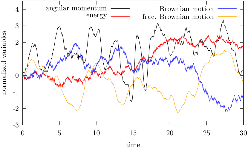
Figure 2: The evolution of angular momentum (black) and energy (red) for a test star with initial eccentricity $e_{0}=0.75$. For comparison, a Brownian motion (blue) and a fractional Brownian motion (yellow; $c=18$, $n=4000$) data as described in sec. 4 are also plotted. All curves are sampled at the same abscissae, and the ordinates are adjusted to have unit variance.

We record the energy and angular momentum of each test star throughout the simulation. In Figure 2 we show the evolution of these quantities for a star with initial eccentricity $e_{0}=0.75$. Even by eye, it is possible to tell that these quantities show a different behaviour. For comparison, in this figure we also plot the curves generated by Brownian and fractional Brownian motion, as described in Section 4.

3.2 Analysis of Simulation Results

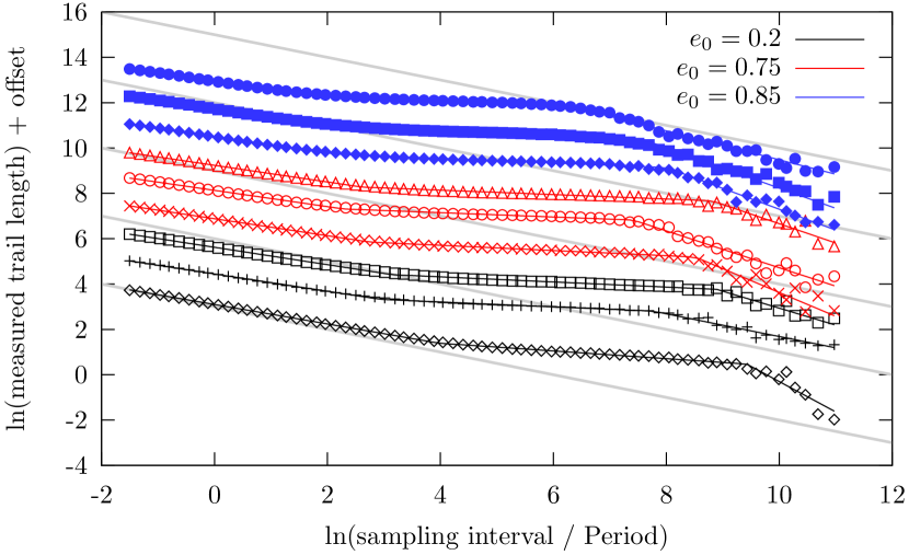
Figure 3: Measured trail lengths as a function of duration of the sampling intervals for angular momentum trails and the twice-broken power-law fits made to them. Sets are artificially offset from each other to avoid confusion. The gray lines in the background are to lead the eye and have slopes $-1/2$.

We measure the length of the angular momentum trail of each test star by sampling it at intervals ranging from the full length of the simulation down to a fraction of the orbital period. The dependence of the total measured trail length on the sampling interval is shown in Figure 3 for a few stars with different initial eccentricities. Starting from long sampling intervals and moving towards shorter ones, a number of features can be observed on this figure:

• For long timescales, the curves do not have the slope $-1/2$ (corresponding to dimension $D=2$, the value for Gaussian random walks (Mandelbrot, 1982)), but are somewhat steeper. This is to be expected since the energy of an orbit changes through relaxation and this process is much slower; hence the angular momentum evolution is bounded unlike a true random walk, and cannot be described by simple diffusion, even for long timescales.

• There is a marked transition to a more coherent motion as indicated by a decrease in the slope. The point of this transition can be determined with reasonable accuracy for a given star, but it is not common for all stars.

• Even though the slope decreases, it never becomes zero; hence the evolution of angular momentum is never ballistic ($\Delta L\not\propto\Delta t$).

• This slope can also be determined with reasonable accuracy for a given star, but varies from star to star.

• Looking at the eccentricity evolution of the stars reveals that the transition point is later for the stars that moved into $e\sim 0.6$ region where precession is slow. This is in harmony with the expectation that for more slowly precessing stars, the coherent torques last longer.

• The slope increases again for short timescales, but much before the period of the stars is reached. This randomization of the torques is a result of the stochastic nature of the processes that develop the torques and dominates the shorter timescale randomization that would result from orbital motion, at least down to the timescales we resolve.

Our results verify the presence of an intermediate regime, where the angular momentum evolution is enhanced. The evolution of angular momentum in this regime is not as rapid as ballistic growth $\Delta L\propto\Delta t$, but more rapid than diffusive growth $\Delta L\propto\Delta t^{1/2}$. This manner of evolution can be seen as the generalization of Brownian motion called fractional Brownian motion. Mandelbrot & van Ness (1968) describes various properties of this motion, along with applications. Mandelbrot (1982) gives further generalizations and methods to produce such curves. Even though these approaches are mathematically elegant and complete, in the next section we propose a simpler model that is easier to attach a physical interpretation.

4 A Simple Toy Model for Angular Momentum Evolution

One dimensional Brownian motion for a particle’s position $P(t)$ can be generated as follows. Let the motion over $\Delta t$ consist of $N$ steps with equal duration $\delta t=\Delta t/N$. We choose an initial value $P_{0}$ and at each step either increase or decrease the value of $P$ by $\delta P$. We decide which action to take by generating a sequence of random numbers $X_{i}$ uniformly sampled from the interval $[-0.5,0.5]$ and choosing a threshold value $q=0$. At each step, if $X_{i}<q$ we increase the value of $P$ and otherwise decrease it. To make the variance of the motion independent of the number of steps we choose $\delta P\propto 1/\sqrt{N}$. This scheme leads to Brownian motion (Gaussian random walk) for small $\delta t$, i.e, a large number of steps (Falconer, 2003, Chap. 16). It can be extended to a vector variable by letting each component perform independent Brownian motions.

We can introduce correlations between the increments of the variable $P$ by using a “repository”. For this, we keep track of the last $n$ values of $X_{i}$ and let our threshold value be proportional to their average $q=c\left<X_{i}\right>_{n}$, where $c$ is some constant. Here, $n$ determines the length of the correlations and $c$ determines their strength. We generated a few sets of data this way and measured the lengths of the resulting trails with differing sampling durations.

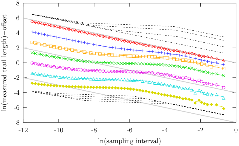
Figure 4: Measured trail lengths as a function of duration of the sampling intervals for various generated random walk data sets and the twice-broken power-law fits made to them. The set in the middle (green) has $c=18$, $n=4000$. The sets above it have varying $c=12,6,0$ and the sets below it have varying $n=2000,1000,500$ (see the text for explanation of these parameters). All sets have $N=200\,000$ points. To avoid confusion, sets are artificially offset from each other; but to make comparison easier, top four and bottom four sets are redrawn with dashed black lines at the top and bottom of the figure with identical offsets. The gray lines in the background are to lead the eye and have slopes $-1/2$.

The curves generated this way (Fig. 4) show very similar characteristics to angular momentum evolution. They exhibit an intermediate regime with lowered slope, whereas for long and short timescales the motion is more randomized. The upper bound of the intermediate regime is determined by the parameter $n$: the break occurs when the sampling interval matches $n\times\delta t$. The other parameter $c$ determines the slope in the intermediate and short timescale regime. Larger $c$ leads to a more coherent motion and a slope closer to $0$.

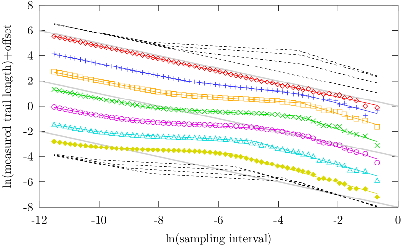
Figure 5: Same as Fig. 4 but for bounded random walks. The slopes for long sampling intervals are steeper than $-1/2$.

We also generated similar data with bounded random walks. For those, we started with a (vector) variable of unit magnitude $|\mathbf{P}(t=0)|=1$, and whenever a step led to $|\mathbf{P}|>1.5$, we took that step in the opposite direction. This limit roughly corresponds to the limit experienced by an orbit starting with initial eccentricity $e_{0}=0.75$, $J_{\mathrm{circular}}/J_{0}\sim 1.5$. The results from this bounded random walks are shown in Figure 5, exhibiting the long term correlations similar to angular momentum evolution.

5 Discussion

In this work, we studied the evolution of angular momentum in near-Keplerian systems by analyzing the outcome of $N$-body simulations. The simulation method we use incorporates certain approximations. Our test stars are massless, so they do not cause a back-reaction in the surrounding cluster. Furthermore, the field stars all have the same mass. A mass spectrum would change the granularity of the background potential, affecting the applied torques and possibly the coherence timescale. Finally, since the field stars do not see the granularity of their own potential, their angular momenta do not evolve. This decreases the rate of randomization of the background cluster, since vector resonant relaxation can change the orientation of the orbits on timescales comparable to mass and GR precession for some systems (for a comparison of these timescales for the Galactic centre, see Kocsis & Tremaine (2010)). If the torques on a star mainly change because of the rearrangement of the background cluster, rather than the reorientation of the orbit, this decrease in randomization would alter the rate of angular momentum evolution. All these approximations limit the domain of applicability of our $N$-body simulation approach; however, none of them alter the essential mechanism by which the angular momentum evolves.

We analyzed this evolution by calculating the fractal dimension of the angular momentum trail. With this method it is possible to reliably determine the onset of and the rate of evolution in different regimes. A key result of our analysis is that the evolution of angular momentum is neither diffusive nor ballistic in any regime, as was previously assumed in other studies (e.g. Hopman & Alexander, 2006; Eilon et al., 2009). This seems to contradict the results of the numerical experiments done by Rauch & Tremaine (1996). The reason for this discrepancy is not clear, but we speculate that it arises from the low number of stars used in that work.

We also developed a toy model that reproduces the features of angular momentum evolution. This model has adjustable parameters with clear physical interpretations. The relation between the appropriate values of these parameters and the physical variables requires more detailed and extensive analysis, which is currently underway. Apart from studying different initial conditions, we also plan to analyze the components of the torque parallel and perpendicular to the angular momentum separately. The nature of these torques can be very different (Rauch & Tremaine, 1996; Gürkan & Hopman, 2007), so a separate analysis should lead to a better understanding.

Koutsoyiannis (2002) developed fractional Gaussian noise generators (FGNGs) similar to our repository model. In that work he compares autoregressive moving average (ARMA) models to FGNGs, and finds that ARMA models are inferior for describing long-term correlations. These models need to be modified to have long term memory (Shumway & Stoffer, 2000), to describe angular momentum evolution in near-Keplerian systems. Alternatively, they can be used to describe short term correlations for torques, and long term correlations can be introduced by taking physical bounds into account, as is done here. After this paper was submitted, Madigan et al. (2010) also submitted a paper containing their analysis of this problem with ARMA models. They use ARMA(1,1) model, which fixes the value of the autocorrelation function for very large timescales to zero (see their figure 4) and hence does not lead to any correlations beyond a given time.

The computer programs used to generate and analyze the data are available from the author upon request.

References

- Alexander (2008) Alexander T., 2008, in S. K. Chakrabarti & A. S. Majumdar ed., AIP Conference Series Vol. 1053, The Galactic Center as a laboratory for extreme mass ratio gravitational wave source dynamics. p. 79
- Bahcall & Wolf (1976) Bahcall J. N., Wolf R. A., 1976, ApJ, 209, 214
- Bahcall & Wolf (1977) Bahcall J. N., Wolf R. A., 1977, ApJ, 216, 883
- Blanes & Moan (2000) Blanes S., Moan P. C., 2000, Journal of Computational and Applied Mathematics, 142, 313
- Dehnen (2001) Dehnen W., 2001, MNRAS, 324, 273
- Eilon et al. (2009) Eilon E., Kupi G., Alexander T., 2009, ApJ, 698, 641
- Falconer (2003) Falconer K. J., 2003, Fractal Geometry: Mathematical Foundations and Applications. John Wiley & Sons, West Sussex
- Gürkan & Hopman (2007) Gürkan M. A., Hopman C., 2007, MNRAS, 379, 1083
- Hopman & Alexander (2006) Hopman C., Alexander T., 2006, ApJ, 645, 1152
- Hut et al. (1995) Hut P., Makino J., McMillan S., 1995, ApJL, 443, L93
- Kinoshita et al. (1991) Kinoshita H., Yoshida H., Nakai H., 1991, Celestial Mechanics and Dynamical Astronomy, 50, 59
- Kocsis & Tremaine (2010) Kocsis B., Tremaine S., 2010, arXiv astro-ph, 1006.0001
- Koutsoyiannis (2002) Koutsoyiannis D., 2002, Hydrological Sciences Journal, 47, 573
- Madigan et al. (2010) Madigan A., Hopman C., Levin Y., 2010, arXiv astro-ph,1010.1535
- Madigan et al. (2009) Madigan A., Levin Y., Hopman C., 2009, ApJL, 697, L44
- Magorrian & Tremaine (1999) Magorrian J., Tremaine S., 1999, MNRAS, 309, 447
- Mandelbrot (1967) Mandelbrot B. B., 1967, Science, 156, 636
- Mandelbrot (1982) Mandelbrot B. B., 1982, The Fractal Geometry of Nature. Freeman, San Francisco
- Mandelbrot & van Ness (1968) Mandelbrot B. B., van Ness J. W., 1968, SIAM Review, 10, 422
- Merritt (2010) Merritt D., 2010, ApJ, 718, 739
- Rauch & Tremaine (1996) Rauch K. P., Tremaine S., 1996, New Astronomy, 1, 149
- Saha & Tremaine (1992) Saha P., Tremaine S., 1992, AJ, 104, 1633
- Shumway & Stoffer (2000) Shumway R. H., Stoffer D. S., 2000, Time Series Analysis and Its Applications. Springer-Verlag, New York
- Tremaine (1999) Tremaine S., 1999, in Impact of Modern Dynamics in Astronomy, IAU Colloquium 172, Resonant relaxation. p. 391
- Tremaine (2005) Tremaine S., 2005, ApJ, 625, 143