Resonance Parameters of the $\rho$-Meson from Lattice QCD

Abstract

We perform a nonperturbative lattice calculation of the P-wave pion-pion scattering phase in the $\rho$-meson decay channel using two flavors of maximally twisted mass fermions at pion masses ranging from 480 to 290 MeV. Making use of finite-size methods, we evaluate the pion-pion scattering phase in the center-of-mass frame and two moving frames. Applying an effective range formula, we find a good description of our results for the scattering phase as a function of the energy covering the resonance region. This allows us to extract the $\rho$-meson mass and decay width and to study their quark mass dependence.

I Introduction

In experiments, many hadrons are observed as resonances that decay via the strong interaction and have only a short life-time. On the theoretical side, the direct determination of the resonance parameters from QCD is afflicted with many difficulties since the computation of resonance masses and decay widths is essentially a nonperturbative problem. An attractive way to extract the resonance parameters nonperturbatively from first principles is the use of lattice QCD. Among unstable hadrons, the case of the $\rho$-meson is ideal for lattice studies of a resonance for two reasons. First, in lattice calculations, the noise-to-signal ratio in the computation of a meson mass is proportional to $e^{(m_{M}-m_{\pi})t}$, where $m_{M}$ is the meson mass under consideration, $m_{\pi}$ is the pion mass and $t$ is a typical hadronic time scale. Since the $\rho$ is one of the lightest mesons, the statistical error of its numerically computed mass can be well controlled. Second, the principle decay channel (with a branching rate of 99.9%) of the $\rho$-meson is to a pair of pions, which can be treated on the lattice very precisely.

In the past, several lattice groups have undertaken efforts to study the $\rho$-meson decay. A first attempt was made to estimate the decay width from the $\rho\rightarrow\pi\pi$ transition amplitude Gottlieb:1983rh ; Loft:1988sy ; McNeile:2002fh ; Jansen:2009hr . This method relies on two assumptions: first, the energy gap between the ground and the first excited state (corresponding to $\rho$-meson and $\pi\pi$ states with the same quantum numbers) is small. Second, it is assumed that the hadron interaction is not large and the transition amplitude $\langle\rho|\pi\pi\rangle$ satisfies $\langle\rho|\pi\pi\rangle\ll\langle\rho|\rho\rangle^{1/2}\langle\pi\pi|\pi\pi\rangle^{1/2}$. An alternative method, which does not rely on these assumptions, is to extract the $\rho$-meson resonance parameters from the P-wave pion-pion scattering phase in the isospin $I=1$ channel. The nonperturbative determination of the scattering phase is possible by using finite-size methods, which were originally proposed by Lüscher in the center-of-mass frame (CMF) Luscher:1985dn ; Luscher:1986pf ; Luscher:1990ck ; Luscher:1990ux ; Luscher:1991cf and later extended to more general cases employing also a moving frame (MF) by Rummukainen and Gottlieb Rummukainen:1995vs . Making use of these finite-size methods, two lattice studies Aoki:2007rd ; Gockeler:2008kc have been carried out to compute the $\rho$-meson resonance parameters. These calculations mainly concentrated on the scattering phase at one or two energies for a single ensemble. In this way, however, the scattering phase can be extracted at only a small number of energies and it becomes difficult to map out the resonance region.

In this work, we study the $I=1$ pion-pion scattering system using three Lorentz frames: the CMF, the first MF with total momentum ${\mathbf{P}}=(2\pi/L){\mathbf{e}}_{3}$ (MF1) and the second MF with ${\mathbf{P}}=(2\pi/L)({\mathbf{e}}_{1}+{\mathbf{e}}_{2})$ (MF2). Here, the ${\mathbf{e}}_{i}$ denotes a unit vector in the spatial direction $i$ and $L$ is the spatial extent of the lattice. In each frame, we evaluate the P-wave scattering phase from the energy eigenvalues of the ground state and the first excited state. Using three frames allows us to obtain the scattering phase at six energies for each set of physical parameters considered without the need to go to larger lattices. Therefore, we think that our calculations have two advantages compared to the earlier works mentioned above. First, extracting the resonance parameters from six energies allows us to obtain more accurate results. Second, some of the scattering phases are calculated at energies that lie in the range $[m_{\rho}-\Gamma_{\rho}/2,m_{\rho}+\Gamma_{\rho}/2]$, allowing us to directly map out the resonance region.

Our calculations are performed using the $N_{f}=2$ maximally twisted mass fermion ensembles Boucaud:2007uk ; Boucaud:2008xu ; Baron:2009wt from the European Twisted Mass Collaboration (ETMC) at a lattice spacing of $a=0.079~{}\mathrm{fm}$. The pion masses range from 290 up to 480 MeV, ensuring that the physical kinematics for the $\rho$-meson decay, $m_{\pi}/m_{\rho}<0.5$, is satisfied. The computation of the $\rho$-meson resonance parameters at several values of the pion mass allows us to obtain the pion mass dependence of the resonance mass and decay width and hence to perform an extrapolation to the physical point. The benefit of using twisted mass fermions is that at maximal twist physical observables are automatically accurate to $O(a^{2})$ in the lattice spacing, while the drawback is that isospin symmetry, although again an $O(a^{2})$ effect for the observables considered in this work, is broken at nonzero values of the lattice spacing. As a result, for any value of $a\neq 0$ the decay of $\rho^{0}$ to $\pi^{0}\pi^{0}$ is allowed, while in the continuum limit isospin symmetry is restored and this decay is forbidden. In this paper we present a first calculation to extract the $\rho$-meson resonance parameters from three Lorentz frames and discuss the feasibility and accuracy achievable using this setup. Since here we use only one value of the lattice spacing, we cannot test for the possible effects of isospin breaking. We plan to come back to this issue in the future when we will analyze gauge field ensembles obtained at finer values of the lattice spacing. As it will turn out, we are not able to match the high experimental accuracy of the $\rho$-meson resonance parameters with our lattice calculation. Still, we consider this work an important conceptual study and the techniques used here will be useful for other resonances such as the $\Delta$ baryon.

II Method

II.1 Scattering phase

In an elastic scattering system, the relativistic Breit-Wigner form (RBWF) for the scattering amplitude $a_{l}$ with a resonance at a center-of-mass (CM) energy $M_{R}$ and with a decay width $\Gamma_{R}$ is Amsler:2008zzb

$$a_{l}=\frac{-\sqrt{s}\Gamma_{R}(s)}{s-M_{R}^{2}+i\sqrt{s}\Gamma_{R}(s)}\;,\quad s=E_{CM}^{2}\;,$$

where $E_{CM}$ is the CM energy and $a_{l}$ is related to the scattering phase of the $l^{th}$ partial wave, $\delta_{l}$, through $a_{l}=(e^{2i\delta_{l}}-1)/2i$. The RBWF corresponding to $\delta_{l}$ is then

$$\tan\delta_{l}=\frac{\sqrt{s}\Gamma_{R}(s)}{M_{R}^{2}-s}\;.$$ (1)

The $\rho$-resonance has quantum numbers $I^{G}(J^{PC})=1^{+}(1^{--})$ and decays into two pions in the P-wave. A description of the scattering phase as a function of the $E_{CM}$ is provided by the effective range formula (ERF) Brown:1968zz

$$\tan{\delta_{1}}=\frac{g^{2}_{\rho\pi\pi}}{6\pi}\frac{p^{3}}{E_{CM}(m_{\rho}^{2}-E_{CM}^{2})}\;,\quad p=\sqrt{E_{CM}^{2}/4-m_{\pi}^{2}}\;,$$ (2)

which fits the experimental data well. In Eq. (2) $\delta_{1}$ is the P-wave pion-pion scattering phase, $g_{\rho\pi\pi}$ is the effective $\rho\rightarrow\pi\pi$ coupling constant and $m_{\rho}$ is the $\rho$-meson mass. We remark already at this point that we will use the ERF also for our lattice calculations to fit the scattering phase, even when using pion masses that are larger than the physical one. Comparing Eqs. (1) and (2), we find that the ERF is a particular case of the RBWF if the parameters $M_{R}$ and $\Gamma_{R}(s)$ are chosen such that

$$M_{R}=m_{\rho}\;,\quad\Gamma_{R}(s)=\frac{g^{2}_{\rho\pi\pi}}{6\pi}\frac{p^{3}}{s}\;.$$

The rho decay width $\Gamma_{\rho}$ can then be computed in the following way,

$$\Gamma_{\rho}=\Gamma_{R}(s)\Bigg{|}_{s=m_{\rho}^{2}}=\frac{g^{2}_{\rho\pi\pi}}{6\pi}\frac{p^{3}_{\rho}}{m_{\rho}^{2}}\;,\quad p_{\rho}=\sqrt{m_{\rho}^{2}/4-m_{\pi}^{2}}\;.$$ (3)

Thus Eqs. (2) and (3) allow us to extract $m_{\rho}$ and $\Gamma_{\rho}$ by studying the dependence of the pion-pion scattering phase $\delta_{1}$ on $E_{CM}$.

II.2 Finite-size methods

II.2.1 Center-of-mass frame

A direct calculation of the phase shift from lattice QCD is possible by using a finite-size method established by Lüscher Luscher:1985dn ; Luscher:1986pf ; Luscher:1990ck ; Luscher:1990ux ; Luscher:1991cf . In this method, the phase shift is obtained from the energy eigenvalues of a two-pion system enclosed in a cubic box with spatial size $L$.

In the CMF the possible energy eigenvalues for two noninteracting pions are given by

$$\bar{E}=2\sqrt{m_{\pi}^{2}+\bar{p}^{2}}\;,\quad\bar{p}=|\bar{\mathbf{p}}|\;,\quad\bar{\mathbf{p}}=(2\pi/L){\mathbf{n}}\;,\quad{\mathbf{n}}\in\mathbb{Z}^{3}\;.$$

In the interacting case the energy eigenvalues are shifted,

$$E=2\sqrt{m_{\pi}^{2}+p^{2}}\;,\quad p=(2\pi/L)q\;,$$

where $q$ is no longer constrained to originate from a quantized momentum mode. Because of the presence of the interaction, the energy eigenvalues deviate from those in the noninteracting case. It is exactly this deviation that contains the information of the underlying strong interaction and thus can be used to determine the scattering phase, as outlined next.

In this paper, we concentrate on the energy eigenstates with energies $E$ in the elastic region $2m_{\pi}<E<4m_{\pi}$ with the two-pion system having the same quantum numbers as the $\rho$-meson. In the CMF these states transform as a vector (more specifically the irreducible representation $\Gamma=T_{1}^{-}$) under the cubic group $O_{h}$. The corresponding finite-size formula connecting the energy $E$ to the scattering phase $\delta_{1}$ is given by Luscher:1991cf

$$\tan\delta_{1}(E)=\frac{\pi^{3/2}q}{\mathcal{Z}_{00}(1;q^{2})}\;,\quad\textmd{for }\;\Gamma=T_{1}^{-}\;,$$ (4)

with the zeta function defined through

$$\mathcal{Z}_{00}(s;q^{2})=\frac{1}{\sqrt{4\pi}}\sum_{{\mathbf{n}}\in\mathbb{Z}^{3}}\left(|{\mathbf{n}}|^{2}-q^{2}\right)^{-s}\;.$$

II.2.2 Moving frame

Using a MF with total momentum ${\mathbf{P}}=(2\pi/L){\mathbf{d}}$, ${\mathbf{d}}\in\mathbb{Z}^{3}$, the energy eigenvalues in the noninteracting case are given by

$$\bar{E}=\sqrt{m_{\pi}^{2}+\bar{p}_{1}^{2}}+\sqrt{m_{\pi}^{2}+\bar{p}_{2}^{2}}\;,$$

where $\bar{p}_{i}=|\bar{{\mathbf{p}}}_{i}|$ and $\bar{{\mathbf{p}}}_{i}$ denote the three-momenta of the pions, which satisfy the relations

$$\bar{{\mathbf{p}}}_{i}=(2\pi/L){\mathbf{n}}_{i}\;,\quad{\mathbf{n}}_{i}\in\mathbb{Z}^{3}\;,\quad\bar{{\mathbf{p}}}_{1}+\bar{{\mathbf{p}}}_{2}={\mathbf{P}}\;.$$ (5)

In the MF, the center-of-mass is moving with a velocity of ${\mathbf{v}}={\mathbf{P}}/\bar{E}$. Using the standard Lorentz transformation with a boost factor $\gamma=1/\sqrt{1-{\mathbf{v}}^{2}}$, the $\bar{E}_{CM}$ can be obtained as

$$\bar{E}_{CM}=\gamma^{-1}\bar{E}=2\sqrt{m_{\pi}^{2}+\bar{p}^{*2}}\;,$$

with CM momenta

$$\bar{p}^{*}=|\bar{\mathbf{p}}^{*}|\;,\quad\bar{\mathbf{p}}^{*}=\bar{\mathbf{p}}^{*}_{1}=-\bar{\mathbf{p}}^{*}_{2}=\frac{1}{2}\vec{\gamma}^{-1}(\bar{{\mathbf{p}}}_{1}-\bar{{\mathbf{p}}}_{2})\;.$$ (6)

Here, we use the notation

$$\vec{\gamma}^{-1}{\mathbf{p}}=\gamma^{-1}{\mathbf{p}}_{\parallel}+{\mathbf{p}}_{\perp}\;,\quad{\mathbf{p}}_{\parallel}=\frac{{\mathbf{p}}\cdot{\mathbf{v}}}{|\mathbf{v}|^{2}}{\mathbf{v}}\;,\quad{\mathbf{p}}_{\perp}={\mathbf{p}}-{\mathbf{p}}_{\parallel}\;.$$

From inspecting Eqs. (5) and (6) it can be seen that the $\bar{\mathbf{p}}^{*}$ are quantized to the values

$$\bar{\mathbf{p}}^{*}=(2\pi/L){\mathbf{n}}\;,\quad{\mathbf{n}}\in P_{\mathbf{d}}=\left\{{\mathbf{n}}\left|\;{\mathbf{n}}=\vec{\gamma}^{-1}({\mathbf{m}}+{\mathbf{d}}/2)\;,\;\;\textmd{for}\;{\mathbf{m}}\in\mathbb{Z}^{3}\right.\right\}\;.$$ (7)

In the interacting case, the $E_{CM}$ is given by

$$E_{CM}=2\sqrt{m_{\pi}^{2}+p^{*2}}\;,\quad p^{*}=(2\pi/L)q\;.$$ (8)

From the energy shift between the noninteracting and the interacting situation, $E_{CM}-\bar{E}_{CM}$ (or equivalently $q^{2}-|{\mathbf{n}}|^{2}$), one can compute the pion-pion scattering phase.

In the MF1 (${\mathbf{d}}={\mathbf{e}}_{3}$), the energy eigenstates transform under the tetragonal group $D_{4h}$. The irreducible representations $A_{2}^{-}$ and $E^{-}$ are relevant for the pion-pion scattering states $|\pi\pi,l=1\rangle$ in infinite volume with angular momentum $l=1$. In this work, we calculate the energies associated with the $A_{2}^{-}$ sector. The formula converting the $E_{CM}$ in a finite volume to the scattering phase in the infinite volume is given by Gottlieb and Rummukainen Rummukainen:1995vs as

$$\tan\delta_{1}(E_{CM})=\frac{\gamma\pi^{3/2}q}{\mathcal{Z}_{00}^{\mathbf{d}}(1;q^{2})+(2q^{-2}/\sqrt{5})\mathcal{Z}_{20}^{\mathbf{d}}(1;q^{2})}\;,\quad\textmd{for }\;\Gamma=A_{2}^{-}\;,$$ (9)

with the modified zeta function

$$\mathcal{Z}_{lm}^{\mathbf{d}}(s;q^{2})=\sum_{{\mathbf{n}}\in P_{\mathbf{d}}}\frac{\mathcal{Y}_{lm}^{*}({\mathbf{n}})}{\left(|{\mathbf{n}}|^{2}-q^{2}\right)^{s}}$$

and

$$\mathcal{Y}_{lm}(\mathbf{r})\equiv r^{l}Y_{l,m}(\Omega_{r})\;,\quad\mathcal{Y}_{l\bar{m}}(\mathbf{r})\equiv r^{l}Y_{l,-m}(\Omega_{r})\;,$$

where $\Omega_{r}$ represents the solid angle parameters ($\theta,\phi$) of $\mathbf{r}$ in spherical coordinates and the $Y_{l,m}$ are the usual spherical harmonic functions.

In order to obtain more energies in the resonance region, we developed a second moving frame (MF2) with ${\mathbf{d}}={\mathbf{e}}_{1}+{\mathbf{e}}_{2}$. The corresponding energy eigenstates transform under the orthorhombic group $D_{2h}$. The irreducible representations $B_{1}^{-}$, $B_{2}^{-}$ and $B_{3}^{-}$ occur for the $|\pi\pi,l=1\rangle$ states in infinite volume. Here we focus on the $B_{1}^{-}$ sector. Our derivation of the corresponding finite-size formula for the MF2 results in

$$\tan\delta_{1}(E_{CM})=\frac{\gamma\pi^{3/2}q}{\mathcal{Z}_{00}^{\mathbf{d}}-(q^{-2}/\sqrt{5})\mathcal{Z}_{20}^{\mathbf{d}}+i(\sqrt{3}q^{-2}/\sqrt{10})\left(\mathcal{Z}_{22}^{\mathbf{d}}-\mathcal{Z}_{2\bar{2}}^{\mathbf{d}}\right)}\;,$$

$$\hskip 270.30118pt\textmd{for }\;\Gamma=B_{1}^{-}\;.$$ (10)

For more details, we refer the reader to Ref. Feng:2011ah .

For brevity, we represent $\mathcal{Z}_{lm}^{\mathbf{d}}(1;q^{2})$ with the short notation $\mathcal{Z}_{lm}^{\mathbf{d}}$ in Eq. (II.2.2). Using Eqs. (4), (9) and (II.2.2) we can then convert a finite-volume determination of the $E_{CM}$ into a calculation of the P-wave scattering phase $\delta_{1}$. This is, of course, exactly the situation we are confronted with in a lattice calculation as performed here.

II.3 Correlation matrix

In the CMF, the value of the $E_{CM}$ is directly given by the discrete energy eigenvalue $E$ extracted from the large time behavior of the corresponding correlation function. In the MF, $E_{CM}$ is related to $E$ through the Lorentz transformation

$$E_{CM}^{2}=E^{2}-{\mathbf{P}}^{2}\;.$$ (11)

In order to calculate the energy eigenvalues $E$, we construct a $2\times 2$ correlation function matrix through

$$C_{2\times 2}(t)=\left(\begin{array}[]{cc}\left\langle\left(\pi\pi\right)(t)\;\left(\pi\pi\right)^{\dagger}(0)\right\rangle&\left\langle\left(\pi\pi\right)(t)\;\rho^{\dagger}(0)\right\rangle\\ \left\langle\rho(t)\;(\pi\pi)^{\dagger}(0)\right\rangle&\left\langle\rho(t)\;\rho^{\dagger}(0)\right\rangle\\ \end{array}\right)\;.$$ (12)

II.3.1 $\pi\pi$ sector

The $\pi\pi$ correlation function is constructed with the interpolating operators defined through

$$(\pi\pi)(t) = \frac{d_{\Gamma}}{N_{G}}\sum_{\hat{R}\in G}\chi_{\Gamma}(\hat{R})\left(\pi^{+}({\mathbf{P}}/2+\hat{R}{\mathbf{p}},t)\pi^{-}({\mathbf{P}}/2-\hat{R}{\mathbf{p}},t)\right.$$ (13)

$$\hskip 71.13188pt\left.-\pi^{-}({\mathbf{P}}/2+\hat{R}{\mathbf{p}},t)\pi^{+}({\mathbf{P}}/2-\hat{R}{\mathbf{p}},t)\right)\;,$$

with the momenta on the lattice $\mathbf{P}$ and ${\mathbf{p}}$ taking discrete values

$${\mathbf{P}}=(2\pi/L){\mathbf{d}}\;,\quad{\mathbf{p}}={\mathbf{P}}/2+(2\pi/L){\mathbf{m}}\;,\quad\textmd{for}\;\;{\mathbf{d}},{\mathbf{m}}\in\mathbb{Z}^{3}\;.$$

Let us explain the notation we have used in Eq. (13). The pion interpolating operator $\pi^{\pm}({\mathbf{q}},t)$ is defined through

$$\pi^{a}({\mathbf{q}},t)=\frac{1}{L^{3/2}}\sum_{\mathbf{x}}e^{-i{\mathbf{q}}\cdot{\mathbf{x}}}\left(\bar{\psi}\gamma_{5}\frac{\tau^{a}}{2}\psi\right)({\mathbf{x}},t)\;,\quad a=\pm,0\;,$$

where $\tau^{a}$ denote the isospin Pauli matrices and $\psi$ the two-flavor quark fields. We also introduce the symmetry group $G$ as the set of all lattice rotations and reflections $\hat{R}$, under which the set of $P_{\mathbf{d}}$ defined by Eq. (7) is invariant

$$G=\left\{\hat{R}\left|\;\hat{R}{\mathbf{n}}\in P_{\mathbf{d}}\;,\;\;\forall\;{\mathbf{n}}\in P_{\mathbf{d}}\right.\right\}.$$ (14)

In the CMF, MF1 and MF2, $G$ is given by the cubic groups $O_{h}$, $D_{4h}$ and $D_{2h}$, respectively. $\Gamma$ is the irreducible representation of the group $G$, $d_{\Gamma}$ is the dimension of $\Gamma$ and $\chi_{\Gamma}(\hat{R})$ is the character of $\Gamma$. The average over all the operations $\hat{R}$ in the group $G$ weighted by the coefficient $\chi_{\Gamma}(\hat{R})$ projects out the scattering states that belong to the $\Gamma$ representation. Finally, $N_{G}=\sum_{\hat{R}\in G}1$.

Given the momenta $\{{\mathbf{P}},{\mathbf{p}}\}$ and the representation $\Gamma$, one can construct the interpolating operators $(\pi\pi)(t)$ using Eq. (13). Here we set $\Gamma$ to be $T_{1}^{-}$, $A_{2}^{-}$ and $B_{1}^{-}$ for the CMF, MF1 and MF2, respectively, so that the energy eigenstates $|\pi\pi,\Gamma\rangle$ in finite volume will approximate the P-wave scattering states $|\pi\pi,l=1\rangle$ in infinite volume if one ignores states with higher angular momentum. In the CMF, the interpolating operator is given by

$$(\pi\pi)(t)=\pi^{+}\left(\frac{2\pi}{L}{\mathbf{e}}_{3},t\right)\pi^{-}\left(-\frac{2\pi}{L}{\mathbf{e}}_{3},t\right)-\pi^{+}\left(-\frac{2\pi}{L}{\mathbf{e}}_{3},t\right)\pi^{-}\left(\frac{2\pi}{L}{\mathbf{e}}_{3},t\right)\;.$$

In the two MFs, the operators are given in a unified form through

$$(\pi\pi)(t)=\pi^{+}\left({\mathbf{P}},t\right)\pi^{-}\left({\mathbf{0}},t\right)-\pi^{+}\left({\mathbf{0}},t\right)\pi^{-}\left({\mathbf{P}},t\right)\;,$$

with ${\mathbf{P}}$ again the total threa-momentum of the scattering system. We can use these operators to measure the energy eigenvalues $E$ from the corresponding correlation functions, convert $E$ into $E_{CM}$ by applying Eq. (11) and then extract the P-wave scattering phase $\delta_{1}$ using the finite-size formulae listed above.

II.3.2 $\rho$ sector

The interpolating operator for the neutral $\rho$-meson is constructed through a local vector current,

$$\rho(t)=\rho^{0}({\mathbf{P}},t)=\frac{1}{L^{3/2}}\sum_{{\mathbf{x}}}e^{-i{\mathbf{P}}\cdot{\mathbf{x}}}\left(\bar{\psi}({\mathbf{a}}\cdot{\mathbf{\gamma}})\frac{\tau^{0}}{2}\psi\right)({\mathbf{x}},t)\;,\quad{\mathbf{a}}\cdot{\mathbf{\gamma}}=\sum_{i=1}^{3}a_{i}\gamma_{i}\;,$$

where ${\mathbf{a}}$ indicates the polarization of the vector current. The direction of ${\mathbf{a}}$ is taken to be parallel to ${\mathbf{e}}_{3}$ in the CMF, ${\mathbf{e}}_{3}$ in the MF1 and ${\mathbf{e}}_{1}+{\mathbf{e}}_{2}$ in the MF2, respectively. This choice allows us to obtain a good signal-to-noise ratio for the off-diagonal matrix element $\left\langle\rho(t)\;(\pi\pi)^{\dagger}(0)\right\rangle$ in Eq. (12).

II.4 Extraction of energies

By computing the matrix of correlation functions in Eq. (12), we are able to isolate the ground state and first excited state in a clean way. This is of particular importance in the resonance region, where the avoided level crossing occurs and the first excited state is potentially close to the ground state. Such a situation renders the extraction of the ground state energy difficult when only a single exponential fit ansatz is used. Since we cannot predict a priori whether our energy levels will be close to the resonance region, we find it necessary to always use the correlation matrix to analyze our results. To extract the energy eigenstates, we follow the variational method Luscher:1990ck and construct a ratio of correlation function matrices as

$$R(t,t_{R})=C_{2\times 2}(t)C^{-1}_{2\times 2}(t_{R})\;,\quad\textmd{for}\;t>t_{R}\;,$$

where $t_{R}$, the reference time slice, is assumed to be large enough such that the contributions to the matrix $R(t,t_{R})$ from the excited states $|n\rangle$ with $n>2$ can be ignored.

The two eigenvalues $R_{n}(t,t_{R})$ ($n=1,2$) of the matrix $R(t,t_{R})$ behave as

$$R_{n}(t,t_{R})\rightarrow A_{n}\cosh\left(-E_{n}(t-T/2)\right)\;,$$ (15)

where we assume that $t$ is large enough ($t>t_{R}\gg 0$) to neglect excited states but still far enough from the boundaries ($t\ll T/2$) to ignore the unwanted thermal contributions as discussed in the case for the pion scattering length using twisted mass fermions in Ref. Feng:2009ij .

III Lattice calculation

III.1 Ensemble information

The results presented here are from a sequence of ensembles with a lattice spacing of $a=0.079~{}\mathrm{fm}$. The pion masses range from $m_{\pi}=480$ to $290~{}\mathrm{MeV}$. At all pion masses the physical kinematics of $m_{\pi}/m_{\rho}<0.5$ is satisfied, such that it is physically possible for the $\rho$-meson to decay into two pions. In our analysis we use two lattice sizes. The first corresponds to $L=1.9~{}\mathrm{fm}$ with pion masses of $m_{\pi}=480~{}\mathrm{MeV}$ and $m_{\pi}=420~{}\mathrm{MeV}$, i.e. ensembles $A_{1}$ and $A_{2}$ in Table 1. The second uses $L=2.5~{}\mathrm{fm}$ with pion masses of $m_{\pi}=330~{}\mathrm{MeV}$ and $m_{\pi}=290~{}\mathrm{MeV}$, i.e. ensembles $A_{3}$ and $A_{4}$ in Table 1. Additional information about the ensembles used is given in Table 1 and in Refs. Boucaud:2007uk ; Boucaud:2008xu ; Baron:2009wt .

Ensemble	$\beta$	$a\mu$	$L/a$	$m_{\pi}$	$m_{\pi}/m_{\rho}$	$N$
$A_{1}$	3.90	0.0085	$24$	480	0.43	176
$A_{2}$	3.90	0.0064	$24$	420	0.40	278
$A_{3}$	3.90	0.0040	$32$	330	0.32	124
$A_{4}$	3.90	0.0030	$32$	290	0.30	129

Table 1: Ensembles used in this work. We give the ensemble name $A_{i}$, the inverse bare coupling $\beta=6/g_{0}^{2}$, the bare quark mass $a\mu$, the lattice size $L/a$ and the value of $m_{\pi}$ in units of MeV. We also list the ratio $m_{\pi}/m_{\rho}$ and the number $N$ of configurations used.

III.2 Sources

To calculate the $\pi\pi$ correlation functions, we employ a stochastic method using $Z_{4}$ noise sources $\xi^{i}_{t_{s}}(\mathbf{x})$ that are restricted to each three-dimensional time-slice with time $t_{s}$. The sources $\xi^{i}_{t_{s}}(\mathbf{x})$ are also diluted in the color and spin indices, which are suppressed for simplicity. The index $i$ runs from $1$ to $N_{s}$, the number of stochastic noise sources. In this work we are able to achieve sufficient accuracy with just $N_{s}=1$ samples. Using the one-end trick Foster:1998vw , we need to introduce two stochastic noise sources, $e^{i{\mathbf{q}}\cdot{\mathbf{x}}}\xi^{i}_{t_{s}}(\mathbf{x})$ and $\xi^{i}_{t_{s}}(\mathbf{x})$, for each factor of $\pi^{\pm}({\mathbf{q}},t_{s})$ in the correlation function. For the correlation functions in the MFs, we must account for two momentum modes ($e^{i{\mathbf{q}}\cdot{\mathbf{x}}}\xi^{i}_{t_{s}}(\mathbf{x})$, ${\mathbf{q}}={\mathbf{0}}$ and ${\mathbf{q}}={\mathbf{P}}$). In the CMF there are three required momentum modes ($e^{i{\mathbf{q}}\cdot{\mathbf{x}}}\xi^{i}_{t_{s}}(\mathbf{x})$, ${\mathbf{q}}={\mathbf{0}}$, ${\mathbf{q}}=(2\pi/L){\mathbf{e}}_{3}$ and ${\mathbf{q}}=-(2\pi/L){\mathbf{e}}_{3}$). Since we place the source on all the time slices $t_{s}=0,\ldots,T\!-\!1$, we therefore perform $T$ inversions for each configuration and each momentum mode. Note that the time extent of our lattices is chosen to be always twice the spatial extent. The correlator $C_{11}(t)$ is then calculated through

$$C_{11}(t)=\left\langle\left(\pi\pi\right)(t)\left(\pi\pi\right)^{\dagger}(0)\right\rangle=\frac{1}{T}\sum_{t_{s}}\left\langle\left(\pi\pi\right)(t+t_{s})\left(\pi\pi\right)^{\dagger}(t_{s})\right\rangle\;.$$

The rather large effort to generate propagators on all the time slices allows us to obtain the correlators with high precision, which is important to extract the desired energies reliably.

In the calculation of the off-diagonal correlator, $C_{21}(t)$, the contraction of the quark fields leads to a three-point diagram. Since in this three-point diagram the two-pion fields are located at the same source time slice $t_{s}$, we use the sequential propagator method to construct the correlator. We calculate $C_{21}(t)$ through

$$C_{21}(t)=\left\langle\rho(t)(\pi\pi)^{\dagger}(0)\right\rangle=\frac{1}{T}\sum_{t_{s}}\left\langle\rho(t+t_{s})(\pi\pi)^{\dagger}(t_{s})\right\rangle\;,$$

and again average the correlator over all time slices $t_{s}$. For the second off-diagonal correlator $C_{12}(t)$, the two-pion fields are placed at the sink time slice $t+t_{s}$, which would render the computation of $C_{12}(t)$ more difficult. However, using the relation $C_{12}(t)=C_{21}^{\ast}(t)$, we get the off-diagonal matrix element $C_{12}$ for free.

For the $\rho$-correlator, $C_{22}(t)$, we have performed a comparison between the $Z_{4}$ stochastic source method and the point source method and found that the required computational effort to achieve a given signal-to-noise ratio is comparable. Historically, we started our work with the calculation of the hadronic vacuum polarization tensor Renner:2009by . Since in that work we generated point source propagators for the ensembles listed in Table 1, we just use the available propagators to construct the $\rho$-correlator

$$C_{22}(t)=\left\langle\rho^{\dagger}(t+t_{s})\rho(t_{s})\right\rangle\;,$$

where now the source time slices, $t_{s}$, are chosen randomly to reduce the autocorrelation between consecutive gauge field configurations.

Because of the isospin symmetry breaking effects at nonzero lattice spacing in our maximally twisted mass setup, the disconnected diagram for the neutral $\rho$-meson does not vanish. To address the disconnected contribution to the neutral $\rho$-meson, we need to generate, in principle, additional all-to-all propagators. However, the disconnected diagram correction has been studied in Ref. Michael:2007vn and has been found to be negligibly small, and hence we neglect it also here in the computation of the neutral $\rho$-correlator. For the same reason, we neglect the disconnected diagrams for the off-diagonal entries, where these contributions originate solely from the neutral $\rho$-operator. In the calculation of the correlator $\langle(\pi\pi)(\pi\pi)^{\dagger}\rangle$, we are able to address these disconnected pieces, since we put stochastic sources on all the time slices. We find that the disconnected diagram makes an apparently small contribution to the correlator but adds a significant amount of noise, which would destroy the signal for the connected piece. Therefore we drop it from the $\pi\pi$ sector. To be clear, neglecting these disconnected contributions is not a genuine approximation but is simply ignoring lattice artifacts that would vanish in the continuum limit anyway.

IV Results

IV.1 Energy eigenvalues

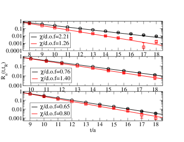
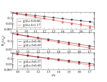
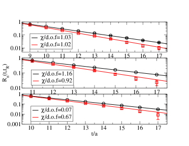
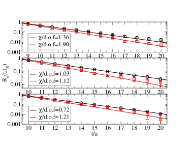
Figure 1: For the ensembles $A_{1}$ (upper left), $A_{2}$ (upper right), $A_{3}$ (lower left) and $A_{4}$ (lower right), the correlator $R_{n}(t,t_{R})$ ($n=1,2$) as a function of $t$ is shown. For each ensemble, from top to bottom the three plots present the lattice calculations in the CMF, MF1 and MF2, respectively. The solid lines are correlated fits to Eq. (15), from which the energy eigenvalues $E_{n}$ are extracted. In each plot, the upper curve is $n=1$ and the lower curve with the slightly steeper slope is $n=2$.

In Fig. 1 we show our lattice results for $R_{n}(t,t_{R})$ ($n=1,2$) in a logarithmic scale for the CMF, MF1 and MF2, as a function of time $t$ together with a correlated fit to the asymptotic form given in Eq. (15). From these fits we then extract the energies that will be used to determine the scattering phase. Note that the slopes of $\ln(R_{n}(t,t_{R}))$ are often very similar for $n=1$ and $n=2$, indicating that it is indeed essential to use the correlation function matrix. In order to extract the energies, we have to consider the two main sources of systematic error. One originates from the higher excited states and affects the correlator in the low-$t$ region. The other arises from the unwanted thermal contributions that distort the correlator in the large-$t$ region. By defining a fitting window $[t_{\mathrm{min}},t_{\mathrm{max}}]$ and varying the values of $t_{\mathrm{min}}$ and $t_{\mathrm{max}}$, we are able to control these systematic effects. In practice, we set $t_{\mathrm{min}}$ to be $t_{R}+1$ and increase the reference time slice $t_{R}$ to reduce the higher excited state contaminations. Besides this, we set $t_{\mathrm{max}}$ to be sufficiently far away from the time slice $t=T/2$ in order that the fitting results are protected from the unwanted thermal contributions. The corresponding parameters $t_{R}$, $t_{\mathrm{min}}$ and $t_{\mathrm{max}}$ used in this work are listed in Table 4. All the ensembles shown in Fig. 1 visibly agree with the corresponding fit and lead to reasonable values of $\chi^{2}/\mathrm{dof}$. The $\chi^{2}/\mathrm{dof}$ together with the fit results for $E_{n}$ ($n=1,2$) are also given in Table 4.

IV.2 Lattice discretization effects

In the continuum limit, the $E_{CM}$ is simply related to the energy spectrum $E_{n}$ through the Lorentz transformation of Eq. (11). However, on the lattice, the discretization effects explicitly break Lorentz symmetry and Eq. (11) is only valid up to discretization errors. Another discretization error arises from the continuum dispersion relation in Eq. (8), which is particularly relevant for the finite-size methods used here.

These two sources of systematic error have been studied in Ref. Rummukainen:1995vs , where the authors suggest to use the lattice modified relations

$$\cosh(E_{CM})=\cosh(E_{n})-2\sum_{i}\sin^{2}(P_{i}/2)\;,\quad n=1,2\;,$$

$$\cosh(E_{CM}/2)=2\sin^{2}(p^{*}/2)+\cosh(m_{\pi})\;,\quad p^{*}=(2\pi/L)q\;,$$ (16)

instead of the continuum relations to reduce these discretization errors. Following this suggestion, we calculate the energy $E_{CM}$ and the momentum $p^{*}$ from the energy eigenvalues $E_{n}$ using Eq. (IV.2) and then estimate the P-wave scattering phase $\delta_{1}$ by employing $p^{*}$ in the finite-size formulae. The results for $E_{CM}$, $p^{*}$ and $\delta_{1}$ are given in Table 5.

IV.3 Extraction of resonance parameters

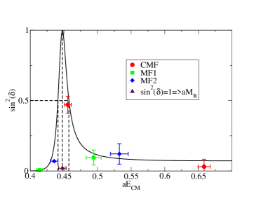
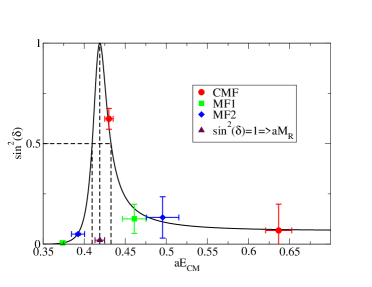
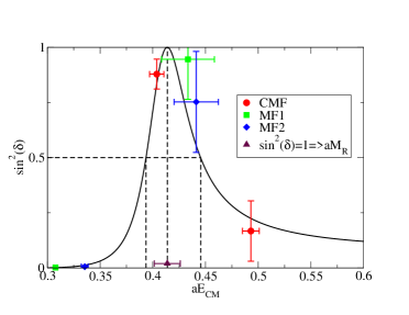
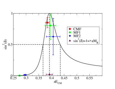
Figure 2: We show for the ensembles $A_{1}$ (upper left), $A_{2}$ (upper right), $A_{3}$ (lower left) and $A_{4}$ (lower right), the scattering phases calculated in the CMF, MF1 and MF2 together with the fits to the effective range formula Eq. (2). At the position where the scattering phase passes $\pi/2$, the resonance mass $m_{\rho}$ (denoted as $aM_{R}$ in the graph) is determined. Through the fit, the coupling constant $g_{\rho\pi\pi}$ and decay width $\Gamma_{\rho}$ are also extracted.

From the $E_{CM}$ we can now compute the P-wave scattering phases from six different energy levels, two from each of the three Lorentz frames employed. In order to extract the $\rho$-meson resonance parameters, we fit the results for the scattering phase to the effective range formula Eq. (2) and show the corresponding fits in Fig. 2. At the position where the scattering phase passes $\pi/2$, the resonance mass $m_{\rho}$ is determined. Additionally, the values of $g_{\rho\pi\pi}$ and hence $\Gamma_{\rho}$ are also evaluated from the fit. The corresponding results are given in Table 2.

	$m_{\pi}$ (MeV)	$m_{\rho}$ (MeV)	$\Gamma_{\rho}$ (MeV)	$g_{\rho\pi\pi}$
$A_{1}$	480	1118(14)	39.5(8.2)	6.46(40)
$A_{2}$	420	1047(15)	55(11)	6.19(42)
$A_{3}$	330	1033(31)	123(43)	6.31(87)
$A_{4}$	290	980(31)	156(41)	6.77(67)

Table 2: The results for the $\rho$-meson mass $m_{\rho}$, the decay width $\Gamma_{\rho}$ and the effective $\rho\rightarrow\pi\pi$ coupling $g_{\rho\pi\pi}$ at pion masses ranging from 480 to 290 MeV.

The finite-size methods are valid only for elastic scattering processes. In a situation with large enough energy, i.e. when $E_{CM}>4m_{\pi}$, the inelastic scattering channel will open and it is unclear how to the determine the scattering phase in such a case. Therefore, in our calculations we exclude results with energy $E_{CM}\gtrsim 4m_{\pi}$, which happened, fortunately, only for the excited state in the CMF for ensemble $A_{4}$.

IV.4 Comparison with other results

Using the resonance masses determined in the previous section, we show our values for $m_{\rho}$ together with those of other groups in Fig. 3 as a function of $m_{\pi}$. In order to compare these results, we scale $m_{\rho}$ and $m_{\pi}$ with the Sommer scale $r_{0}$ Sommer:1993ce as determined by the groups individually. This avoids systematic effects when determining the lattice spacing from different observables and is most appropriate when one aims only at a comparison of results between different groups. We find a rather satisfactory agreement and attribute the mild variation among the groups with possible residual cutoff and finite-size effects in the various calculations, although a definite conclusion cannot be given here.

We remark that our values of $m_{\rho}$ in physical units result from using the lattice spacing a=0.079 fm given earlier. This value of the lattice spacing was determined in Ref. Baron:2009wt by fixing the physical value of the pion decay constant $f_{\pi}$.

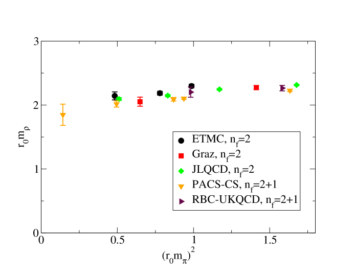
Figure 3: $\rho$-meson mass as function of the pion mass squared, both scaled with $r_{0}$. The $\rho$-meson resonance masses determined in our calculations (ETMC) are compared with those of the groups listed in the legend: chirally improved fermions (Graz) Gattringer:2008vj , overlap fermions (JLQCD) Aoki:2009qn ; Aoki:2008tq , nonperturbatively improved Wilson fermions (PACS-CS) Aoki:2008sm and domain wall fermions (RBC-UKQCD) Allton:2007hx ; Li:2006gra . In order to be consistent, we include only the results of those groups for which we could readily find the values of $r_{0}$ evaluated at the same coupling and pion mass as is the $\rho$-meson mass. Also, note that only our calculation includes a proper treatment of the resonance nature of the $\rho$-meson.

IV.5 Quark mass dependence

Having analyzed the ensembles listed in Table 1 allows us to discuss now the quark mass dependence of the $\rho$-meson resonance parameters. There are several works using effective field theory (EFT) to describe the quark mass dependence of the $\rho$-meson resonance parameters Jenkins:1995vb ; Bijnens:1997ni ; Leinweber:2001ac ; Bruns:2004tj ; Hanhart:2008mx . The general structure of the pion mass dependence of $m_{\rho}$ and $\Gamma_{\rho}$ can be written down as

$$m_{\rho} = M_{\rho}^{0}+C_{m1}M_{\pi}^{2}+C_{m2}M_{\pi}^{3}+O(M_{\pi}^{4})\;,$$

$$\Gamma_{\rho} = \Gamma_{\rho}^{0}+C_{\Gamma 1}M_{\pi}^{2}+C_{\Gamma 2}M_{\pi}^{3}+O(M_{\pi}^{4})\;.$$

However, before using these formulae, it should be realized that $m_{\rho}$ and $\Gamma_{\rho}$ are not only statistically correlated, but also inherently related to each other, suggesting that the coefficients $C_{mi}$ and $C_{\Gamma i}$ (i=1,2) are not independent from each other. Therefore, in this work we will follow the strategy of Refs. Djukanovic:2009zn ; Djukanovic:2010id where $m_{\rho}$ and $\Gamma_{\rho}$ are considered as the real and imaginary part of the complex pole of the $\rho$-meson propagator. Hence, we introduce the complex pole parameter $Z$ defined through

$$Z=(m_{\rho}-i\Gamma_{\rho}/2)^{2}\;.$$

In this approach the power counting is given by the complex-mass renormalization scheme. Up to $O(q^{4})$ in the chiral expansion, where $q$ is a typical pion momentum, $Z$ is given by Djukanovic:2009zn ; Djukanovic:2010id

$$Z = Z_{\chi}+C_{\chi}M_{\pi}^{2}-\frac{g^{2}_{\omega\rho\pi}}{24\pi}Z_{\chi}^{1/2}M_{\pi}^{3}$$

$$-\frac{g^{2}_{\omega\rho\pi}}{32\pi^{2}}M_{\pi}^{4}\left(\ln\frac{M_{\pi}^{2}}{M_{\chi}^{2}}-1\right)+\frac{g^{2}}{16\pi^{2}}\frac{M_{\pi}^{4}}{M_{\chi}^{2}}\left(3-2\ln\frac{M_{\pi}^{2}}{M_{\chi}^{2}}-2i\pi\right)\;,$$ (17)

where $Z_{\chi}=(M_{\chi}-i\Gamma_{\chi}/2)^{2}$ is the pole of the $\rho$-meson propagator in the chiral limit, $M_{\pi}^{2}$ is the lowest-order expression of the chiral expansion for the squared pion mass and $C_{\chi}$, $g_{\omega\rho\pi}$ and $g$ are coupling constants assuming real values. Using Eq. (17) to fit our results, we can determine the value of $Z$ at the physical point, where it can be converted to the physical resonance mass $m_{\rho,\mathrm{phy}}$ and decay width $\Gamma_{\rho,\mathrm{phy}}$.

In practice, we perform the chiral extrapolation of $Z$ in terms of the pion mass $m_{\pi}$ as extracted from the pseudoscalar correlation function as measured directly in the numerical calculations. By inserting the relation

$$m_{\pi}^{2}=M_{\pi}^{2}\left\{1+\frac{M_{\pi}^{2}}{32\pi^{2}F_{\pi}^{2}}\ln\frac{M_{\pi}^{2}}{\Lambda_{3}^{2}}+O(M_{\pi}^{4})\right\}$$

into Eq. (17), the expression for $Z$ in terms of $m_{\pi}$ is given by

$$Z = Z_{\chi}+C_{\chi}m_{\pi}^{2}-\frac{C_{\chi}m_{\pi}^{4}}{32\pi^{2}F_{\pi}^{2}}\ln\frac{m_{\pi}^{2}}{\Lambda_{3}^{2}}-\frac{g^{2}_{\omega\rho\pi}}{24\pi}Z_{\chi}^{1/2}m_{\pi}^{3}$$ (18)

$$-\frac{g^{2}_{\omega\rho\pi}}{32\pi^{2}}m_{\pi}^{4}\left(\ln\frac{m_{\pi}^{2}}{M_{\chi}^{2}}-1\right)+\frac{g^{2}}{16\pi^{2}}\frac{m_{\pi}^{4}}{M_{\chi}^{2}}\left(3-2\ln\frac{m_{\pi}^{2}}{M_{\chi}^{2}}-2i\pi\right)\;.$$

In Eq. (18) the values of the input parameters $F_{\pi}$ and $\Lambda_{3}$ are taken from Ref. Baron:2009wt with

$$F_{\pi}=\frac{1}{\sqrt{2}}f_{0}=86(1)~{}\mathrm{MeV}\;,\quad\ln\left(\Lambda_{3}^{2}/m^{2}_{\pi,\mathrm{phy}}\right)=\bar{l}_{3}=3.50(31)\;,$$

where $m_{\pi,\mathrm{phy}}$ is the physical pion mass.

Before we perform a precise test of Eq. (18), we first confront our lattice results with a simplified fit ansatz to order $O(q^{3})$, namely

$$Z=Z_{\chi}+C_{\chi}m_{\pi}^{2}-\frac{g^{2}_{\omega\rho\pi}}{24\pi}Z_{\chi}^{1/2}m_{\pi}^{3}\;.$$ (19)

Fit of $Z$ to	Eq. (19)	Eq. (18)
$m_{\rho,\mathrm{phy}}$	0.821(24)	0.850(35)
$\Gamma_{\rho,\mathrm{phy}}$	0.171(31)	0.166(49)
$M_{\chi}$	0.756(24)	0.803(47)
$\Gamma_{\chi}$	0.190(35)	0.179(58)
$C_{\chi}$	6.42(45)	4.9(2.0)
$g_{\omega\rho\pi}^{2}/24\pi$	9.8(1.5)	10(12)
$g^{2}/(16\pi^{2}M_{\chi}^{2})$	—	0.01(1.09)

Table 3: The physical $\rho$-meson mass and decay width as extracted using Eq. (19) and Eq. (18). The values of $m_{\rho,\mathrm{phy}}$, $\Gamma_{\rho,\mathrm{phy}}$, $M_{\chi}$ and $\Gamma_{\chi}$ are given in units of GeV and $g_{\omega\rho\pi}^{2}/24\pi$ and $g^{2}/(16\pi^{2}M_{\chi}^{2})$ are in units of $\mathrm{GeV}^{-2}$.

In the left panel of Fig. 4 we plot the mass of the $\rho$-meson as a function of the square of the pion mass together with a fit to Eq. (19). Using the fit to extrapolate to the physical point, our lattice result turns out to lie slightly high relative to the PDG value of the $\rho$-meson mass and shows a deviation of $1.9\,\sigma$.

In order to see whether higher-order corrections could reconcile our calculation with the experimentally determined $\rho$-meson mass, we also fit our lattice results to Eq. (18). All the fit results are listed in Table 3. From the simplified fit to Eq. (19) the lattice result of $g_{\omega\rho\pi}^{2}/24\pi$ is larger than the one suggested by EFT, which is $g_{\omega\rho\pi}^{2}/24\pi=3.4$ $\mathrm{GeV}^{-2}$ Leinweber:2001ac . After including the terms of $O(q^{4})$ in the fit, the uncertainty of the determination of $g_{\omega\rho\pi}^{2}/24\pi$ becomes, unfortunately, much larger and in fact $g_{\omega\rho\pi}^{2}/24\pi$ cannot be determined in a statistically significant way. A similar situation happens in the determination of the parameter $g^{2}/(16\pi^{2}M_{\chi}^{2})$. The KSFR relation Kawarabayashi:1966kd ; Riazuddin:1966sw

$$M_{\chi}^{2}=2g^{2}F_{\pi}^{2}$$

suggests that $g^{2}/(16\pi^{2}M_{\chi}^{2})$ takes the value of $1/(32\pi^{2}F_{\pi}^{2})=0.43$ $\mathrm{GeV}^{-2}$. However, we are unable to determine $g^{2}/(16\pi^{2}M_{\chi}^{2})$ reliably from the fit. As can be inferred from Table 3, using a fit to Eq. (18) there is a 40% uncertainty in the determination of $C_{\chi}$ and a more than 100% uncertainty in the determinations of both $g_{\omega\rho\pi}^{2}/24\pi$ and $g^{2}/(16\pi^{2}M_{\chi}^{2})$. Proceeding with these results, we plot the mass of the $\rho$-meson as a function of the square of the pion mass together with the fit to Eq. (18) in the right panel of Fig. 4. At the physical point the result of $m_{\rho}$ is still high relative to the PDG value, suggesting that the pion masses used in the current calculations are too high for even the $O(q^{4})$ extrapolations and that yet lighter quark masses will be necessary for quantitatively precise comparisons with experimental measurements of the $\rho$-meson mass.

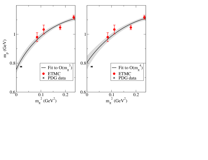
Figure 4: The $\rho$-meson resonance mass as a function of the square of the pion mass. In the left panel, we fit the lattice results to Eq. (19). In the right panel, we fit them to Eq. (18). Note that these are combined fits to $m_{\rho}$ and $\Gamma_{\rho}$ (shown in Fig. 6).

In Fig. 5, we plot the coupling $g_{\rho\pi\pi}$ as a function of the square of the pion mass and find that $g_{\rho\pi\pi}$ is practically independent of the pion mass. Moreover, the value of $g_{\rho\pi\pi}$ is consistent with the PDG value. This is not entirely unexpected. The coupling $g_{\rho\pi\pi}$, being dimensionless, is expected to be less sensitive to the pion masses and lattice spacings used in the calculation than the resonance mass $m_{\rho}$ is. In fact, whereas the accuracy of $m_{\rho}$ is currently systematically limited by the pion masses used in the calculation, the precision with which we can calculate $g_{\rho\pi\pi}$ is clearly dominated by just the statistical errors of the current calculation.

Eq. (3) shows that the decay width is determined from the fitted values of both $m_{\rho}$ and $g_{\rho\pi\pi}$. Hence, we expect that it will reflect a combination of the aspects just discussed. In fact, in the chiral limit Eq. (3) reduces to $\Gamma_{\rho}=m_{\rho}g^{2}_{\rho\pi\pi}/(48\pi)$. Thus the fact that $m_{\rho}$ overshoots the experimental measurement implies that $\Gamma_{\rho}$ will also be larger than the measured value. Additionally, the error of $g_{\rho\pi\pi}$ will be enhanced in $\Gamma_{\rho}$ leading to larger errors in the width than in the mass. These features can indeed be seen in Fig. 6, where we show the lattice results for $\Gamma_{\rho}$ as a function of the square of the pion mass together with the fit to Eq. (19) in the left panel and with the fit to Eq. (18) in the right panel. At the physical point, the decay widths are obtained as $\Gamma_{\rho,\mathrm{phy}}=171(31)~{}\mathrm{MeV}$ using the fit to Eq. (19) and as $\Gamma_{\rho,\mathrm{phy}}=166(49)~{}\mathrm{MeV}$ using the fit to Eq. (18). Both of the results are consistent with the PDG value $\Gamma_{\rho,\mathrm{PDG}}=149.1(0.8)~{}\mathrm{MeV}$ within 1$\sigma$. Note, however, that obviously the values determined from our lattice calculation are much less accurate than the one extracted from experimental measurements. Therefore, we consider the present work more as an initial study of how accurately resonance parameters can be extracted from nonperturbative lattice calculations and not as a precise determination of these parameters. The results we have obtained here demonstrate that resonances can indeed be analyzed on finite lattices with numerical calculations. This is very promising, given the number of hadrons that appear in the physical QCD spectrum as resonances.

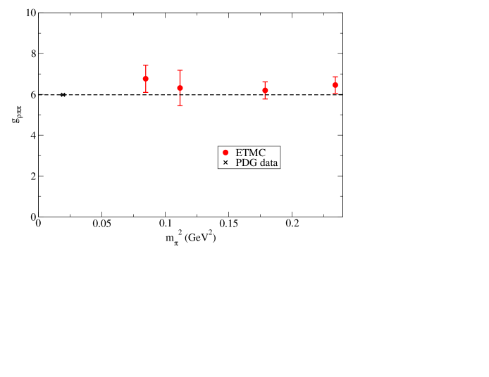
Figure 5: The effective coupling $g_{\rho\pi\pi}$ as a function of the square of the pion mass.

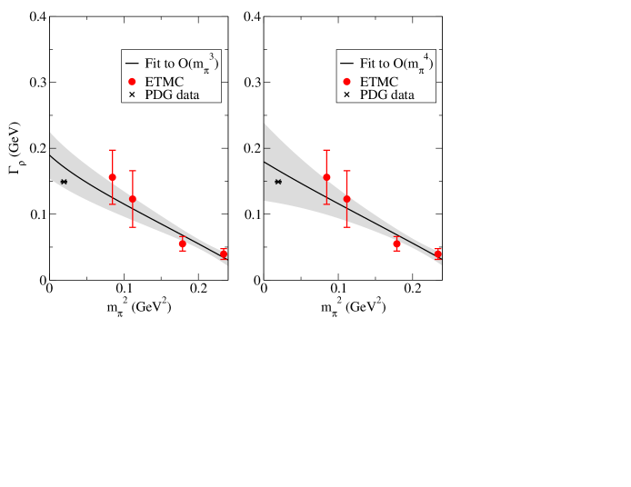
Figure 6: The $\rho$-meson decay width as a function of the square of the pion mass. The left panel shows the lattice results and the fit to Eq. (19). The right panel shows the fit to Eq. (18). Note that these are combined fits to $\Gamma_{\rho}$ and $m_{\rho}$ (shown in Fig. 4).

V Conclusion

In this work, we have calculated the P-wave pion-pion scattering phase in the $I=1$ channel near the $\rho$-meson resonance region. We have performed our calculations at pion masses ranging from $480$ to $290$ MeV and at a lattice spacing of $a=0.079$ fm. At all the pion masses, the physical kinematics for the $\rho$-meson decay, $m_{\pi}/m_{\rho}<0.5$, is satisfied. Compared to previous calculations, we have pushed the techniques much farther forward by employing three Lorentz frames simultaneously. This allowed us, in particular, to map out the energy region of the resonance without having to employ larger and more computationally demanding lattice calculations.

Making use of Lüscher’s finite-size methods, we evaluated the scattering phase from six energy eigenvalues per ensemble. In this way, we could fit the scattering phase with an effective range formula allowing us to extract the $\rho$-resonance mass $m_{\rho}$, the decay width $\Gamma_{\rho}$ and the effective coupling $g_{\rho\pi\pi}$. Taking the inherent relation between $m_{\rho}$ and $\Gamma_{\rho}$ into account, we have performed a fit to our results, obtained at four values of the pion mass, as a function of the complex parameter $Z=(m_{\rho}-i\Gamma_{\rho}/2)^{2}$. This provided a means of extrapolation to the physical point. Even though our fit formulae are guided by EFT, our results are not precise enough to perform a thorough test of the fit ansätze.

Keeping in mind the caveats just discussed, we quote for the $\rho$-meson mass $m_{\rho,\mathrm{phys}}=0.850(35)$ GeV and for the decay width $\Gamma_{\rho,\mathrm{phys}}=0.166(49)$ GeV. When these values are compared to the corresponding experimentally measured quantities, it is clear that the lattice computations cannot yet match the experimental accuracy. Although a precise determination of resonance parameters on the lattice is still a challenge, our work serves as a next step in the attempt to understand the strong decays in a conceptually clean way.

	Frame	$t_{R}/a$	$t_{\mathrm{min}}/a$	$t_{\mathrm{max}}/a$	n	$\chi^{2}/\mathrm{dof}$	$aE_{n}$
					1	2.21	0.4559(52)
	CMF	7	8	18	2	1.26	0.6584(90)
					1	0.76	0.4869(35)
$A_{1}$	MF1	9	10	18	2	1.40	0.5563(98)
					1	0.65	0.5660(42)
	MF2	8	9	18	2	0.80	0.642(11)
					1	0.66	0.4301(52)
	CMF	8	9	17	2	1.17	0.637(16)
					1	0.48	0.4537(25)
$A_{2}$	MF1	9	10	17	2	0.49	0.527(12)
					1	0.37	0.5343(57)
	MF2	9	10	17	2	0.40	0.612(16)
					1	1.03	0.4037(68)
	CMF	8	9	17	2	1.02	0.4931(80)
					1	1.16	0.3638(13)
$A_{3}$	MF1	10	11	17	2	0.92	0.474(23)
					1	0.07	0.4330(25)
	MF2	9	10	17	2	0.67	0.518(18)
					1	1.36	0.3844(79)
	CMF	8	9	20	2	1.90	0.4591(86)
					1	1.03	0.3363(14)
$A_{4}$	MF1	9	10	20	2	1.12	0.440(19)
					1	0.72	0.4035(36)
	MF2	9	10	20	2	1.21	0.490(22)

Table 4: Values of the energy eigenvalues for the ground state ($n=1$) and the first excited state ($n=2$) in the CMF, MF1 and MF2. In the table we list the ensemble number, the reference time $t_{R}$, the lower and upper bound of the fitting window, $t_{\mathrm{min}}$ and $t_{\mathrm{max}}$, the fit quality $\chi^{2}/\mathrm{dof}$ and the fit results for energy eigenvalues $E_{n}$ ($n=1,2$).

	Frame	$n$	$aE_{n}$	$aE_{CM}$	$ap^{*}$	$\delta_{1}(^{\circ})$
		1	0.4559(52)		0.1207(50)	137(3)
	CMF	2	0.6584(90)		0.2686(57)	170(9)
		1	0.4869(35)	0.4137(41)	0.0729(61)	4.7(.3)
$A_{1}$	MF1	2	0.5563(98)	0.494(11)	0.1543(91)	162(5)
		1	0.5660(42)	0.4356(56)	0.1000(62)	15.3(.4)
	MF2	2	0.642(11)	0.533(13)	0.1838(97)	160(6)
		1	0.4301(52)		0.1331(42)	128(3)
	CMF	2	0.637(16)		0.2719(96)	165(15)
		1	0.4537(25)	0.3737(31)	0.0794(36)	4.4(.1)
$A_{2}$	MF1	2	0.527(12)	0.461(14)	0.157(11)	159(6)
		1	0.5343(57)	0.3925(80)	0.0997(79)	12.9(.6)
	MF2	2	0.612(16)	0.495(20)	0.182(14)	159(9)
		1	0.4037(68)		0.1516(46)	70(6)
	CMF	2	0.4931(80)		0.2081(48)	156(10)
		1	0.3638(13)	0.3076(15)	0.0761(16)	2.4(.4)
$A_{3}$	MF1	2	0.474(23)	0.433(25)	0.171(16)	103(22)
		1	0.4330(25)	0.3354(33)	0.1013(27)	4(2)
	MF2	2	0.518(18)	0.441(21)	0.176(13)	120(15)
		1	0.3844(79)		0.1534(50)	67(7)
	CMF	2	$0.4591(86)^{*}$
		1	0.3363(14)	0.2743(17)	0.0726(15)	2.4(.3)
$A_{4}$	MF1	2	0.440(19)	0.396(22)	0.161(13)	116(16)
		1	0.4035(36)	0.2959(50)	0.0915(40)	6(2)
	MF2	2	0.490(22)	0.407(27)	0.167(17)	128(17)

Table 5: We give the P-wave scattering phase $\delta_{1}$ as extracted from the energies of the ground state and the first excited state in the CMF, MF1 and MF2. We list the ensemble number, the energies $E_{n}$ and $E_{CM}$, the momentum $p^{*}$ and the scattering phase $\delta_{1}$ (in units of degree). The single result marked by a star denotes that the corresponding $E_{CM}$ is above the $4m_{\pi}$ threshold. We therefore exclude that point from our calculations.

References

- (1) S. A. Gottlieb, P. B. Mackenzie, H. B. Thacker, and D. Weingarten. Phys. Lett., B134:346, 1984.
- (2) R. D. Loft and T. A. DeGrand. Phys. Rev., D39:2692, 1989.
- (3) C. McNeile and C. Michael. Phys. Lett., B556:177–184, 2003.
- (4) K. Jansen, C. McNeile, C. Michael, and C. Urbach. arXiv:0906.4720, 2009.
- (5) M. Luscher. Commun. Math. Phys., 104:177, 1986.
- (6) M. Luscher. Commun. Math. Phys., 105:153–188, 1986.
- (7) M. Luscher and U. Wolff. Nucl. Phys., B339:222–252, 1990.
- (8) M. Luscher. Nucl. Phys., B354:531–578, 1991.
- (9) M. Luscher. Nucl. Phys., B364:237–254, 1991.
- (10) K. Rummukainen and S. A. Gottlieb. Nucl. Phys., B450:397–436, 1995.
- (11) C.h. Kim, C.T. Sachrajda, and Stephen R. Sharpe. Nucl.Phys., B727:218–243, 2005.
- (12) Norman H. Christ, Changhoan Kim, and Takeshi Yamazaki. Phys.Rev., D72:114506, 2005.
- (13) S. Aoki et al. Phys. Rev., D76:094506, 2007.
- (14) M. Gockeler et al. arXiv:0810.5337, 2008.
- (15) S. Aoki et al. PoS, LATTICE2010:108, 2010.
- (16) J. Frison et al. arXiv:1011.3413, 2010.
- (17) Ph. Boucaud et al. Phys. Lett., B650:304–311, 2007.
- (18) Ph. Boucaud et al. Comput. Phys. Commun., 179:695–715, 2008.
- (19) R. Baron et al. JHEP, 08:097, 2010.
- (20) C. Amsler et al. Phys. Lett., B667:1, 2008.
- (21) L. S. Brown and R. L. Goble. Phys. Rev. Lett., 20:346–349, 1968.
- (22) Xu Feng, Karl Jansen, and Dru B. Renner. PoS, LAT2010:104, 2010.
- (23) X. Feng, K. Jansen, and D. B. Renner. Phys. Lett., B684:268–274, 2010.
- (24) M. Foster and Christopher Michael. Phys. Rev., D59:074503, 1999.
- (25) D. B. Renner and X. Feng. PoS, LATTICE2008:129, 2008.
- (26) C. Michael and C. Urbach. PoS, LAT2007:122, 2007.
- (27) R. Sommer. Nucl. Phys., B411:839–854, 1994.
- (28) C. Gattringer et al. Phys. Rev., D79:054501, 2009.
- (29) S. Aoki et al. Phys. Rev., D80:034508, 2009.
- (30) S. Aoki et al. Phys. Rev., D78:014508, 2008.
- (31) S. Aoki et al. Phys. Rev., D79:034503, 2009.
- (32) C. Allton et al. Phys. Rev., D76:014504, 2007.
- (33) Min Li. PoS, LAT2006:183, 2006.
- (34) E. E. Jenkins, A. V. Manohar, and M. B. Wise. Phys. Rev. Lett., 75:2272–2275, 1995.
- (35) J. Bijnens, P. Gosdzinsky, and P. Talavera. Nucl. Phys., B501:495–517, 1997.
- (36) D. B. Leinweber, A. W. Thomas, K. Tsushima, and S. V. Wright. Phys. Rev., D64:094502, 2001.
- (37) P. C. Bruns and U.-G. Meissner. Eur. Phys. J., C40:97–119, 2005.
- (38) C. Hanhart, J. R. Pelaez, and G. Rios. Phys. Rev. Lett., 100:152001, 2008.
- (39) D. Djukanovic, J. Gegelia, A. Keller, and S. Scherer. Phys. Lett., B680:235–238, 2009.
- (40) D. Djukanovic, J. Gegelia, A. Keller, and S. Scherer. arXiv:1001.1772, 2010.
- (41) K. Kawarabayashi and M. Suzuki. Phys. Rev. Lett., 16:255, 1966.
- (42) Riazuddin and Fayyazuddin. Phys. Rev., 147:1071–1073, 1966.