Power-law ensembles: fluctuations of volume or temperature ?

Abstract

We present two issues here: (i) that in situation when total energy is kept constant recently proposed fluctuations of volume ensemble is equivalent to the approach using Tsallis statistics with fluctuating temperature and (ii) that the later (in which fluctuations are described by the nonextensivity parameter $q$) leads to the observed experimentally sum rule connecting fluctuations of different physical observables.

1 Introduction

Statistical modelling represents a standard tool widely used to analyze multiparticle production processes [1]. However, this approach does not account for the possible intrinsic nonstatistical fluctuations in the hadronizing system which usually result in a characteristic power-like behavior of single particle spectra or in the broadening of the corresponding multiplicity distributions (and which can signal a possible phase transition(s) [2]). To include such features one should base this modelling on the so called Tsallis statistics [3, 4, 5] (represented by Tsallis distribution) which accounts for such situations by introducing, in addition to the temperature $T$, one new parameter, $q>1$, directly connected to fluctuations [6, 7] (for $q\rightarrow 1$ one recovers the usual Boltzmann-Gibbs distribution):

$$\exp_{q}\left(-\frac{E}{T}\right)=\left[1-(1-q)\frac{E}{T}\right]^{\frac{1}{1-q}}\,\stackrel{{\scriptstyle q\rightarrow 1}}{{\Longrightarrow}}\,\exp\left(-\frac{E}{T}\right),\qquad q-1=\frac{Var(1/T)}{\langle 1/T\rangle^{2}}.$$ (1)

The most recent applications of this approach come from PHENIX Collaboration at RHIC [8] and from CMS Collaboration at LHC [9]. One must admit at this point that this approach is subjected to a rather hot debate of whether it is consistent with the equilibrium thermodynamics or it is only a handy way to phenomenologically description of some intrinsic fluctuations in the system under consideration [10]. However, as was recently demonstrated on general grounds in [11], fluctuation phenomena can be incorporated into traditional presentation of thermodynamic and Tsallis distribution [3] belongs to the class of general admissible distributions which satisfy thermodynamical consistency conditions and which are therefore a natural extension of the usual Boltzman-Gibbs canonical distribution. Actually, what was shown in [6] was that starting from some simple diffusion picture of temperature equalization in the nonhomogeneous heat bath (in which local $T$ fluctuates from point to point around some equilibrium temperature, $T_{0}$) one gets evolution of $T$ in the form of Langevin stochastic equation and distribution of $1/T$, $f(1/T)$, as solution of the corresponding Fokker-Planck equation. It turns out that $f(1/T)$ has form of gamma distribution,

$$f(1/T)=\frac{1}{\Gamma\left(\frac{1}{q-1}\right)}\frac{T_{0}}{q-1}\left(\frac{1}{q-1}\frac{T_{0}}{T}\right)^{\frac{2-q}{q-1}}\cdot\exp\left(-\frac{1}{q-1}\frac{T_{0}}{T}\right).$$ (2)

Convoluting $\exp(-E/T)$ with such $f(1/T)$ one gets immediately Tsallis distribution, $\exp_{q}(-E/T)$ from Eq. (1) [6]. Parameter $q$, i.e., according to Eq. (1) also the temperature fluctuation pattern, is therefore fully given by the parameters describing this basic diffusion process (cf., [6] for details, this was recently generalized to account for the possibility of transferring energy from/to heat bath, which appears to be important for AA applications [4, 12] and for cosmic ray physics [13]; we shall not discuss this issue here). This approach has now been successfully applied in many circumstances, see [4, 12, 8, 9] and references therein.

2 Fluctuations of $V$ or $T$?

It must be stressed at this point that the form of $f(1/T)$ as given by Eq. (2) is not assumed but has been derived from the underlying physical process. We shall now compare this approach with that proposed in [14] in which the volume $V$ was assumed to fluctuate in the scale invariant way following the observed KNO scaling behavior of the multiplicity distributions, $P(N)$ [15]. We shall demonstrate here that when total energy is kept constant, as was assumed in [14], both approaches are equivalent. Let us first notice that for constant total energy, $E=const$, both the volume $V$ and temperature $T$ are related via $E\sim VT^{4}$, what means that

$$T=\langle T\rangle\left(\frac{\langle V\rangle}{V}\right)^{\frac{1}{4}}=\frac{\langle T\rangle}{y}\quad{\rm where}\quad y=\left(\frac{V}{\langle V\rangle}\right)^{\frac{1}{4}}.$$ (3)

Following now [14] the mean multiplicity in the microcanonical ensemble (MCE), $\bar{N}$, can be written as

$$\bar{N}=\langle N\rangle\cdot\frac{V}{\langle V\rangle}\left(\frac{T}{\langle T\rangle}\right)^{3}\ =\ \langle N\rangle\ y,$$ (4)

what means that $\bar{N}$ fluctuates in the same way $y$. It is then natural to assume that $y$ follows the pattern of fluctuations of $\bar{N}$, i.e., KNO limit of the NBD distribution observed in data fitting [15], which is given by gamma function. The power-like form of single particle spectra then follow immediately, all apparently without invoking any reference to Tsallis statistics. Notice, however, that because of (3), $1/T$ will fluctuate according to the same gamma distribution. So we get $T$ fluctuations with the same functional form but now without the physical background behind the Eq. (2) mentioned above. However, we can proceed in reverse order and obtain from our $T$ fluctuations introduced in Section 1 fluctuations of $V$ introduced in [14]. In this sense both approaches are equivalent with the former being based on some physical processes and the second on apparently ad hoc assumption.

We close this section with short reminder that temperature fluctuations discussed in Section 1 result in automatic broadening of the corresponding multiplicity distributions, $P(N)$, from the poissonian form for exponential distributions to the negative binomial (NB) form for Tsallis distributions [17]. It is known that whenever we have $N$ independently produced secondaries with energies $\{E_{i=1,\dots,N}\}$ taken from the exponential distribution in Eq. (1) and whenever $\sum^{N}_{i=0}E_{i}\leq E\leq\sum^{N+1}_{i=0}E_{i}$, then the corresponding multiplicity distribution is poissonian,

$$P(N)=\frac{\left(\bar{N}\right)^{N}}{N!}\exp\left(-\bar{N}\right)\quad{\rm where}\quad\bar{N}=\frac{E}{\lambda}.$$ (5)

What was shown in [17] is that whenever in some process $N$ particles with energies $\{E_{i=1,\dots,N}\}$ are distributed according to the joint $N$-particle Tsallis distribution,

$$h\left(\{E_{i=1,\dots,N}\}\right)\!=\!C_{N}\left[1-(1-q)\frac{\sum^{N}_{i=1}E_{i}}{\lambda}\right]^{\frac{1}{1-q}+1-N}$$ (6)

(for which the corresponding one particle Tsallis distribution function in Eq. (1), is marginal distribution), then, under the same condition as above, the corresponding multiplicity distribution is the NB distribution,

$$P(N)\,=\,\frac{\Gamma(N+k)}{\Gamma(N+1)\Gamma(k)}\frac{\left(\frac{\langle N\rangle}{k}\right)^{N}}{\left(1+\frac{\langle N\rangle}{k}\right)^{(N+k)}};\quad{\rm where}\quad k=\frac{1}{q-1}.$$ (7)

Notice that in the limiting cases of $q\rightarrow 1$ one has $k\rightarrow\infty$ and (7) becomes a poissonian distribution (5), whereas for $q\rightarrow 2$ on has $k\rightarrow 1$ and (7) becomes a geometrical distribution. It is easy to show that for large values of $N$ and $\langle N\rangle$ one obtains from Eq. (7) its scaling form,

$$\langle N\rangle P(N)\cong\psi\left(z=\frac{N}{\langle N\rangle}\right)=\frac{k^{k}}{\Gamma(k)}z^{k-1}\exp(-kz),$$ (8)

in which one recognizes a particular expression of Koba-Nielsen-Olesen (KNO) scaling [15] and which, as discussed before, has been assumed to describe also the volume fluctuations in [14]. Here it results from the temperature fluctuations described by the parameter $q$ discussed in Section 1 with well defined physical meaning.

3 Composition of different fluctuations

Description of fluctuations phenomena by means of the parameter $q$ using Tsallis statistics allows for better understanding of interrelations between different fluctuations. From our experience with $p{\bar{p}}$ collisions [19] we know that one can obtain very good description of the whole range of $p_{T}$ ($\propto\exp_{q}\left(-p_{T}/T\right)$ with $(T_{T}$ [GeV]$;q_{T})=(0.134;1.095)$, $(0.135;1.105)$ and $(0.14;1.11)$ for energies (in GeV) $200$, $540$ and $900$, respectively. These values should be compared with the corresponding values of $(T=T_{L};q=q_{L})$ obtained when fitting rapidity distributions ($\propto\exp_{q}\left(-\mu_{T}\cosh y/T\right)$) at the same energies: $(11.74;1.2)$, $(20.39;1.26)$ and $(30.79;1.29)$. It was noticed there that $q_{L}-1$ has the same energy behavior as $1/k$ in the NB distribution fitting the multiplicity distributions at corresponding energies ($q_{L}-1=-0.104+0.058\ln\sqrt{s}$). It means that fluctuations of total energy are in this case driven mainly by fluctuations in the longitudinal phase space. Explanations proposed in [19] was following. Noticing that $q-1=\sigma^{2}(T)/T^{2}$ (i.e., it is given by fluctuations of total temperature $T$) and assuming that $\sigma^{2}(T)=\sigma^{2}(T_{L})+\sigma^{2}(T_{T})$, one can estimate that resulting values of $q$ should not be too different from

$$q\,=\,\frac{q_{L}\,T_{L}^{2}\,+\,q_{T}\,T^{2}_{T}}{T^{2}}\,-\,\frac{T^{2}_{L}\,+\,T^{2}_{T}}{T^{2}}\,+\,1\quad\stackrel{{\scriptstyle T_{L}\gg T_{T}}}{{\Longrightarrow}}\quad\sim q_{L}.$$ (9)

It turns out that situation is completely reversed in the case of nuclear collisions, which we shall discuss now, cf. Fig. 1. Left panel shows $q$ obtained from different sources as function of centrality represented by number of participants, $N_{P}$. The one obtained from $P(N)$ follows

$$q-1=\frac{1}{aN_{P}}\left(1-\frac{N_{P}}{A}\right)$$ (10)

behavior ($a=0.98$) [12]. Whereas for small centralities it approaches situation encountered in $p\bar{p}$ collisions (where it was practically equal to $q=q_{L}$ obtained from rapidity distributions as mentioned above), the more central is event the smaller is $q-1$, i.e., the nearer to poissonian is the corresponding $P(N)$. Notice that both, $q_{L}$ and $q_{T}$ (obtained from $p_{T}$ distributions are now greater than $q$ and have (approximately) visible similar dependence on $N_{P}$, however now $q_{L}<q_{T}$, again opposite to what was seen in $p\bar{p}$ [19] (for comparison $q_{T}$ obtained by [21] using RHIC data $Au+Au$ collisions at $200$ GeV [22] are shown here as well). Right panel shows the same quantities but now as function of energy for the most central $Pb+Pb$ collisions [20]. In both cases we take from [20] distributions of rapidity, $dN/dy$, and in $\mu_{T}$, $dN/d\mu_{T}$, and from them deduces the corresponding $q$.

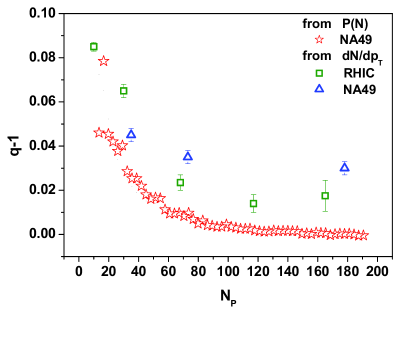
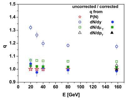
Figure 1: Left panel: $q$ from $P(N)$ are our results obtained in [12] from $Var(N)/\langle N\rangle$, $q$ from RHIC are taken from compilation [21] and are based on data for $dN/dp_{T}$ from [22] analyzed there, whereas $q$ from NA49 are obtained by us for this presentation using data on $dN/dp_{T}$ from the first work in [20]. Right panel: all results were obtained for the sake of this presentation using distributions provided by [20], i.e., respectively, $dN/d\mu_{T}$, $dN/dy$ and $dN/dp_{T}$. The errors are similar to those presented as example for $q$ obtained from $dN/dy$. Open symbols correspond to uncorrected values of $q$, full symbols to values corrected by means of the procedure proposed in the text.

The natural question is, what causes such different behavior of parameter $q$ in this case. The answer we propose is the following. When extracting values of parameter $q$ from the rapidity distributions tacit assumption was made that $\mu_{T}$ in $E=\mu_{T}\cosh y$ remains constant (i.e., it does not fluctuate). What would happen if this assumption was false? Notice that in the $\exp_{q}\left(-E/T\right)=exp_{q}\left[-\left(\mu_{T}/T\right)\cosh y\right]=\exp_{q}(-z\cosh y)$. It means that fits to rapidity distributions provide us, in fact fluctuations not so much of partition temperature $T$ but rather of the variable $z=\mu_{T}/T$. This in turn can be written approximately as:

$$Var(z)\simeq\frac{1}{\langle T\rangle^{2}}Var\left(\mu_{T}\right)+\frac{\langle\mu_{T}\rangle^{2}}{\langle T\rangle^{2}}\cdot\frac{Var(T)}{\langle T\rangle^{2}}.$$ (11)

Because $\langle z\rangle\simeq\langle\mu_{T}\rangle/\langle T\rangle$ and $Var(1/T)/\langle 1/T\rangle^{2}\simeq Var(T)/\langle T\rangle^{2}$ and because $Var(z)/\langle z\rangle^{2}=Var\left(\mu_{T}\right)/\langle\mu_{T}\rangle^{2}+Var(T)/\langle T\rangle^{2}$ one can write that

$$q-1\stackrel{{\scriptstyle def}}{{=}}\frac{Var(T)}{\langle T\rangle^{2}}=\frac{Var(z)}{\langle z\rangle^{2}}-\frac{Var\left(\mu_{T}\right)}{\langle\mu_{T}\rangle^{2}}.$$ (12)

This sum rule is our main result and its action is presented in the right panel of Fig. 1. It connects total $q$, which can be obtained from the analysis of the NB form of the measured multiplicity distributions, P(N), with $q_{L}-1=Var(z)/\langle z\rangle^{2}$, obtained from fitting rapidity distributions and $Var\left(\mu_{T}\right)/\langle\mu_{T}\rangle^{2}$ obtained from data on transverse mass distributions. When extracting $q$ from distributions of $dN/d\mu_{T}$ we proceed in analogously way with $z$ being in this case equal to $z=\cosh y/T$.

4 Summary

To summarize: we have demonstrated that for constant total energy fluctuations of $T$ introduced by us some time ago [6, 4] are equivalent to fluctuations of $V$ proposed recently [14] and that, at the moment, the former have advantage of being backed by a plausible physical arguments [6]. Moreover, due to relation (3) valid for constant total energy, the inverse temperature $1/T$ and $V^{1/4}$ fluctuate in the same way, according to gamma distribution and such fluctuations lead to the Tsallis form of the respective distributions for energy spectra.

However, the main results presented here is the sum rule formula, Eq. (12), connecting $q$ obtained from analysis of different distributions which are obtained in the same experiment. This allows us to understand why in $AA$ collisions fluctuations observed in multiplicity distributions are much smaller than the corresponding ones seen in the rapidity distribution or in distribution of transverse momenta (i.e., why the corresponding $q$ parameters evaluated from distributions of different observables are different). This issue should be checked further when completely sets of data would become available from the experiments at LHC (especially from ALICE).

References

- [1] See, for example, M. Gaździcki, M. Gorenstein and P. Seybothe, arXiv:1006.1765[hep-ph], and references therein.
- [2] L. Stodolsky, Phys. Rev. Lett. 75 (1995) 1044; H. Heiselberg, Phys. Rep. 351 (2001) 161; S. Mrówczyński, Acta Phys. Pol. B 40 (2009) 1053.
- [3] C. Tsallis, Eur. Phys. J. A 40 257, for an updated bibliography on this subject see http://tsallis.cat.cbpf.br/biblio.htm.
- [4] G. Wilk and Z Włodarczyk, Eur. Phys. J. A 40 (2009) 299.
- [5] T. S. Biró, G. Purcel and K. Ürmösy, Eur. Phys. J. A 40 (2009) 325.
- [6] G. Wilk and Z. Włodarczyk, Phys. Rev. Lett. 84 (2000) 2770.
- [7] T. S. Bir o and A. Jakov ac, Phys. Rev. Lett. 94 (2005) 132302.
- [8] A. Adare et al. (PHENIX Coll.), arXiv:1005.3674[hep-exp], to be published in Phys. Rev. D.
- [9] V. Khachatryan et al., (CMS Collaboration), JHEP02 (2010) 041.
- [10] M. Nauenberg, Phys. Rev. E 67 (2003) 036114 and Phys. Rev. E 69 (2004) 038102; C. Tsallis, Phys. Rev. E 69 (2004) 038101; R. Balian and M. Nauenberg, Europhys. News 37 (2006) 9; R. Luzzi, A. R. Vasconcellos and J. Galvao Ramos, Europhys. News 37 (2006) 11.
- [11] O. J. E. Maroney, Phys. Rev. E 80 (2009) 061141.
- [12] G. Wilk and Z Włodarczyk, Phys. Rev. C 79(2009) 054903.
- [13] G. Wilk and Z Włodarczyk, Cent. Eur. J. Phys. 8 (2010) 726.
- [14] V. V. Begun, M. Gaździcki and M. I. Gorenstein, Phys. Rev. C 7̱8, (2008) 024904.
- [15] Z. Koba, H. B. Nielsen and P. Olesen, Nucl. Phys. B 40 (1972) 319.
- [16] G. Alexander et al. (OPAL Coll.), Z. Phys. C 72 (1996) 389; G. Giacomelli, Nucl. Phys. Proc. Suppl. B B25 (1991)30; A. Breakstone et al., Phys. Lett. B 162 (1985) 400.
- [17] G. Wilk and Z. Włodarczyk, Physica A 376 (2007) 279.
- [18] M. Rybczyński, Z. Włodarczyk and G. Wilk, Nucl. Phys. B (Proc. Suppl.) 1̱22 (2003) 325; F. S. Navarra, O. V. Utyuzh, G. Wilk, and Z. Włodarczyk, Phys. Rev. D 67 (2003) 114002.
- [19] F. S. Navarra, O .V. Utyuzh, G. Wilk and Z. Włodarczyk, Physica A 340 (2004) 467.
- [20] C. Alt et al., Phys. Rev. C 77 (2008) 034906; C. Alt et al., Phys. Rev. C 77 (2008) 024903 (2008); S. V. Afanasiev et al., Phys. Rev. C 66 (2002) 054902.
- [21] Ming Shao, Li Yi, Zebo Tang, Hongfang Chen, Cheng Li and Zhangbu Xu, J. Phys. G 37 (2010) 085104.
- [22] S. S. Adler et al. (PHENIX Coll.), Phys. Rev. C 71 (2005) 034908 (2005).