Investigation of the $\Lambda_{b}\rightarrow\Lambda\ell^{+}\ell^{-}$ transition in universal extra dimension using form factors from full QCD

Using the related form factors from full QCD which recently are available, we provide a comprehensive analysis of the $\Lambda_{b}\rightarrow\Lambda\ell^{+}\ell^{-}$ transition in universal extra dimension model in the presence of a single universal extra dimension called the Applequist-Cheng-Dobrescu model. In particular, we analyze some related observables like branching ratio, forward-backward asymmetry, double lepton polarization asymmetries and polarization of the $\Lambda$ baryon in terms of compactification radius and corresponding form factors. We present the sensitivity of these observables to the compactification parameter, $1/R$ up to $1/R=1000~{}GeV$. We also compare the results with those obtained using the form factors from heavy quark effective theory as well as the SM predictions.

PACS number(s): 12.60-i, 13.30.-a, 13.30.Ce ,14.20.Mr

1 Introduction

The Standard Model (SM) of particle physics describes all known particles and their interactions except than gravity. The SM is the only minimal model which is in perfect consistency with all confirmed collider data despite it needs a missing ingredient, the Higgs boson or something else to give masses to the elementary particles. However, there are some problems such as origin of the matter in the universe, gauge and fermion mass hierarchy, number of generations, matter-antimatter asymmetry, unification, quantum gravity and so on, which can not addressed by the SM. Such problems show that the SM can not be the ultimate theory of nature and it can be considered as a low energy manifestation of some fundamental theories.

Models with extra dimensions (ED) [1, 2, 3] are among the most interesting candidates beyond the SM to overcome the aforementioned problems. A category of ED which allows the SM fields (both gauge bosons and fermions) propagate in the extra dimensions called the universal extra dimension (UED) model. The most simple example of the UED model also, where just a single universal extra dimension compactified on a circle of radius $R$ is considered, is called the Appelquist, Cheng and Dobrescu (ACD) model [4]. The radius $R$ is the extra parameter that causes the difference between SM and its beyond. The particles with momentum in extra dimension are called Kaluza-Klein (KK) particles. The mass of KK particles and their interaction with themselves as well as with the SM particles are described in terms of compactification scale, $1/R$. One of the important property of the model is the conservation of KK parity that guarantees the absence of tree level KK contributions to low energy processes occurring at scales very smaller than the compactification scale [5] (for more information about the model see also [6, 7]). The flavor changing neutral current (FCNC) transition of $\Lambda_{b}\rightarrow\Lambda\ell^{+}\ell^{-}$, which may be in the future program of the LHCb to study, lies in this scale. This transition is proceed via the FCNC transition of $b\rightarrow s\ell^{+}\ell^{-}$ at loop level in SM via electroweak penguin and weak box diagrams, which are sensitive to new physics contributions. Looking for SUSY particles [8], light dark matter [9], probable fourth generation of the quarks, and also KK modes (extra dimensions ) [5] is possible by investigating such loop level transitions.

The aim of the paper is to find the effects of the KK modes on various observables related to the $\Lambda_{b}\rightarrow\Lambda\ell^{+}\ell^{-}$ transition. These observables are total decay rate, branching ratio, forward-backward asymmetry, double lepton polarization asymmetries and polarization of the $\Lambda$ baryon. We analyze these observables in terms of the corresponding form factors as well as the compactification factor. From the electroweak precision tests, the lower limit for $1/R$ is obtained as $250~{}GeV$ if $M_{h}\geq 250~{}GeV$ expressing larger KK contributions to the low energy FCNC processes like, $\Lambda_{b}\rightarrow\Lambda\ell^{+}\ell^{-}$, and $300~{}GeV$ if $M_{h}\leq 250~{}GeV$, respectively [4, 10]. We will consider the $1/R$ from $200~{}GeV$ up to $1000~{}GeV$. We will use also the form factors obtained both using QCD sum rules in full theory, which they recently are available [11] and also those obtained in heavy quark effective theory (HQET) [12]. Using the values of the form factors, we present the sensitivity of these observables to the compactification parameter, $1/R$. Note that, using the form factors obtained in HQET, the transitions, $\Lambda_{b}\rightarrow\Lambda\nu\bar{\nu}$ and $\Lambda_{b}\rightarrow\Lambda\gamma$ [13], $\Lambda_{b}\rightarrow\Lambda l^{+}l^{-}$ [14], $\Lambda_{b}\rightarrow\Lambda\gamma$ and $\Lambda_{b}\rightarrow\Lambda l^{+}l^{-}$ [15] have been analyzed in the same framework. The ACD model also has been applied to investigate some $B$ and $K$ mesons decays in [5, 7, 6, 16, 17, 18, 19].

The layout of the paper is as follows. In next section, we introduce responsible Hamiltonian and present Wilson coefficients in UED model. We also present the transition matrix elements in terms of form factors responsible for $\Lambda_{b}\rightarrow\Lambda\ell^{+}\ell^{-}$ transition in this section. In section 3, we analyze the branching ratio, forward-backward asymmetry, double lepton polarization asymmetries and polarization of the $\Lambda$ baryon in terms of the compactification factor, $1/R$. In this section, using the form factors both from full theory and HQET, we also compare our results obtained both in the UED and SM models for each observable and discuss the results. Finally, we will present our concluding remark in section 4.

2 Effective Hamiltonian, Transition Matrix elements and Form Factors Responsible for $\Lambda_{b}\rightarrow\Lambda\ell^{+}\ell^{-}$

2.1 Effective Hamiltonian

The $\Lambda_{b}\rightarrow\Lambda\ell^{+}\ell^{-}$ transition is governed by the FCNC transition of the $b\rightarrow sl^{+}l^{-}$ at quark level and is described by the following effective Hamiltonian:

$${\cal H}^{eff} = {G_{F}\alpha_{em}V_{tb}V_{ts}^{\ast}\over 2\sqrt{2}\pi}\Bigg{[}C_{9}^{eff}\bar{s}\gamma_{\mu}(1-\gamma_{5})b\,\bar{\ell}\gamma^{\mu}\ell+C_{10}\bar{s}\gamma_{\mu}(1-\gamma_{5})b\,\bar{\ell}\gamma^{\mu}\gamma_{5}\ell$$ (2.1)

$$- 2m_{b}C_{7}^{eff}{1\over q^{2}}\bar{s}i\sigma_{\mu\nu}(1+\gamma_{5})b\,\bar{\ell}\gamma^{\mu}\ell\Bigg{]}~{},$$

where $\alpha_{em}$ is the fine structure constant at Z mass scale, $G_{F}$ is the Fermi constant, $V_{ij}$ are elements of the Cabibbo-Kobayashi-Maskawa (CKM) matrix and $C_{7}^{eff}$, $C_{9}^{eff}$ and $C_{10}$ are the Wilson coefficients. These coefficients are the main source of the deviation of the ACD model results for the observables from the SM models predictions. These coefficients are expressed in terms of some periodic functions, $F(x_{t},1/R)$ with $x_{t}=\frac{m_{t}^{2}}{M_{W}^{2}}$ and $m_{t}$ being the top quark mass. The mass of the KK particles are represented in terms of the zero modes corresponding to the ordinary SM particles and an extra part coming from the ACD model, i.e., $m_{n}^{2}=m_{0}^{2}+\frac{n^{2}}{R^{2}}$. Similar to the mass of the KK particles, the functions, $F(x_{t},1/R)$ are also described in terms of the corresponding SM functions, $F_{0}(x_{t})$ and functions in terms of the compactification factor, $1/R$,

$$F(x_{t},1/R)=F_{0}(x_{t})+\sum_{n=1}^{\infty}F_{n}(x_{t},x_{n}),$$ (2.2)

where $x_{n}=\displaystyle{m_{n}^{2}\over m_{W}^{2}}$ and $m_{n}=\displaystyle{n\over R}$. The Glashow-Illiopoulos-Maiani (GIM) mechanism undertakes the finiteness of the functions, $F(x_{t},1/R)$ and fulfills the condition, $F(x_{t},1/R)\rightarrow F_{0}(x_{t})$, when $R\rightarrow 0$. As far as the compactification factor, $1/R$ is recorded in order of a few hundreds of $GeV$, these functions and as a result, the Wilson coefficients and considered observables differ considerably from the SM predictions. In the following, we present the explicit expressions of the Wilson coefficients as well as their numerical values from $1/R=200~{}GeV$ up to $1/R=1000~{}GeV$ in ACD model ( see also [5, 6, 7]).

In ACD model with a single universal extra dimension, the $C_{7}^{eff}(1/R)$ in leading log approximation is written as (see also [20]):

$$C_{7}^{eff}(\mu_{b},1/R)\!\!\! = \!\!\!\eta^{\frac{16}{23}}C_{7}(\mu_{W},1/R)+\frac{8}{3}\left(\eta^{\frac{14}{23}}-\eta^{\frac{16}{23}}\right)C_{8}(\mu_{W},1/R)+C_{2}(\mu_{W})\sum_{i=1}^{8}h_{i}\eta^{a_{i}}~{},$$

where the first and second arguments show the scale and dependency on the compactification parameters, $1/R$, respectively and,

$$C_{2}(\mu_{W})=1~{},~{}~{}C_{7}(\mu_{W},1/R)=-\frac{1}{2}D^{\prime}(x_{t},1/R)~{},~{}~{}C_{8}(\mu_{W},1/R)=-\frac{1}{2}E^{\prime}(x_{t},1/R)~{}.$$ (2.4)

The functions, $D^{\prime}(x_{t},1/R)$ and $E^{\prime}(x_{t},1/R)$ are given as:

$$D^{\prime}(x_{t},1/R)=D^{\prime}_{0}(x_{t})+\sum_{n=1}^{\infty}D^{\prime}_{n}(x_{t},x_{n}),~{}~{}~{}~{}~{}E^{\prime}(x_{t},1/R)=E^{\prime}_{0}(x_{t})+\sum_{n=1}^{\infty}E^{\prime}_{n}(x_{t},x_{n})~{},$$ (2.5)

where,

$$D^{\prime}_{0}(x_{t})\!\!\! = \!\!\!-\frac{(8x_{t}^{3}+5x_{t}^{2}-7x_{t})}{12(1-x_{t})^{3}}+\frac{x_{t}^{2}(2-3x_{t})}{2(1-x_{t})^{4}}\ln x_{t}~{},$$ (2.6)

$$E^{\prime}_{0}(x_{t})\!\!\! = \!\!\!-\frac{x_{t}(x_{t}^{2}-5x_{t}-2)}{4(1-x_{t})^{3}}+\frac{3x_{t}^{2}}{2(1-x_{t})^{4}}\ln x_{t}~{},$$ (2.7)

and

$$\sum_{n=1}^{\infty}D^{\prime}_{n}(x_{t},x_{n})\!\!\! = \!\!\!\frac{x_{t}[37-x_{t}(44+17x_{t})]}{72(x_{t}-1)^{3}}$$ (2.8)

$$+ \!\!\!\frac{\pi m_{W}R}{12}\Bigg{[}\int_{0}^{1}dy\,(2y^{1/2}+7y^{3/2}+3y^{5/2})\,\coth(\pi m_{W}R\sqrt{y})$$

$$- \!\!\!\frac{x_{t}(2-3x_{t})(1+3x_{t})}{(x_{t}-1)^{4}}J(R,-1/2)$$

$$- \!\!\!\frac{1}{(x_{t}-1)^{4}}\{x_{t}(1+3x_{t})+(2-3x_{t})[1-(10-x_{t})x_{t}]\}J(R,1/2)$$

$$- \!\!\!\frac{1}{(x_{t}-1)^{4}}[(2-3x_{t})(3+x_{t})+1-(10-x_{t})x_{t}]J(R,3/2)$$

$$- \!\!\!\frac{(3+x_{t})}{(x_{t}-1)^{4}}J(R,5/2)\Bigg{]}~{},$$

$$\sum_{n=1}^{\infty}E^{\prime}_{n}(x_{t},x_{n})\!\!\! = \!\!\!\frac{x_{t}[17+(8-x_{t})x_{t}]}{24(x_{t}-1)^{3}}$$ (2.9)

$$+ \!\!\!\frac{\pi m_{W}R}{4}\Bigg{[}\int_{0}^{1}dy\,(y^{1/2}+2y^{3/2}-3y^{5/2})\,\coth(\pi m_{W}R\sqrt{y})$$

$$- \!\!\!{x_{t}(1+3x_{t})\over(x_{t}-1)^{4}}J(R,-1/2)$$

$$+ \!\!\!\frac{1}{(x_{t}-1)^{4}}[x_{t}(1+3x_{t})-1+(10-x_{t})x_{t}]J(R,1/2)$$

$$- \!\!\!\frac{1}{(x_{t}-1)^{4}}[(3+x_{t})-1+(10-x_{t})x_{t})]J(R,3/2)$$

$$+ \!\!\!{(3+x_{t})\over(x_{t}-1)^{4}}J(R,5/2)\Bigg{]}~{},$$

with,

$$J(R,\alpha)=\int_{0}^{1}dy\,y^{\alpha}\left[\coth(\pi m_{W}R\sqrt{y})-x_{t}^{1+\alpha}\coth(\pi m_{t}R\sqrt{y})\right]~{}.$$ (2.10)

The remaining parameters in Eq. (2.1) are defined as:

$$\eta\!\!\! = \!\!\!\frac{\alpha_{s}(\mu_{W})}{\alpha_{s}(\mu_{b})}~{},$$ (2.11)

$$\alpha_{s}(x)=\frac{\alpha_{s}(m_{Z})}{1-\beta_{0}\frac{\alpha_{s}(m_{Z})}{2\pi}\ln(\frac{m_{Z}}{x})},$$ (2.12)

where in fifth dimension, $\alpha_{s}(m_{Z})=0.118$ and $\beta_{0}=\frac{23}{3}$. The coefficients $a_{i}$ and $h_{i}$ are given as [21, 22]:

$$\frac{}{}\begin{array}[]{rrrrrrrrrl}a_{i}=(\!\!&\frac{14}{23},&\frac{16}{23},&\frac{6}{23},&-\frac{12}{23},&0.4086,&-0.4230,&-0.8994,&0.1456&\!\!)\vspace{0.1cm},\\ h_{i}=(\!\!&2.2996,&-1.0880,&-\frac{3}{7},&-\frac{1}{14},&-0.6494,&-0.0380,&-0.0186,&-0.0057&\!\!).\end{array}$$ (2.13)

The Wilson coefficient $C_{10}$ is given as:

$$C_{10}(1/R)=-\frac{Y(x_{t},1/R)}{\sin^{2}\theta_{W}}~{},$$ (2.14)

where, $\sin^{2}\theta_{W}=0.23$ and,

$$Y(x_{t},1/R)\!\!\! = \!\!\!Y_{0}(x_{t})+\sum_{n=1}^{\infty}C_{n}(x_{t},x_{n})~{},$$ (2.15)

with,

$$Y_{0}(x_{t})\!\!\! = \!\!\!\frac{x_{t}}{8}\left[\frac{x_{t}-4}{x_{t}-1}+\frac{3x_{t}}{(x_{t}-1)^{2}}\ln x_{t}\right]~{},$$ (2.16)

and,

$$\sum_{n=1}^{\infty}C_{n}(x_{t},x_{n})=\frac{x_{t}(7-x_{t})}{16(x_{t}-1)}-\frac{\pi m_{W}Rx_{t}}{16(x_{t}-1)^{2}}\left[3(1+x_{t})J(R,-1/2)+(x_{t}-7)J(R,1/2)\right]~{}.$$

Finally, we consider the Wilson coefficient, $C_{9}^{eff}$. It can be written in leading log approximation as [21, 22]:

$$C_{9}^{eff}(\hat{s}^{\prime},1/R) = C_{9}^{NDR}(1/R)\eta(\hat{s}^{\prime})+h(z,\hat{s}^{\prime})\left(3C_{1}+C_{2}+3C_{3}+C_{4}+3C_{5}+C_{6}\right)$$ (2.18)

$$-\frac{1}{2}h(1,\hat{s}^{\prime})\left(4C_{3}+4C_{4}+3C_{5}+C_{6}\right)$$

$$-\frac{1}{2}h(0,\hat{s}^{\prime})\left(C_{3}+3C_{4}\right)+\frac{2}{9}\left(3C_{3}+C_{4}+3C_{5}+C_{6}\right),$$

where, $\hat{s}^{\prime}=\frac{q^{2}}{m_{b}^{2}}$ with $4m_{l}^{2}\leq q^{2}\leq(m_{\Lambda_{b}}-m_{\Lambda})^{2}$ and,

$$C_{9}^{NDR}(1/R) = P_{0}^{NDR}+\frac{Y(x_{t})}{\sin^{2}\theta_{W}}-4Z(x_{t})+P_{E}E(x_{t}),$$ (2.19)

here, NDR stands for the naive dimensional regularization scheme. We neglect the last term in this equation since due to the order of $P_{E}$, the contribution of this term is negligibly small. The $P_{0}^{NDR}=2.60\pm 0.25$ [21, 22] and the function, $Z(x_{t},1/R)$ is defined as:

$$Z(x_{t},1/R)\!\!\! = \!\!\!Z_{0}(x_{t})+\sum_{n=1}^{\infty}C_{n}(x_{t},x_{n})~{},$$ (2.20)

where,

$$Z_{0}(x_{t})\!\!\! = \!\!\!\frac{18x_{t}^{4}-163x_{t}^{3}+259x_{t}^{2}-108x_{t}}{144(x_{t}-1)^{3}}+\left[\frac{32x_{t}^{4}-38x_{t}^{3}-15x_{t}^{2}+18x_{t}}{72(x_{t}-1)^{4}}-\frac{1}{9}\right]\ln x_{t}.$$

In Eq. (2.18),

$$\eta(\hat{s}^{\prime}) = 1+\frac{\alpha_{s}(\mu_{b})}{\pi}\,\omega(\hat{s}^{\prime}),$$ (2.22)

with,

$$\omega(\hat{s}^{\prime}) = -\frac{2}{9}\pi^{2}-\frac{4}{3}\mbox{Li}_{2}(\hat{s}^{\prime})-\frac{2}{3}\ln\hat{s}^{\prime}\ln(1-\hat{s}^{\prime})-\frac{5+4\hat{s}^{\prime}}{3(1+2\hat{s}^{\prime})}\ln(1-\hat{s}^{\prime})-$$ (2.23)

$$\frac{2\hat{s}^{\prime}(1+\hat{s}^{\prime})(1-2\hat{s}^{\prime})}{3(1-\hat{s}^{\prime})^{2}(1+2\hat{s}^{\prime})}\ln\hat{s}^{\prime}+\frac{5+9\hat{s}^{\prime}-6\hat{s}^{\prime 2}}{6(1-\hat{s}^{\prime})(1+2\hat{s}^{\prime})},$$

and at $\mu_{b}$ scale,

$$C_{j}=\sum_{i=1}^{8}k_{ji}\eta^{a_{i}}\qquad(j=1,...6)\vspace{0.2cm}$$ (2.24)

where $k_{ji}$ are given as:

$$\frac{}{}\begin{array}[]{rrrrrrrrrl}k_{1i}=(\!\!&0,&0,&\frac{1}{2},&-\frac{1}{2},&0,&0,&0,&0&\!\!),\vspace{0.1cm}\\ k_{2i}=(\!\!&0,&0,&\frac{1}{2},&\frac{1}{2},&0,&0,&0,&0&\!\!),\vspace{0.1cm}\\ k_{3i}=(\!\!&0,&0,&-\frac{1}{14},&\frac{1}{6},&0.0510,&-0.1403,&-0.0113,&0.0054&\!\!),\vspace{0.1cm}\\ k_{4i}=(\!\!&0,&0,&-\frac{1}{14},&-\frac{1}{6},&0.0984,&0.1214,&0.0156,&0.0026&\!\!),\vspace{0.1cm}\\ k_{5i}=(\!\!&0,&0,&0,&0,&-0.0397,&0.0117,&-0.0025,&0.0304&\!\!),\vspace{0.1cm}\\ k_{6i}=(\!\!&0,&0,&0,&0,&0.0335,&0.0239,&-0.0462,&-0.0112&\!\!).\vspace{0.1cm}\\ \end{array}$$ (2.25)

The remaining functions in Eq. (2.18) are also given as:

$$h(y,\hat{s}^{\prime}) = -\frac{8}{9}\ln\frac{m_{b}}{\mu_{b}}-\frac{8}{9}\ln y+\frac{8}{27}+\frac{4}{9}x$$ (2.28)

$$-\frac{2}{9}(2+x)|1-x|^{1/2}\left\{\begin{array}[]{ll}\left(\ln\left|\frac{\sqrt{1-x}+1}{\sqrt{1-x}-1}\right|-i\pi\right),&\mbox{for }x\equiv\frac{4z^{2}}{\hat{s}^{\prime}}<1\\ 2\arctan\frac{1}{\sqrt{x-1}},&\mbox{for }x\equiv\frac{4z^{2}}{\hat{s}^{\prime}}>1,\end{array}\right.$$

where $y=1$ or $y=z=\frac{m_{c}}{m_{b}}$ and,

$$h(0,\hat{s}^{\prime}) = \frac{8}{27}-\frac{8}{9}\ln\frac{m_{b}}{\mu_{b}}-\frac{4}{9}\ln\hat{s}^{\prime}+\frac{4}{9}i\pi.$$ (2.30)

Numerical results show that the Wilson coefficients in UED differ from their SM values, considerably. In particular, the $C_{10}$ is enhanced and the $C_{7}^{eff}$ is suppressed (for more details see [20, 21, 22]).

2.2 Transition Matrix Elements and Form Factors

The decay amplitude of the $\Lambda_{b}\rightarrow\Lambda\ell^{+}\ell^{-}$ is obtained sandwiching the aforementioned effective Hamiltonian between the initial and final baryonic states. As a result, the transition matrix elements, $\langle\Lambda(p)\mid\bar{s}\gamma_{\mu}(1-\gamma_{5})b\mid\Lambda_{b}(p+q)\rangle$ and $\langle\Lambda(p)\mid\bar{s}i\sigma_{\mu\nu}q^{\nu}(1+\gamma_{5})b\mid\Lambda_{b}(p+q)\rangle$ are appeared. In full theory of QCD, they can be parametrized in terms of twelve form factors, $f_{i}$, $g_{i}$, $f^{T}_{i}$ and $g^{T}_{i}$ ($i$ running from $1$ to $3$) in the following manner:

$$\langle\Lambda(p)\mid\bar{s}\gamma_{\mu}(1-\gamma_{5})b\mid\Lambda_{b}(p+q)\rangle\!\!\! = \!\!\!\bar{u}_{\Lambda}(p)\Big{[}\gamma_{\mu}f_{1}(q^{2})+{i}\sigma_{\mu\nu}q^{\nu}f_{2}(q^{2})+q^{\mu}f_{3}(q^{2})$$

$$- \!\!\!\gamma_{\mu}\gamma_{5}g_{1}(q^{2})-{i}\sigma_{\mu\nu}\gamma_{5}q^{\nu}g_{2}(q^{2})-q^{\mu}\gamma_{5}g_{3}(q^{2})\vphantom{\int_{0}^{x_{2}}}\Big{]}u_{\Lambda_{b}}(p+q)~{},$$

$$\langle\Lambda(p)\mid\bar{s}i\sigma_{\mu\nu}q^{\nu}(1+\gamma_{5})b\mid\Lambda_{b}(p+q)\rangle\!\!\! = \!\!\!\bar{u}_{\Lambda}(p)\Big{[}\gamma_{\mu}f_{1}^{T}(q^{2})+{i}\sigma_{\mu\nu}q^{\nu}f_{2}^{T}(q^{2})+q^{\mu}f_{3}^{T}(q^{2})$$

$$+ \!\!\!\gamma_{\mu}\gamma_{5}g_{1}^{T}(q^{2})+{i}\sigma_{\mu\nu}\gamma_{5}q^{\nu}g_{2}^{T}(q^{2})+q^{\mu}\gamma_{5}g_{3}^{T}(q^{2})\vphantom{\int_{0}^{x_{2}}}\Big{]}u_{\Lambda_{b}}(p+q)~{}.$$

These form factors have been recently calculated in [11] using light cone QCD sum rules in full theory.

On the other hand, the aforesaid transition matrix elements in HQET is defined in terms of only two form factors, $F_{1}$ and $F_{2}$ as [23, 24]:

$$\langle\Lambda(p)\mid\bar{s}\Gamma b\mid\Lambda_{b}(p+q)\rangle\!\!\! = \!\!\!\bar{u}_{\Lambda}(p)[F_{1}(q^{2})+\not\!vF_{2}(q^{2})]\Gamma u_{\Lambda_{b}}(p+q),$$ (2.33)

where $\Gamma$ denotes any Dirac matrices, $\not\!v=({\not\!p}+{\not\!q})/m_{\Lambda_{b}}$ and the form factors, $F_{1}(q^{2})$ and $F_{2}(q^{2})$ have been calculated in [12]. Comparing the definitions of the transition matrix elements both in full and HQET theories, one can easily find relations among the form factors mentioned above (see [11, 25, 26]).

3 Some Observables Related to the $\Lambda_{b}\rightarrow\Lambda\ell^{+}\ell^{-}$

3.1 Branching Ratio

Using the decay amplitude discussed in the previous section, the angular and $1/R$ dependent differential decay rate can be written as (see [14, 27, 28]):

$$\frac{d\Gamma}{d\hat{s}dz}(z,\hat{s},1/R)=\frac{G_{F}^{2}\alpha^{2}_{em}m_{\Lambda_{b}}}{16384\pi^{5}}|V_{tb}V_{ts}^{*}|^{2}v\sqrt{\lambda}\,\Bigg{[}{\cal T}_{0}(\hat{s},1/R)+{\cal T}_{1}(\hat{s},1/R)z+{\cal T}_{2}(\hat{s},1/R)z^{2}\Bigg{]}~{},$$

(3.34)

where $z=\cos\theta$, $\theta$ being the angle between the momenta of $\Lambda_{b}$ and $\ell^{-}$ in the center of mass of leptons, $\lambda=\lambda(1,r,\hat{s})=1+r^{2}+\hat{s}^{2}-2r-2\hat{s}-2r\hat{s}$, $r=m^{2}_{\Lambda}/m^{2}_{\Lambda_{b}}$ and $v=\sqrt{1-\frac{4m_{\ell}^{2}}{q^{2}}}$. The functions, ${\cal T}_{0}(\hat{s},1/R)$, ${\cal T}_{1}(\hat{s},1/R)$ and ${\cal T}_{2}(\hat{s},1/R)$ are given as (see also [11]):

$${\cal T}_{0}(\hat{s},1/R)\!\!\! = \!\!\!32m_{\ell}^{2}m_{\Lambda_{b}}^{4}\hat{s}(1+r-\hat{s})\left(\left|D_{3}\right|^{2}+\left|E_{3}\right|^{2}\right)$$

$$+ \!\!\!64m_{\ell}^{2}m_{\Lambda_{b}}^{3}(1-r-\hat{s})\,\mbox{\rm Re}[D_{1}^{\ast}E_{3}+D_{3}E_{1}^{\ast}]$$

$$+ \!\!\!64m_{\Lambda_{b}}^{2}\sqrt{r}(6m_{\ell}^{2}-m_{\Lambda_{b}}^{2}\hat{s}){\rm Re}[D_{1}^{\ast}E_{1}]$$

$$+ \!\!\!64m_{\ell}^{2}m_{\Lambda_{b}}^{3}\sqrt{r}\Big{(}2m_{\Lambda_{b}}\hat{s}{\rm Re}[D_{3}^{\ast}E_{3}]+(1-r+\hat{s}){\rm Re}[D_{1}^{\ast}D_{3}+E_{1}^{\ast}E_{3}]\Big{)}$$

$$+ \!\!\!32m_{\Lambda_{b}}^{2}(2m_{\ell}^{2}+m_{\Lambda_{b}}^{2}\hat{s})\Big{\{}(1-r+\hat{s})m_{\Lambda_{b}}\sqrt{r}\,\mbox{\rm Re}[A_{1}^{\ast}A_{2}+B_{1}^{\ast}B_{2}]$$

$$- \!\!\!m_{\Lambda_{b}}(1-r-\hat{s})\,\mbox{\rm Re}[A_{1}^{\ast}B_{2}+A_{2}^{\ast}B_{1}]-2\sqrt{r}\Big{(}\mbox{\rm Re}[A_{1}^{\ast}B_{1}]+m_{\Lambda_{b}}^{2}\hat{s}\,\mbox{\rm Re}[A_{2}^{\ast}B_{2}]\Big{)}\Big{\}}$$

$$+ \!\!\!8m_{\Lambda_{b}}^{2}\Big{\{}4m_{\ell}^{2}(1+r-\hat{s})+m_{\Lambda_{b}}^{2}\Big{[}(1-r)^{2}-\hat{s}^{2}\Big{]}\Big{\}}\left(\left|A_{1}\right|^{2}+\left|B_{1}\right|^{2}\right)$$

$$+ \!\!\!8m_{\Lambda_{b}}^{4}\Big{\{}4m_{\ell}^{2}\Big{[}\lambda+(1+r-\hat{s})\hat{s}\Big{]}+m_{\Lambda_{b}}^{2}\hat{s}\Big{[}(1-r)^{2}-\hat{s}^{2}\Big{]}\Big{\}}\left(\left|A_{2}\right|^{2}+\left|B_{2}\right|^{2}\right)$$

$$- \!\!\!8m_{\Lambda_{b}}^{2}\Big{\{}4m_{\ell}^{2}(1+r-\hat{s})-m_{\Lambda_{b}}^{2}\Big{[}(1-r)^{2}-\hat{s}^{2}\Big{]}\Big{\}}\left(\left|D_{1}\right|^{2}+\left|E_{1}\right|^{2}\right)$$

$$+ \!\!\!8m_{\Lambda_{b}}^{5}\hat{s}v^{2}\Big{\{}-8m_{\Lambda_{b}}\hat{s}\sqrt{r}\,\mbox{\rm Re}[D_{2}^{\ast}E_{2}]+4(1-r+\hat{s})\sqrt{r}\,\mbox{\rm Re}[D_{1}^{\ast}D_{2}+E_{1}^{\ast}E_{2}]$$

$$- \!\!\!4(1-r-\hat{s})\,\mbox{\rm Re}[D_{1}^{\ast}E_{2}+D_{2}^{\ast}E_{1}]+m_{\Lambda_{b}}\Big{[}(1-r)^{2}-\hat{s}^{2}\Big{]}\left(\left|D_{2}\right|^{2}+\left|E_{2}\right|^{2}\right)\Big{\}},$$

$${\cal T}_{1}(\hat{s},1/R) = -16m_{\Lambda_{b}}^{4}\hat{s}v\sqrt{\lambda}\Big{\{}2Re(A_{1}^{*}D_{1})-2Re(B_{1}^{*}E_{1})$$ (3.36)

$$+ 2m_{\Lambda_{b}}Re(B_{1}^{*}D_{2}-B_{2}^{*}D_{1}+A_{2}^{*}E_{1}-A_{1}^{*}E_{2})\Big{\}}$$

$$+ 32m_{\Lambda_{b}}^{5}\hat{s}~{}v\sqrt{\lambda}\Big{\{}m_{\Lambda_{b}}(1-r)Re(A_{2}^{*}D_{2}-B_{2}^{*}E_{2})$$

$$+ \sqrt{r}Re(A_{2}^{*}D_{1}+A_{1}^{*}D_{2}-B_{2}^{*}E_{1}-B_{1}^{*}E_{2})\Big{\}}\;,$$

$${\cal T}_{2}(\hat{s},1/R)\!\!\! = \!\!\!-8m_{\Lambda_{b}}^{4}v^{2}\lambda\left(\left|A_{1}\right|^{2}+\left|B_{1}\right|^{2}+\left|D_{1}\right|^{2}+\left|E_{1}\right|^{2}\right)$$ (3.37)

$$+ \!\!\!8m_{\Lambda_{b}}^{6}\hat{s}v^{2}\lambda\Big{(}\left|A_{2}\right|^{2}+\left|B_{2}\right|^{2}+\left|D_{2}\right|^{2}+\left|E_{2}\right|^{2}\Big{)}~{},$$

where,

$$A_{1}\!\!\! = \!\!\!\frac{1}{q^{2}}\left(f_{1}^{T}+g_{1}^{T}\right)\left(-2m_{b}C_{7}^{eff}(1/R)\right)+\left(f_{1}-g_{1}\right)C_{9}^{eff}(\hat{s},1/R)$$

$$A_{2}\!\!\! = \!\!\!A_{1}\left(1\rightarrow 2\right)~{},$$

$$A_{3}\!\!\! = \!\!\!A_{1}\left(1\rightarrow 3\right)~{},$$

$$B_{1}\!\!\! = \!\!\!A_{1}\left(g_{1}\rightarrow-g_{1};~{}g_{1}^{T}\rightarrow-g_{1}^{T}\right)~{},$$

$$B_{2}\!\!\! = \!\!\!B_{1}\left(1\rightarrow 2\right)~{},$$

$$B_{3}\!\!\! = \!\!\!B_{1}\left(1\rightarrow 3\right)~{},$$

$$D_{1}\!\!\! = \!\!\!\left(f_{1}-g_{1}\right)C_{10}(1/R)~{},$$

$$D_{2}\!\!\! = \!\!\!D_{1}\left(1\rightarrow 2\right)~{},$$ (3.38)

$$D_{3}\!\!\! = \!\!\!D_{1}\left(1\rightarrow 3\right)~{},$$

$$E_{1}\!\!\! = \!\!\!D_{1}\left(g_{1}\rightarrow-g_{1}\right)~{},$$

$$E_{2}\!\!\! = \!\!\!E_{1}\left(1\rightarrow 2\right)~{},$$

$$E_{3}\!\!\! = \!\!\!E_{1}\left(1\rightarrow 3\right)~{},$$ (3.39)

and the relation between the $\hat{s}^{\prime}$ used in the previous section and $\hat{s}$ in the present section is: $\hat{s}^{\prime}=\frac{\hat{s}~{}m_{\Lambda_{b}}^{2}}{m_{b}^{2}}$. Integrating out the angular dependent differential decay rate, the following dilepton mass spectrum is obtained:

$$\frac{d\Gamma}{d\hat{s}}(\hat{s},1/R)=\frac{G_{F}^{2}\alpha^{2}_{em}m_{\Lambda_{b}}}{8192\pi^{5}}|V_{tb}V_{ts}^{*}|^{2}v\sqrt{\lambda}\,\Bigg{[}{{\cal T}_{0}(\hat{s},1/R)+\frac{1}{3}{\cal T}_{2}(\hat{s},1/R)}\Bigg{]}~{}.$$ (3.40)

Integrating also the above equation over $\hat{s}$ in the allowed physical region, $\frac{4m_{\ell}^{2}}{m_{\Lambda_{b}}^{2}}\leq\hat{s}\leq(1-\sqrt{r})^{2}$, one can obtain the $1/R$ dependent total decay width. Multiplying the total decay rate to the lifetime of the $\Lambda_{b}$ baryon, we obtain the $1/R$ dependent branching ratio. Using the numerical values, $m_{t}=167~{}GeV$, $m_{W}=80.4~{}GeV$, $m_{Z}=91~{}GeV$, $m_{b}=4.8~{}GeV$, $m_{c}=1.46~{}GeV$, $\mu_{b}=5~{}GeV$, $\mu_{W}=80.4~{}GeV$, $|V_{tb}V_{ts}^{\ast}|=0.041$, $G_{F}=1.17\times 10^{-5}~{}GeV^{-2}$, $\alpha_{em}=\frac{1}{137}$, $\tau_{\Lambda_{b}}=1.383\times 10^{-12}~{}s$, $m_{\Lambda}=1.115~{}GeV$, $m_{\Lambda_{b}}=5.620~{}GeV$ [29], $m_{e}=0.51~{}MeV$, $m_{\mu}=0.1056~{}GeV$ and $m_{\tau}=1.771~{}GeV$, we present the dependence of branching ratios on compactification factor, $1/R$ in Fig. 1.

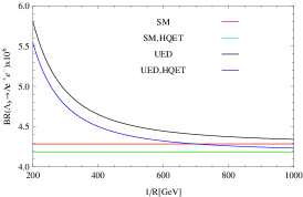
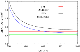
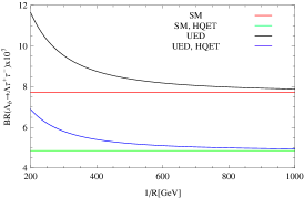
Figure 1: The dependence of branching ratios on compactification factor, $1/R$.

From this figure, we deduce the following results:

• There is considerable discrepancy between the predictions of the ACD and SM models for low values of the compactification factor, $1/R$. As $1/R$ increases, this difference tends to diminish so that for higher values of $1/R$ ($1/R\simeq 1000~{}GeV$), the predictions of ACD become very close to the results of SM . Such discrepancy at low values of $1/R$ can be considered as a signal for the existence of extra dimensions.

• As it is expected, an increase in the lepton mass ends up in a decrease in the branching ratio.

• The order of magnitude of the branching ratio shows a possibility to study such channels at the LHC.

• The $\Lambda_{b}\rightarrow\Lambda\ell^{+}\ell^{-}$ transition is more probable, specially for $\tau$ case, in full theory in comparison with HQET.

3.2 Forward Backward Asymmetry

The lepton forward-backward asymmetry is one of the promising tools in looking for new physics beyond the SM such as extra dimensions. This asymmetry is defined as:

$${\cal A}_{FB}=\frac{N_{f}-N_{b}}{N_{f}+N_{b}}$$ (3.41)

where $N_{f}$ is the number of events that particle is moving ”forward” with respect to any chosen direction, while $N_{b}$ is the number of events for particle motion in ”backward” direction. The forward–backward asymmetry ${\cal A}_{FB}(\hat{s},1/R)$ is defined in terms of the differential decay rate as:

$${\cal A}_{FB}(\hat{s},1/R)=\frac{\displaystyle{\int_{0}^{1}\frac{d\Gamma}{d\hat{s}dz}}(z,\hat{s},1/R)\,dz-\displaystyle{\int_{-1}^{0}\frac{d\Gamma}{d\hat{s}dz}}(z,\hat{s},1/R)\,dz}{\displaystyle{\int_{0}^{1}\frac{d\Gamma}{d\hat{s}dz}}(z,\hat{s},1/R)\,dz+\displaystyle{\int_{-1}^{0}\frac{d\Gamma}{d\hat{s}dz}}(z,\hat{s},1/R)\,dz}~{}.$$ (3.42)

We depict the dependence of ${\cal A}_{FB}(\hat{s},1/R)$ asymmetry on $1/R$ for different leptons and at a fixed value of $\hat{s}=0.5$ common for allowed physical regions of all leptons in Fig. 2.

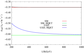
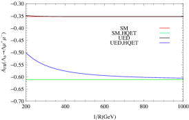
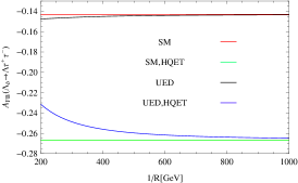
Figure 2: The dependence of ${\cal A}_{FB}(\hat{s},1/R)$ asymmetry on compactification factor, $1/R$ for different leptons at $\hat{s}=0.5$.

A quick glance at these figures leads to the following results:

• The ${\cal A}_{FB}$ is approximately the same for $e$ and $\mu$ and about 2-2.5 times greater than that of $\tau$ case.

• As far as HQET is considered, there is considerable discrepancy between the predictions of the ACD and SM models for low values of $1/R$. As $1/R$ increases, this difference starts to diminish and at $1/R\simeq 1000~{}GeV$, the two models have approximately the same results. In full theory, two models have approximately the same predictions for all leptons and all $1/R$ values.

• For all leptons, the forward-backward asymmetries show considerable differences between the full theory and HQET predictions.

3.3 $\Lambda$ Baryon Polarizations

The definitions for polarizations of $\Lambda$ baryon in $\Lambda_{b}\rightarrow\Lambda\ell^{+}\ell^{-}$ channel are given in [30]. Using those definitions, the $1/R$-dependent normal ($P_{N}$), transversal ($P_{T}$) and longitudinal ($P_{L}$) polarizations of the $\Lambda$ baryon in the massive lepton case are found as (for the general model independent case see [26, 31]):

$$P_{N}(\hat{s},1/R)\!\!\! = \!\!\!\frac{8\pi m_{\Lambda_{b}}^{3}v\sqrt{\hat{s}}}{\Delta(\hat{s},1/R)}\Bigg{\{}-2m_{\Lambda_{b}}(1-r+\hat{s})\sqrt{r}\,\mbox{\rm Re}[A_{1}^{\ast}D_{1}+B_{1}^{\ast}E_{1}]$$ (3.43)

$$+ \!\!\!m_{\Lambda_{b}}(1-\sqrt{r})[(1+\sqrt{r})^{2}-\hat{s}]\,\Big{(}m_{\ell}\mbox{\rm Re}[(A_{2}-B_{2})^{\ast}F_{1}]\Big{)}$$

$$+ \!\!\!m_{\ell}[(1+\sqrt{r})^{2}-\hat{s}]\,\mbox{\rm Re}[A_{1}^{\ast}F_{1}]$$

$$+ \!\!\!4m_{\Lambda_{b}}^{2}\hat{s}\sqrt{r}\,\mbox{\rm Re}[A_{1}^{\ast}E_{2}+A_{2}^{\ast}E_{1}+B_{1}^{\ast}D_{2}+B_{2}^{\ast}D_{1}]$$

$$- \!\!\!2m_{\Lambda_{b}}^{3}\hat{s}\sqrt{r}(1-r+\hat{s})\,\mbox{\rm Re}[A_{2}^{\ast}D_{2}+B_{2}^{\ast}E_{2}^{\ast}]$$

$$+ \!\!\!2m_{\Lambda_{b}}(1-r-\hat{s})\,\Big{(}\mbox{\rm Re}[A_{1}^{\ast}E_{1}+B_{1}^{\ast}D_{1}]+m_{\Lambda_{b}}^{2}\hat{s}\mbox{\rm Re}[A_{2}^{\ast}E_{2}+B_{2}^{\ast}D_{2}]\Big{)}$$

$$- \!\!\!m_{\Lambda_{b}}^{2}[(1-r)^{2}-\hat{s}^{2}]\,\mbox{\rm Re}[A_{1}^{\ast}D_{2}+A_{2}^{\ast}D_{1}+B_{1}^{\ast}E_{2}+B_{2}^{\ast}E_{1}]$$

$$- \!\!\!m_{\ell}[(1+\sqrt{r})^{2}-\hat{s}]\,\mbox{\rm Re}[B_{1}^{\ast}F_{1}]\Bigg{\}}~{},$$

$$P_{T}(\hat{s},1/R)=-\frac{8\pi m_{\Lambda_{b}}^{3}v\sqrt{\hat{s}\lambda}}{\Delta(\hat{s},1/R)}\Bigg{\{}m_{\ell}\Big{(}\mbox{\rm Im}[(A_{1}+B_{1})^{\ast}F_{1}]\Big{)}$$ (3.44)

$$- \!\!\!m_{\ell}m_{\Lambda_{b}}\Big{[}(1+\sqrt{r})\,\mbox{\rm Im}[(A_{2}+B_{2})^{\ast}F_{1}]\Big{]}$$

$$+ \!\!\!m_{\Lambda_{b}}^{2}(1-r+\hat{s})\Big{(}\mbox{\rm Im}[A_{2}^{\ast}D_{1}-A_{1}^{\ast}D_{2}]-\mbox{\rm Im}[B_{2}^{\ast}E_{1}-B_{1}^{\ast}E_{2}]\Big{)}$$

$$+ \!\!\!2m_{\Lambda_{b}}\Big{(}\mbox{\rm Im}[A_{1}^{\ast}E_{1}-B_{1}^{\ast}D_{1}]-m_{\Lambda_{b}}^{2}\hat{s}\,\mbox{\rm Im}[A_{2}^{\ast}E_{2}-B_{2}^{\ast}D_{2}]\Big{)}\Bigg{\}}~{},$$

$$P_{L}(\hat{s},1/R)\!\!\! = \!\!\!\frac{16m_{\Lambda_{b}}^{2}\sqrt{\lambda}}{\Delta(\hat{s},1/R)}\Bigg{\{}8m_{\ell}^{2}m_{\Lambda_{b}}\,\Big{(}\mbox{\rm Re}[D_{1}^{\ast}E_{3}-D_{3}^{\ast}E_{1}]+\sqrt{r}\mbox{\rm Re}[D_{1}^{\ast}D_{3}-E_{1}^{\ast}E_{3})]\Big{)}$$ (3.45)

$$+ \!\!\!2m_{\ell}m_{\Lambda_{b}}\,(1+\sqrt{r})\mbox{\rm Re}[(D_{1}-E_{1})^{\ast}F_{2}]$$

$$- \!\!\!2m_{\ell}m_{\Lambda_{b}}^{2}\hat{s}\,\Big{\{}\mbox{\rm Re}[(D_{3}-E_{3})^{\ast}F_{2}]+2m_{\ell}(\left|D_{3}\right|^{2}-\left|E_{3}\right|^{2})\Big{\}}$$

$$- \!\!\!4m_{\Lambda_{b}}(2m_{\ell}^{2}+m_{\Lambda_{b}}^{2}\hat{s})\,\mbox{\rm Re}[A_{1}^{\ast}B_{2}-A_{2}^{\ast}B_{1}]$$

$$- \!\!\!\frac{4}{3}m_{\Lambda_{b}}^{3}\hat{s}v^{2}\,\Big{(}3\mbox{\rm Re}[D_{1}^{\ast}E_{2}-D_{2}^{\ast}E_{1}]+\sqrt{r}\mbox{\rm Re}[D_{1}^{\ast}D_{2}-E_{1}^{\ast}E_{2}]\Big{)}$$

$$- \!\!\!\frac{4}{3}m_{\Lambda_{b}}\sqrt{r}(6m_{\ell}^{2}+m_{\Lambda_{b}}^{2}\hat{s}v^{2})\,\mbox{\rm Re}[A_{1}^{\ast}A_{2}-B_{1}^{\ast}B_{2}]$$

$$+ \!\!\!\frac{1}{3}\Big{\{}3[4m_{\ell}^{2}+m_{\Lambda_{b}}^{2}(1-r+\hat{s})](\left|A_{1}\right|^{2}-\left|B_{1}\right|^{2})-3[4m_{\ell}^{2}-m_{\Lambda_{b}}^{2}(1-r+\hat{s})]$$

$$\times \!\!\!(\left|D_{1}\right|^{2}-\left|E_{1}\right|^{2})-m_{\Lambda_{b}}^{2}(1-r-\hat{s})v^{2}(\left|A_{1}\right|^{2}-\left|B_{1}\right|^{2}+\left|D_{1}\right|^{2}-\left|E_{1}\right|^{2})\Big{\}}$$

$$- \!\!\!\frac{1}{3}m_{\Lambda_{b}}^{2}\{12m_{\ell}^{2}(1-r)+m_{\Lambda_{b}}^{2}\hat{s}[3(1-r+\hat{s})+v^{2}(1-r-\hat{s})]\}(\left|A_{2}\right|^{2}-\left|B_{2}\right|^{2})$$

$$- \!\!\!\frac{2}{3}m_{\Lambda_{b}}^{4}\hat{s}(2-2r+\hat{s})v^{2}\,(\left|D_{2}\right|^{2}-\left|E_{2}\right|^{2})\Bigg{\}}~{},$$

where,

$$\Delta(\hat{s},1/R)\!\!\! = \!\!\!{{\cal T}_{0}(\hat{s},1/R)+\frac{1}{3}{\cal T}_{2}(\hat{s},1/R)}.$$ (3.46)

For instance, we show the dependence of the $P_{N}$ and $P_{T}$ polarizations of the $\Lambda$ baryon on compactification factor at a fixed value of $\hat{s}=0.5$ in Figs. 3 and 4 , respectively. From these figures, we infer the following information:

• In the case of $P_{N}$ and all leptons, we observe a (25-35)% HQET violations. This violation is very small for the transverse polarization of the $\Lambda$.

• The UED predictions deviate considerably from the SM results in the case of $P_{T}$ and small values of the compactification factor. This deviation is small for the $P_{N}$ compared to the $P_{T}$. In the case of $\tau$ and HQET, two models have approximately the same predictions for the normal polarization.

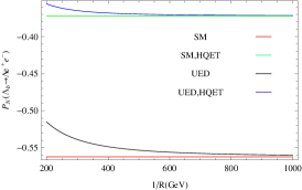
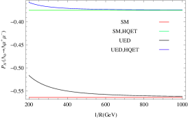
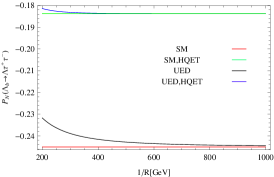
Figure 3: The dependence of $P_{N}(\hat{s},1/R)$ on compactification factor, $1/R$ for different leptons at $\hat{s}=0.5$.

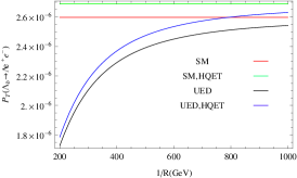
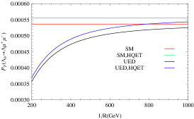
Figure 4: The dependence of $P_{T}(\hat{s},1/R)$ on compactification factor, $1/R$ for different leptons at $\hat{s}=0.5$.

3.4 Double Lepton Polarization Asymmetries

The double lepton polarization asymmetries related to the $\Lambda_{b}\rightarrow\Lambda\ell^{+}\ell^{-}$ transition are defined in [32] for general model independent form of the effective Hamiltonian. In our case, in the rest frame of $\ell^{\pm}$, the $1/R$-dependent double longitudinal, transverse and normal asymmetries are obtained as (see also [33, 34]):

$$P_{LN}(\hat{s},1/R)\!\!\! = \!\!\!\frac{16\pi m_{\Lambda_{b}}^{4}\hat{m}_{\ell}\sqrt{\lambda}}{\Delta(\hat{s},1/R)\sqrt{\hat{s}}}\mbox{\rm Im}\Bigg{\{}(1-r)(A_{1}^{\ast}D_{1}+B_{1}^{\ast}E_{1})+m_{\Lambda_{b}}\hat{s}(A_{1}^{\ast}E_{3}-A_{2}^{\ast}E_{1}+B_{1}^{\ast}D_{3}-B_{2}^{\ast}D_{1})$$ (3.47)

$$+ \!\!\!m_{\Lambda_{b}}\sqrt{r}\hat{s}(A_{1}^{\ast}D_{3}+A_{2}^{\ast}D_{1}+B_{1}^{\ast}E_{3}+B_{2}^{\ast}E_{1})-m_{\Lambda_{b}}^{2}\hat{s}^{2}\Big{(}B_{2}^{\ast}E_{3}+A_{2}^{\ast}D_{3}\Big{)}\Bigg{\}},$$

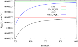
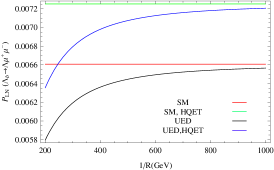
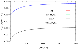
Figure 5: The dependence of $P_{LN}(\hat{s},1/R)$ on compactification factor, $1/R$ for different leptons at $\hat{s}=0.5$.

$$P_{NL}(\hat{s},1/R)\!\!\! = \!\!\!-\frac{16\pi m_{\Lambda_{b}}^{4}\hat{m}_{\ell}\sqrt{\lambda}}{\Delta\sqrt{\hat{s}}}\mbox{\rm Im}\Bigg{\{}(1-\hat{r}_{\Lambda})(A_{1}^{\ast}D_{1}+B_{1}^{\ast}E_{1})+m_{\Lambda_{b}}\hat{s}(A_{1}^{\ast}E_{3}-A_{2}^{\ast}E_{1}+B_{1}^{\ast}D_{3}-B_{2}^{\ast}D_{1})$$ (3.48)

$$- \!\!\!m_{\Lambda_{b}}\sqrt{\hat{r}_{\Lambda}}\hat{s}(A_{1}^{\ast}D_{3}+A_{2}^{\ast}D_{1}+B_{1}^{\ast}E_{3}+B_{2}^{\ast}E_{1})-m_{\Lambda_{b}}^{2}\hat{s}^{2}\Big{(}B_{2}^{\ast}E_{3}+A_{2}^{\ast}D_{3}\Big{)}\Bigg{\}},$$

$$P_{LT}(\hat{s},1/R)\!\!\! = \!\!\!\frac{16\pi m_{\Lambda_{b}}^{4}\hat{m}_{\ell}\sqrt{\lambda}v}{\Delta(\hat{s},1/R)\sqrt{\hat{s}}}\mbox{\rm Re}\Bigg{\{}(1-r)\Big{(}\left|D_{1}\right|^{2}+\left|E_{1}\right|^{2}\Big{)}-\hat{s}\Big{(}A_{1}D_{1}^{\ast}-B_{1}E_{1}^{\ast}\Big{)}$$ (3.49)

$$- \!\!\!m_{\Lambda_{b}}\hat{s}\Big{[}B_{1}D_{2}^{\ast}+(A_{2}+D_{2}-D_{3})E_{1}^{\ast}-A_{1}E_{2}^{\ast}-(B_{2}-E_{2}+E_{3})D_{1}^{\ast}\Big{]}$$

$$+ \!\!\!m_{\Lambda_{b}}\sqrt{r}\hat{s}\Big{[}A_{1}D_{2}^{\ast}+(A_{2}+D_{2}+D_{3})D_{1}^{\ast}-B_{1}E_{2}^{\ast}-(B_{2}-E_{2}-E_{3})E_{1}^{\ast}\Big{]}$$

$$+ \!\!\!m_{\Lambda_{b}}^{2}\hat{s}(1-r)(A_{2}D_{2}^{\ast}-B_{2}E_{2}^{\ast})-m_{\Lambda_{b}}^{2}\hat{s}^{2}(D_{2}D_{3}^{\ast}+E_{2}E_{3}^{\ast})\Bigg{\}},$$

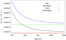
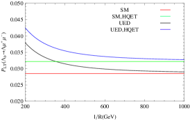
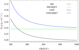
Figure 6: The dependence of $P_{LT}(\hat{s},1/R)$ on compactification factor, $1/R$ for different leptons at $\hat{s}=0.5$.

$$P_{TL}(\hat{s},1/R)\!\!\! = \!\!\!\frac{16\pi m_{\Lambda_{b}}^{4}\hat{m}_{\ell}\sqrt{\lambda}v}{\Delta\sqrt{\hat{s}}}\mbox{\rm Re}\Bigg{\{}(1-\hat{r}_{\Lambda})\Big{(}\left|D_{1}\right|^{2}+\left|E_{1}\right|^{2}\Big{)}+\hat{s}\Big{(}A_{1}D_{1}^{\ast}-B_{1}E_{1}^{\ast}\Big{)}$$ (3.50)

$$+ \!\!\!m_{\Lambda_{b}}\hat{s}\Big{[}B_{1}D_{2}^{\ast}+(A_{2}-D_{2}+D_{3})E_{1}^{\ast}-A_{1}E_{2}^{\ast}-(B_{2}+E_{2}-E_{3})D_{1}^{\ast}\Big{]}$$

$$- \!\!\!m_{\Lambda_{b}}\sqrt{\hat{r}_{\Lambda}}\hat{s}\Big{[}A_{1}D_{2}^{\ast}+(A_{2}-D_{2}-D_{3})D_{1}^{\ast}-B_{1}E_{2}^{\ast}-(B_{2}+E_{2}+E_{3})E_{1}^{\ast}\Big{]}$$

$$- \!\!\!m_{\Lambda_{b}}^{2}\hat{s}(1-\hat{r}_{\Lambda})(A_{2}D_{2}^{\ast}-B_{2}E_{2}^{\ast})-m_{\Lambda_{b}}^{2}\hat{s}^{2}(D_{2}D_{3}^{\ast}+E_{2}E_{3}^{\ast})\Bigg{\}},$$

$$P_{LL}(\hat{s},1/R)\!\!\! = \!\!\!\frac{16m_{\Lambda_{b}}^{4}}{3\Delta(\hat{s},1/R)}\mbox{\rm Re}\Bigg{\{}$$ (3.51)

$$- \!\!\!6m_{\Lambda_{b}}\sqrt{r}(1-r+\hat{s})\Big{[}\hat{s}(1+v^{2})(A_{1}A_{2}^{\ast}+B_{1}B_{2}^{\ast})-4\hat{m}_{\ell}^{2}(D_{1}D_{3}^{\ast}+E_{1}E_{3}^{\ast})\Big{]}$$

$$+ \!\!\!6m_{\Lambda_{b}}(1-r-\hat{s})\Big{[}\hat{s}(1+v^{2})(A_{1}B_{2}^{\ast}+A_{2}B_{1}^{\ast})+4\hat{m}_{\ell}^{2}(D_{1}E_{3}^{\ast}+D_{3}E_{1}^{\ast})\Big{]}$$

$$+ \!\!\!12\sqrt{r}\hat{s}(1+v^{2})\Big{(}A_{1}B_{1}^{\ast}+D_{1}E_{1}^{\ast}+m_{\Lambda_{b}}^{2}\hat{s}A_{2}B_{2}^{\ast}\Big{)}$$

$$+ \!\!\!12m_{\Lambda_{b}}^{2}\hat{m}_{\ell}^{2}\hat{s}(1+r-\hat{s})\left(\left|D_{3}\right|^{2}+\left|E_{3}^{\ast}\right|^{2}\right)$$

$$- \!\!\!(1+v^{2})\Big{[}1+r^{2}-r(2-\hat{s})+\hat{s}(1-2\hat{s})\Big{]}\Big{(}\left|A_{1}\right|^{2}+\left|B_{1}\right|^{2}\Big{)}$$

$$- \!\!\!\Big{[}(5v^{2}-3)(1-r)^{2}+4\hat{m}_{\ell}^{2}(1+r)+2\hat{s}(1+8\hat{m}_{\ell}^{2}+r)-4\hat{s}^{2}\Big{]}\Big{(}\left|D_{1}\right|^{2}+\left|E_{1}\right|^{2}\Big{)}$$

$$- \!\!\!m_{\Lambda_{b}}^{2}(1+v^{2})\hat{s}\Big{[}2+2r^{2}-\hat{s}(1+\hat{s})-r(4+\hat{s})\Big{]}\big{(}\left|A_{2}\right|^{2}+\left|B_{2}\right|^{2}\Big{)}$$

$$- \!\!\!2m_{\Lambda_{b}}^{2}\hat{s}v^{2}\Big{[}2(1+r^{2})-\hat{s}(1+\hat{s})-r(4+\hat{s})\Big{]}\Big{(}\left|D_{2}\right|^{2}+\left|E_{2}\right|^{2}\Big{)}$$

$$+ \!\!\!12m_{\Lambda_{b}}\hat{s}(1-r-\hat{s})v^{2}\Big{(}D_{1}E_{2}^{\ast}+D_{2}E_{1}^{\ast}\Big{)}$$

$$- \!\!\!12m_{\Lambda_{b}}\sqrt{r}\hat{s}(1-r+\hat{s})v^{2}\Big{(}D_{1}D_{2}^{\ast}+E_{1}E_{2}^{\ast}\Big{)}$$

$$+ \!\!\!24m_{\Lambda_{b}}^{2}\sqrt{r}\hat{s}\Big{(}\hat{s}v^{2}D_{2}E_{2}^{\ast}+2\hat{m}_{\ell}^{2}D_{3}E_{3}^{\ast}\Big{)}\Bigg{\}},$$

$$P_{NT}(\hat{s},1/R)\!\!\! = \!\!\!\frac{64m_{\Lambda_{b}}^{4}\lambda v}{3\Delta(\hat{s},1/R)}\mbox{\rm Im}\Bigg{\{}(A_{1}D_{1}^{\ast}+B_{1}E_{1}^{\ast})+m_{\Lambda_{b}}^{2}\hat{s}(A_{2}^{\ast}D_{2}+B_{2}^{\ast}E_{2})\Bigg{\}},$$ (3.52)

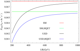
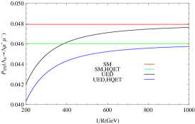
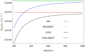
Figure 7: The dependence of $P_{TN}(\hat{s},1/R)$ on compactification factor, $1/R$ for different leptons at $\hat{s}=0.5$.

$$P_{TN}(\hat{s},1/R)\!\!\! = \!\!\!-\frac{64m_{\Lambda_{b}}^{4}\lambda v}{3\Delta}\mbox{\rm Im}\Bigg{\{}(A_{1}D_{1}^{\ast}+B_{1}E_{1}^{\ast})+m_{\Lambda_{b}}^{2}\hat{s}(A_{2}^{\ast}D_{2}+B_{2}^{\ast}E_{2})\Bigg{\}},$$ (3.53)

$$P_{NN}(\hat{s},1/R)\!\!\! = \!\!\!\frac{32m_{\Lambda_{b}}^{4}}{3\hat{s}\Delta(\hat{s},1/R)}\mbox{\rm Re}\Bigg{\{}24\hat{m}_{\ell}^{2}\sqrt{r}\hat{s}(A_{1}B_{1}^{\ast}+D_{1}E_{1}^{\ast})$$ (3.54)

$$- \!\!\!12m_{\Lambda_{b}}\hat{m}_{\ell}^{2}\sqrt{r}\hat{s}(1-r+\hat{s})(A_{1}A_{2}^{\ast}+B_{1}B_{2}^{\ast})$$

$$+ \!\!\!6m_{\Lambda_{b}}\hat{m}_{\ell}^{2}\hat{s}\Big{[}m_{\Lambda_{b}}\hat{s}(1+r-\hat{s})\Big{(}\left|D_{3}\right|^{2}+\left|E_{3}\right|^{2}\Big{)}+2\sqrt{r}(1-r+\hat{s})(D_{1}D_{3}^{\ast}+E_{1}E_{3}^{\ast})\Big{]}$$

$$+ \!\!\!12m_{\Lambda_{b}}\hat{m}_{\ell}^{2}\hat{s}(1-r-\hat{s})(A_{1}B_{2}^{\ast}+A_{2}B_{1}^{\ast}+D_{1}E_{3}^{\ast}+D_{3}E_{1}^{\ast})$$

$$- \!\!\![\lambda\hat{s}+2\hat{m}_{\ell}^{2}(1+r^{2}-2r+r\hat{s}+\hat{s}-2\hat{s}^{2})]\Big{(}\left|A_{1}\right|^{2}+\left|B_{1}\right|^{2}-\left|D_{1}\right|^{2}-\left|E_{1}\right|^{2}\Big{)}$$

$$+ \!\!\!24m_{\Lambda_{b}}^{2}\hat{m}_{\ell}^{2}\sqrt{r}\hat{s}^{2}(A_{2}B_{2}^{\ast}+D_{3}E_{3}^{\ast})-m_{\Lambda_{b}}^{2}\lambda\hat{s}^{2}v^{2}\Big{(}\left|D_{2}\right|^{2}+\left|E_{2}\right|^{2}\Big{)}$$

$$+ \!\!\!m_{\Lambda_{b}}^{2}\hat{s}\{\lambda\hat{s}-2\hat{m}_{\ell}^{2}[2(1+r^{2})-\hat{s}(1+\hat{s})-r(4+\hat{s})]\}\Big{(}\left|A_{2}\right|^{2}+\left|B_{2}\right|^{2}\Big{)}\Bigg{\}},$$

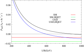
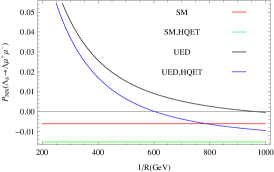
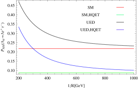
Figure 8: The dependence of $P_{NN}(\hat{s},1/R)$ on compactification factor, $1/R$ for different leptons at $\hat{s}=0.5$.

$$P_{TT}(\hat{s},1/R)\!\!\! = \!\!\!\frac{32m_{\Lambda_{b}}^{4}}{3\hat{s}\Delta(\hat{s},1/R)}\mbox{\rm Re}\Bigg{\{}-24\hat{m}_{\ell}^{2}\sqrt{r}\hat{s}(A_{1}B_{1}^{\ast}+D_{1}E_{1}^{\ast})$$ (3.55)

$$- \!\!\!12m_{\Lambda_{b}}\hat{m}_{\ell}^{2}\sqrt{r}\hat{s}(1-r+\hat{s})(D_{1}D_{3}^{\ast}+E_{1}E_{3}^{\ast})-24m_{\Lambda_{b}}^{2}\hat{m}_{\ell}^{2}\sqrt{r}\hat{s}^{2}(A_{2}B_{2}^{\ast}+D_{3}E_{3}^{\ast})$$

$$- \!\!\!6m_{\Lambda_{b}}\hat{m}_{\ell}^{2}\hat{s}\Big{[}m_{\Lambda_{b}}\hat{s}(1+r-\hat{s})\Big{(}\left|D_{3}\right|^{2}+\left|E_{3}\right|^{2}\Big{)}-2\sqrt{r}(1-r+\hat{s})(A_{1}A_{2}^{\ast}+B_{1}B_{2}^{\ast})\Big{]}$$

$$- \!\!\!12m_{\Lambda_{b}}\hat{m}_{\ell}^{2}\hat{s}(1-r-\hat{s})(A_{1}B_{2}^{\ast}+A_{2}B_{1}^{\ast}+D_{1}E_{3}^{\ast}+D_{3}E_{1}^{\ast})$$

$$- \!\!\![\lambda\hat{s}-2\hat{m}_{\ell}^{2}(1+r^{2}-2r+r\hat{s}+\hat{s}-2\hat{s}^{2})]\Big{(}\left|A_{1}\right|^{2}+\left|B_{1}\right|^{2}\Big{)}$$

$$+ \!\!\!m_{\Lambda_{b}}^{2}\hat{s}\{\lambda\hat{s}+\hat{m}_{\ell}^{2}[4(1-r)^{2}-2\hat{s}(1+r)-2\hat{s}^{2}]\}\Big{(}\left|A_{2}\right|^{2}+\left|B_{2}\right|^{2}\Big{)}$$

$$+ \!\!\!\{\lambda\hat{s}-2\hat{m}_{\ell}^{2}[5(1-r)^{2}-7\hat{s}(1+r)+2\hat{s}^{2}]\}\Big{(}\left|D_{1}\right|^{2}+\left|E_{1}\right|^{2}\Big{)}$$

$$- \!\!\!m_{\Lambda_{b}}^{2}\lambda\hat{s}^{2}v^{2}\Big{(}\left|D_{2}\right|^{2}+\left|E_{2}\right|^{2}\Big{)}\Bigg{\}},$$

where, $\hat{m}_{l}=\frac{m_{l}}{m_{\Lambda_{b}}}$. As examples, we depict the $1/R$ dependence of some double lepton polarization asymmetries at a fixed value of $\hat{s}=0.5$ in Figs. 5-9. From these figures, we obtain the following conclusions:

• In all cases, there are substantial differences between predictions of the ACD and SM models in low values of the compactification parameter, $1/R$.

• We observe overall considerable differences between predictions of the full QCD and HQET for double lepton polarization asymmetries.

• All polarization asymmetries have the same sign for all leptons except the $P_{TT}$, which predicts a different sign for $\tau$ compared to the $e$ and $\mu$. In the case of $e$ and $\mu$ and HQET, the $P_{NN}$ changes its sign around $1/R=600~{}GeV$. In $P_{NN}$, the full QCD predicts different sign for the ACD and SM models for these two leptons although the SM results are very small.

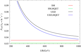
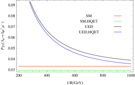
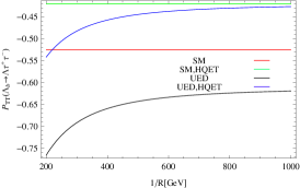
Figure 9: The dependence of $P_{TT}(\hat{s},1/R)$ on compactification factor, $1/R$ for different leptons at $\hat{s}=0.5$.

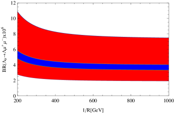
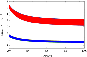
Figure 10: The dependence of branching ratios on compactification factor, $1/R$, when errors of the form factors are considered. The red and blue bands belong to the full QCD and HQET, respectively.

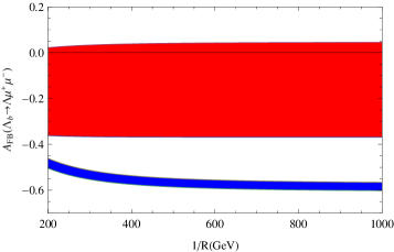
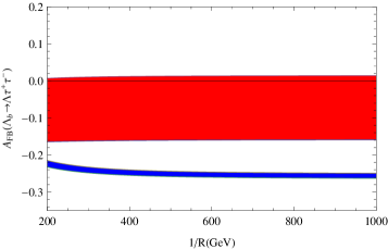
Figure 11: The same as Figure 10, but for ${\cal A}_{FB}$ asymmetries.

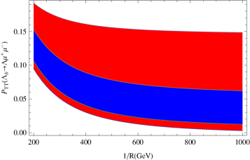
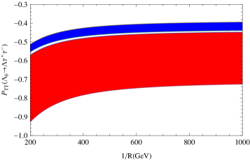
Figure 12: The same as Figure 10, but for $P_{TT}$ polarization.

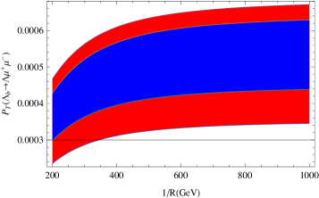
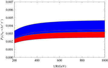
Figure 13: The same as Figure 10, but for $P_{T}$ polarization.

At the end of this section, we would like to compare the full theory and HQET predictions on some observables considering the errors of form factors. In Figs. 1-9, we compared the results of two theories when the central values of the form factors are used. Now, in Figs. 10-13, we depict the dependence of some considered observables on compactification factor, $1/R$ at a fixed value of $\hat{s}=0.5$ and compare predictions of two theories when the uncertainties of the form factors are taken into account. The red bands in these figures belong to the full theory and they are obtained considering the errors of the form factors presented in [11], while the blue bands correspond to the HQET and they are obtained using the errors of the form factors presented in [12]. Here, we should stress that the reported errors of the form factors in HQET are small comparing those presented in full QCD, hence the HQET bands are narrow comparing to the full theory bands. From figure 10, we see a significant difference between the predictions of two theories for $\tau$ case, while in the $\mu$ case, the HQET band lies inside the full QCD region. In the case of ${\cal A}_{FB}$ in figure 11, we see also considerable difference between delimited regions of full and HQET theories for both leptons. In the case of $\mu$ and $P_{TT}$ and $P_{T}$ polarizations (see figures 12 and 13), predictions of the HQET lie inside the full theory bands, but in the case of $\tau$ and $P_{TT}$, the band of HQET is out of the band of full theory but very close to it. In $P_{T}$ polarization and $\tau$, two bands partly coincide with each other.

4 Conclusion

We analyzed the branching ratio, forward-backward asymmetry, double lepton polarization asymmetries and polarization of the $\Lambda$ baryon for the channel, $\Lambda_{b}\rightarrow\Lambda\ell^{+}\ell^{-}$ in the universal extra dimension scenario using the form factors obtained from both full QCD and HQET. For each case, we compared the obtained results with predictions of the SM. In lower values of the compactification factor, we see considerable discrepancy between the UED and SM models. However, when $1/R$ grows, the results of UED tend to diminish and at $1/R=1000~{}GeV$, two models have approximately the same predictions. The order of magnitude for branching ratios shows a possibility to study this channel at LHCb. The obtained results for the branching fractions show also that this transition is more probable in full QCD compared to the HQET. For other observables, we see also overall substantial differences between predictions of the full theory and HQET specially when the central values of the form factors from both theories are used. Any measurements on the considered physical quantities in this manuscript and their comparison with our predictions, can give useful information about existing of extra dimensions.

References

- [1] I. Antoniadis, Phys. Lett. B 246, 377 (1990).
- [2] I. Antoniadis, N. Arkani-Hamed, S. Dimopoulos and G. Dvali, Phys. Lett. B 439, 257 (1998).
- [3] N. Arkani-Hamed, S. Dimopoulos and G. Dvali, Phys. Lett. B 429, 263 (1998); Phys. Rev. D 59, 086004 (1999).
- [4] T. Appelquist, H. C. Cheng and B. A. Dobrescu, Phys. Rev. D 64, 035002 (2001).
- [5] A. J. Buras, M. Spranger and A. Weiler, Nucl. Phys. B 660, 225 (2003).
- [6] A. J. Buras, A. Poschenrieder, M. Spranger Nucl. Phys. B D 678, 455 (2004).
- [7] P. Colangelo, F. De Fazio, R. Ferrandes, T. N. Pham, Phys. Rev. D7 3 (2006) 115006.
- [8] G. Buchalla, G. Hiller and G. Isidori, Phys. Rev. D 63 (2000) 014015.
- [9] C. Bird, P. Jackson, R. Kowalewski, M. Pospelov, Phys. Rev. Lett. 93 (2004) 201803.
- [10] T. Appelquist and H. U. Yee, Phys. Rev. D 67 (2003) 055002.
- [11] T. M. Aliev, K. Azizi, M. Savci, Phys. Rev. D, 81, 056006, (2010).
- [12] C. S. Huang, H. G. Yan, Phys. Rev. D 59, 114022 (1999).
- [13] P. Colangelo, F. De Fazio, R. Ferrandes, T. N. Pham, Phys. Rev. D 77, 055019 (2008).
- [14] T. M. Aliev, M. Savcı, Eur. Phys. J. C 50, 91 (2007).
- [15] Yu-Ming Wang, M. Jamil Aslam, Cai-Dian Lu, Eur. Phys. J. C 59, 847 (2009).
- [16] M.V. Carlucci, P. Colangelo, F. De Fazio, Phys. Rev. D 80, 055023 (2009).
- [17] Ishtiaq Ahmed, M. Ali Paracha, M. Jamil Aslam, Eur. Phys. J. C 54, 591 (2008).
- [18] Asif Saddique, M. Jamil Aslam, Cai-Dian Lu, Eur. Phys. J. C 56, 267 (2008).
- [19] V. Bashiry, K. Zeynali, Phys. Rev. D 79, 033006 (2009).
- [20] A. Buras, M. Misiak, M. Münz and S. Pokorski, Nucl. Phys. B 424, 374 (1994).
- [21] M. Misiak, Nucl. Phys. B 393, 23 (1993); Erratum ibid B 439, 161 (1995).
- [22] B. Buras, M. Münz, Phys. Rev. D 52, 186 (1995).
- [23] T. M. Aliev, A. Ozpineci, M. Savci, Phys. Rev. D 65 (2002) 115002.
- [24] T. Mannel, W. Roberts and Z. Ryzak, Nucl. Phys. B355 (1991) 38.
- [25] C. H. Chen, C. Q. Geng, Phys. Rev. D 63 (2001) 054005; Phys. Rev. D 63 (2001) 114024; Phys. Rev. D 64 (2001) 074001.
- [26] T. M. Aliev, A. Ozpineci, M. Savci, C. Yuce , Phys. Lett. B 542 (2002) 229.
- [27] T. M. Aliev, A. Ozpineci, M. Savci, Nucl .Phys. B 649 (2003) 168.
- [28] A. K. Giri, R. Mohanta, Eur. Phys. J. C 45, 151 (2006).
- [29] C. Amsler et al. [Particle Data Group], Phys. Lett. B 667, 1 (2008).
- [30] T. M. Aliev, A. Özpineci, M. Savcı, Phys. Rev. D 67, 035007 (2003).
- [31] T. M. Aliev, A. Ozpineci, M. Savci, arXiv:hep-ph/0301019.
- [32] T. M. Aliev, V. Bashiry, M. Savci, Eur. Phys. J. C 38 (2004) 283.
- [33] T. M. Aliev, M. Savci, B. B. Sirvanli, Eur. Phys.J. C 52, 375 (2007).
- [34] W. Bensalem, D. London, N. Sinha and R. Sinha, Phys. Rev. D 67, 034007 (2003).