The Tayler instability of toroidal magnetic fields in a columnar gallium experiment

Abstract

The nonaxisymmetric Tayler instability of toroidal magnetic fields due to axial electric currents is studied for conducting incompressible fluids between two coaxial cylinders without endplates. The inner cylinder is considered as so thin that even the limit of $R_{\rm in}\to 0$ can be computed. The magnetic Prandtl number is varied over many orders of magnitudes but the azimuthal mode number of the perturbations is fixed to $m=1$. In the linear approximation the critical magnetic field amplitudes and the growth rates of the instability are determined for both resting and rotating cylinders. Without rotation the critical Hartmann numbers do not depend on the magnetic Prandtl number but this is not true for the growth rates. For given product of viscosity and magnetic diffusivity the growth rates for small and large magnetic Prandtl number are much smaller than those for $\rm Pm=1$. For gallium under the influence of a magnetic field at the outer cylinder of 1 kG the resulting growth time is 5 s. The minimum electric current through a container of 10 cm diameter to excite the kink-type instability is 3.20 kA. For a rotating container both the critical magnetic field and the related growth times are larger than for the resting column.

1 Motivation

A known instability of toroidal fields is the current-driven (‘kink-type’) Tayler instability (TI) which is basically nonaxisymmetric (Tayler 1957; Vandakurov 1972; Tayler 1973; Acheson 1978). The toroidal field becomes unstable against nonaxisymmetric perturbations for a sufficiently large magnetic field amplitude depending on the radial profile of the field. A global rigid rotation of the system stabilizes the TI, i.e. much higher field amplitudes can be kept stable. For the rapidly rotating regime ${\it\Omega}>{\it\Omega}_{\rm A}$ (with ${\it\Omega}_{\rm A}$ is the Alfvén frequency of the toroidal field) the stability becomes complete, i.e. all possible modes in incompressible fluids of uniform density are stable (Pitts & Tayler 1985). We shall demonstrate in the present paper how this instability and its stabilization by rigid rotation can experimentally be realized with fluid conductors like sodium or gallium. There is so far no empirical or observational proof of the existence of the TI (Maeder & Meynet 2005).

The stability problem of a system of toroidal fields and differential rotation has been studied in cylindric geometry (Michael 1954; Chandrasekhar 1961; Howard & Gupta 1962; Chanmugam 1979; Knobloch 1992: Dubrulle & Knobloch 1993; Kumar, Coleman & Kley 1994; Pessah & Psaltis 2005; Shalybkov 2006) but in all studies only axisymmetric perturbations are considered. Here as a continuation of the papers by Rüdiger et al. (2007a,b) and Rüdiger & Schultz (2010) the attention is focused to the nonaxisymmetric perturbation modes with ${m=1}$ for real fluids. In particular, the possible realizations of the instabilities as an experiment laboratory in progress are discussed.

2 The Taylor-Couette geometry

A Taylor-Couette container is considered confining a toroidal magnetic field of given amplitudes at the cylinders which rotate with the common rotation rate ${\it\Omega}$. We are here only interested in the hydrodynamically stable regime with rigid rotation. The gap between the cylinders is considered as so wide that also a column without any inner cylinder can be simulated. Formally, the inner radius is $100\hat{\eta}$ % of the outer radius. Extreme values of $\hat{\eta}=0.001$ are used in the present paper contrary to the calculations by Rüdiger et al. (2007a) for a medium gap of $\hat{\eta}=0.5$. The fluid between the cylinders is assumed to be incompressible with uniform density and dissipative with the kinematic viscosity $\nu$ and the magnetic diffusivity $\eta$.

The container possesses the inner and outer cylinder with radii $R_{\rm in}$ and $R_{\rm out}$ and with their ratio

$$\hat{\eta}=\frac{R_{\rm{in}}}{R_{\rm{out}}}.$$ (1)

The radial profiles of the magnetic background fields are restricted for real fluids. The solution of the stationary induction equation without shear reads

$$B_{\phi}=AR+\frac{B}{R}$$ (2)

in the cylinder geometry. $A$ and $B$ are the basic parameters; the term $AR$ corresponds to uniform axial currents with $I=2A$ everywhere within $R<R_{\rm out}$, and $B/R$ corresponds to a uniform additional electric current only within $R<R_{\rm in}$. In the present paper we generally put

$$B=0$$ (3)

(see Roberts 1956; Pitts & Tayler 1985) with the consequence that the azimuthal magnetorotational instability (‘AMRI’, see Rüdiger 2007a) does not appear. The behavior of the toroidal field is thus only due to the TI for magnetic fields increasing outwards. It is useful to define the quantity

$$\mu_{B}=\frac{B_{\rm{out}}}{B_{\rm{in}}},$$ (4)

measuring the variation of $B_{\phi}$ across the gap. Vanishing $B$ leads to $\mu_{B}=1/\hat{\eta}$. In the following we fix $\mu_{B}=1/\hat{\eta}$ but we shall vary the magnetic Prandtl number

$$\rm Pm=\frac{\nu}{\eta},$$ (5)

and also the (small) values of $\hat{\eta}$.

3 Equations and numerical model

The dimensionless MHD equations for incompressible fluids are

$${\rm Re}\frac{\partial\mbox{\boldmath$u$}}{\partial t}+{\rm Re}(\mbox{\boldmath$u$}\cdot\nabla)\mbox{\boldmath$u$}=-\nabla P+\Delta\mbox{\boldmath$u$}+{\mathrm{Ha}^{2}}\mathop{\rm rot}\nolimits\mbox{\boldmath$B$}\times\mbox{\boldmath$B$},$$

$${\rm Rm}\frac{\partial\mbox{\boldmath$B$}}{\partial t}=\Delta\mbox{\boldmath$B$}+{\rm Rm}\mathop{\rm rot}\nolimits(\mbox{\boldmath$u$}\times\mbox{\boldmath$B$}),$$ (6)

with $\mathop{\rm div}\nolimits{\mbox{\boldmath$u$}}=\mathop{\rm div}\nolimits{\mbox{\boldmath$B$}}=0$ and with the Hartmann number

$$\mathrm{Ha}=\frac{B_{\rm in}D}{\sqrt{\mu_{0}\rho\nu\eta}}.$$ (7)

Here $D=\sqrt{R_{\mathrm{in}}(R_{\mathrm{out}}-R_{\mathrm{in}})}$ is used as the unit of length, $\eta/D$ as the unit of velocity and $B_{\rm in}$ as the unit of magnetic fields. Frequencies including the rotation rate ${\it\Omega}$ are normalized with the inner rotation rate ${\it\Omega}_{\rm in}$. The Reynolds number $\mathrm{Re}$ is defined as

$$\mathrm{Re}=\frac{{\it\Omega}D^{2}}{\nu},$$ (8)

and the magnetic Reynolds number is

$${\rm Rm}=\frac{{\it\Omega}D^{2}}{\eta}.$$ (9)

Sometimes it appears as useful to work with the ‘mixed’ Reynolds number

$${\rm Rm^{*}=\sqrt{\rm Re\cdot Rm}}$$ (10)

which is symmetric in $\nu$ and $\eta$ as it is also the Hartmann number. For ${\rm Pm}=1$ it is ${\rm Re}={\rm Rm}={\rm Rm^{*}}$. It is also useful to use the Lundquist number ${\rm S}=\sqrt{\rm Pm}\ {\rm Ha}$. The ratio of $\rm Rm^{*}$ and Ha,

$${\rm Mm}=\frac{{\rm Rm^{*}}}{{\rm Ha}},$$ (11)

is called the magnetic Mach number of rotation.

Applying the usual normal mode analysis, we look for solutions of the linearized equations of the form

$$F=F(R)\,{\rm{exp}}\bigl{[}{\rm{i}}(kz+m\phi+\omega t)\bigr{]}.$$ (12)

Using Eq. (12), linearizing the Eq. (6) and representing the result as a system of first order equations, one finds

$$\frac{{\rm d}u_{R}}{{\rm d}R}+\frac{u_{R}}{R}+{\textrm{i}}\frac{m}{R}u_{\phi}+{\textrm{i}}ku_{z}=0,$$

$$\frac{{\rm d}P}{{\rm d}R}+{\textrm{i}}\frac{m}{R}\phi_{u}+{\textrm{i}}kZ+\left(k^{2}+\frac{m^{2}}{R^{2}}\right)u_{R}\ +$$

$$\qquad\qquad\qquad+\ {\textrm{iRe}}(\omega+m{\it\Omega})u_{R}-2{\it\Omega}{\textrm{Re}}u_{\phi}-$$

$$\qquad\qquad\qquad-\ {\textrm{iHa}}^{2}mAb_{R}+2{\textrm{Ha}}^{2}Ab_{\phi}=0,$$

$$\frac{{\rm d}\phi_{u}}{{\rm d}R}-\left(k^{2}+\frac{m^{2}}{R^{2}}\right)u_{\phi}-{\textrm{iRe}}(\omega+m{\it\Omega})u_{\phi}\ +$$

$$\qquad\qquad\qquad+\ 2{\textrm{i}}\frac{m}{R^{2}}u_{R}-2{\textrm{Re}}{\it\Omega}u_{R}+$$

$$\qquad\qquad\qquad+\ 2{\textrm{Ha}}^{2}Ab_{R}+{\textrm{iHa}}^{2}mAb_{\phi}-{\textrm{i}}\frac{m}{R}P=0,$$

$$\frac{{\rm d}Z}{{\rm d}R}+\frac{Z}{R}-\left(k^{2}+\frac{m^{2}}{R^{2}}\right)u_{z}-{\textrm{iRe}}(\omega+m{\it\Omega})u_{z}\ -$$

$$\qquad\qquad\qquad-\ {\textrm{i}}kP+{\textrm{iHa}}^{2}mAb_{z}=0,$$

$$\frac{{\rm d}b_{R}}{{\rm d}R}+\frac{b_{R}}{R}+{\textrm{i}}\frac{m}{R}b_{\phi}+{\textrm{i}}kb_{z}=0,$$

$$\frac{{\rm d}b_{z}}{{\rm d}R}-\frac{{\textrm{i}}}{k}\left(k^{2}+\frac{m^{2}}{R^{2}}\right)b_{R}+{\textrm{PmRe}}\frac{1}{k}(\omega+m{\it\Omega})b_{R}\ +$$

$$\qquad\qquad\qquad+\ \frac{1}{k}\frac{m}{R}\phi_{B}-\frac{1}{k}mAu_{R}=0,$$

$$\frac{{\rm d}\phi_{B}}{{\rm d}R}-\left(k^{2}+\frac{m^{2}}{R^{2}}\right)b_{\phi}-{\textrm{iPmRe}}(\omega+m{\it\Omega})b_{\phi}\ +$$ (13)

$$\qquad\qquad\qquad+\ {\textrm{i}}\frac{2m}{R^{2}}b_{R}-Ru_{R}+{\textrm{i}}mAu_{\phi}=0,$$

where $\phi_{u}$, $Z$ and $\phi_{B}$ are defined as

$$\phi_{u}=\frac{{\rm d}u_{\phi}}{{\rm d}R}+\frac{u_{\phi}}{R},\ \ \ \ Z=\frac{{\rm d}u_{z}}{{\rm d}R},\ \ \ \ \phi_{B}=\frac{{\rm d}b_{\phi}}{{\rm d}R}+\frac{b_{\phi}}{R},$$ (14)

and $A=1/R_{\rm in}$ ($R_{\rm in}$ in units of $D$).

An appropriate set of ten boundary conditions is needed to solve the system (13). For the velocity the boundary conditions are always no-slip while the cylinders are assumed to be perfect conductors. These boundary conditions are applied at both $R_{\rm{in}}$ and $R_{\rm{out}}$. The wave number is varied as long as for given Hartmann number the Reynolds number takes its minimum. The procedure is described in detail by Shalybkov, Rüdiger & Schultz (2002). One immediately finds that the sign of the real wave number $k$ is free so that with the solution for $k$ also another one with $-k$ exists. For insulating walls the boundary conditions are more complicated (see Rüdiger et al. 2007b).

Tayler (1973) found the necessary and sufficient condition

$$\frac{{\rm d}}{{\rm d}R}\left(RB_{\phi}^{2}\right)<0$$ (15)

for stability of an ideal nonrotating fluid against nonaxisymmetric disturbances. Our field profile $B_{\phi}=AR$ is thus stable against $m=0$ and unstable for sufficiently large field amplitudes, i.e. for ${\rm Ha}>{\rm Ha}_{\rm crit}$. The same is true for the nearly uniform fields with $\mu_{B}\simeq 1$. A general criterion for rotating flows does not exist.

The system (13) has been used to demonstrate that for resting cylinders the ${\rm Ha}_{\rm crit}$ do not depend on the magnetic Prandtl number $\rm Pm$ (Rüdiger & Schultz 2010). Shalybkov (2006) has given a similar result for $m=0$.

4 Resting container

In the present paper the radius of the inner cylinders is assumed as very small or even vanishing ($\hat{\eta}\ll 1$). We have recently shown with similar models that indeed wide gaps are much more suitable for TI experiments with liquid metals like sodium or gallium than narrow gaps. The nonaxisymmetric modes which are excited by the Tayler instability in resting columnar containers do not rotate as their drift frequencies $\Re{(\omega)}$ vanish.

4.1 Critical magnetic field amplitudes

Figure 1: Top: the critical Hartmann number for very wide container gaps (${\hat{\eta}\to 0}$) between conducting and resting cylinders. The dotted line represents the profile (16) with ${H=25}$. Bottom: note the high quality of the representation (16). Valid for all magnetic Prandtl numbers.

The resulting Hartmann numbers ${\rm Ha}_{\rm crit}$ for various $\hat{\eta}$ are given in Fig. 1. They vary over many orders of magnitude and become very small for wide gaps ($\hat{\eta}\to 0$). For small $\hat{\eta}$ the critical Hartmann number vanishes like

$${\rm Ha}_{\rm crit}=H\,{\hat{\eta}}^{1.5}.$$ (16)

Our calculations with the smallest $R_{\rm in}$ concern $\hat{\eta}=0.001$ and provide $\rm Ha_{\rm crit}=0.00075$ which leads to $H\simeq 25$ (see Fig. 1, bottom). For given $H$ the relation (16) simply yields

$$B_{\rm out}=\frac{H}{R_{\rm out}}\sqrt{\rho\mu_{0}\nu\eta}.$$ (17)

for the critical magnetic field at the outer cylinder. Hence, the technical constraints to realize the TI in the laboratory working with liquid metals are the following. For a nonrotating container with ${R_{\rm in}\to 0}$ and ${R_{\rm out}=5}$ cm and for the gallium-tin alloy used in the experiment PROMISE ($\sqrt{\rho\mu_{0}\nu\eta}=25.7$ in c.g.s.), Eq. (17) leads to ${B_{\rm out}\simeq 128}$ G. Now let $I$ be the axial current inside the container, i.e.

$$B_{\rm out}=\frac{I}{5R_{\rm out}},$$ (18)

where $R$, $B$ and $I$ are measured in cm, G, and A. Hence, for $R_{\rm in}\to 0$ the total current through the fluid conductor becomes 3.20 kA which is surprisingly small. We have thus shown that it should be possible to realize the nonaxisymmetric current-driven TI in the MHD laboratory also with conducting fluids of small magnetic Prandtl number such as sodium and gallium.

4.2 Growth rates

The other important parameter for the experiment is the growth rate of the instability. Contrary to the critical Hartmann numbers the growth rates for supercritical Hartmann numbers do depend on the magnetic Prandtl number. As it is not a mild dependence over many orders of magnitude of $\rm Pm$ a rather compact formulation is needed. We prefer a normalization of frequencies with the averaged diffusivity $\eta^{*}=\sqrt{\nu\eta}$ similar to the normalization of the magnetic field by the Hartmann number. Figure 2 shows the normalized growth rates

$$\omega^{*}=\frac{\omega D^{2}}{\eta^{*}}$$ (19)

for various $\rm Ha$ and $\rm Pm$. Note that even in this formulation the growth rates strongly vary over the range $\rm Pm=1\ldots 10^{-6}$. Fluids with equal values of $\nu$ and $\eta$ are most unstable for fixed value of $\eta^{*}$ ($\eta^{*}=2.9$ cm²/s for Gallistan, see below). The lower plot of Fig. 2 gives the values for various $\rm Pm$ but for fixed $\rm Ha$. The curve takes its maximum for $\rm Pm=1$. Note that the growth rates for very small magnetic Prandtl numbers such as $\rm Pm=10^{-6}$ are two orders of magnitudes smaller than they are for $\rm Pm=1$.

On the first view one takes from Fig. 2 that $\omega^{*}\simeq\gamma{\rm Ha}$ which yields the relation $\omega_{\rm gr}\simeq\gamma\sqrt{\hat{\eta}}{\it\Omega}_{\rm A}$ for the physical growth rate. Here the Alfvén frequency ${\it\Omega}_{\rm A}$ is defined by

$${\it\Omega}_{\rm A}=\frac{B_{\rm out}}{\sqrt{\mu_{0}\rho}R_{\rm out}},$$ (20)

and it is $\gamma\lower 1.72218pt\hbox{$\;\buildrel<\over{\scriptstyle\sim}\;$}4$ for ${\rm Pm}=1$. Hence, for $B_{\rm out}=1$ kGauss and an outer radius of (say) $R_{\rm out}=5$ cm the growth rate is 20 s^-1 so that the growth time is 0.05 s. For $\rm Pm=10^{-6}$ (gallium) the value for $\gamma$ is only 0.05 hence the growth time for $B_{\rm out}=1$ kG (!) with 4 s surprisingly long. Here and in the following the material quantities $\rho=6.4$ g/cm³ and $\eta=2428$ cm²/s for the gallium alloy GaInSn (“Gallistan”) are used.

Figure 2: Top: the growth rates of the instability for the resting container normalized with the diffusion time formed with the averaged diffusivity ${\eta^{*}=\sqrt{\nu\eta}}$. Fluids (or simulations) with fixed $\eta^{*}$ have maximum growth rates if $\rm Pm=1$. On the right vertical axis the curves are marked with their value of $\rm Pm$. Bottom: the same but for the fixed Hartmann number $\rm Ha=4$. The $\omega^{*}$ for $\rm Pm=10^{-6}$ is 0.2. It is $\hat{\eta}=0.05$, $\mu_{B}=20$.

However, the profiles in Fig. 2 are not linear. One finds that

$$\omega^{*}=\gamma_{\omega}\ (\rm Ha-\rm Ha_{crit})^{2},$$ (21)

gives a better representation where $\gamma_{\omega}$ depends on $\rm Pm$ rather than the value of $\rm Ha_{crit}$. Neglecting the small values of the latter,

$$\omega_{\rm gr}=\Gamma_{\omega}\frac{B^{2}_{\rm out}}{\mu_{0}\rho\eta}$$ (22)

is obtained for the physical growth rate. Here,

$$\Gamma_{\omega}=\frac{{\hat{\eta}}^{2}\gamma_{\omega}}{\sqrt{\rm Pm}}$$ (23)

does no longer depend on the special (small) value of the geometry factor $\hat{\eta}$. Even the limit $\hat{\eta}\to 0$ is included.

A weak dependence on the magnetic Prandtl number remains. Figure 3 gives the numerical values of this quantity for various $\rm Pm$. We find the limit $\rm Pm\to 0$ as possible. For fixed $\eta$ we now find fluids with $\rm Pm=1$ as most stable while small or large viscosities are destabilizing.

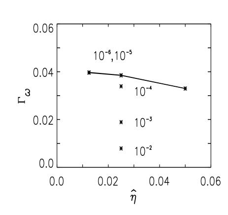
Figure 3: The parameter $\Gamma_{\omega}$ in Eq. (22) in its dependence on the inner radius $\hat{\eta}$ and the magnetic Prandtl number $\rm Pm$ (marking numbers). The $\rm Pm$-dependence disappears for small $\rm Pm$. The values hold for all containers with small inner radius. For $\rm Pm=1$ it is $\Gamma_{\omega}=0.0009$.

For $\rm Pm=10^{-6}$ we take from Fig. 3 the value $\Gamma_{\omega}=0.041$. Hence,

$$\omega_{\rm gr}=2.0\times\!10^{-3}B^{2}_{100}\,,$$ (24)

which yields

$$\tau_{\rm gr}=\frac{500}{B_{100}^{2}}$$ (25)

(with $B_{100}=B_{\rm out}/100\,{\rm G}$) as the growth time in seconds for the TI in gallium experiments. The size of the container does no longer influence the growth rate. The growth time for $B_{\rm out}=1$ kG now results to 5 s – and to ${\sim\!2}$ min for, say, 200 G.

5 Rotating container

Figure 4 gives for the wide-gap container the rotational quenching of the TI for various values of the magnetic Prandtl number. The lines for marginal instability in the $\rm Rm^{*}$-$\rm Ha_{\rm crit}$ plane are rather straight lines. The line for $\rm Pm=1$ gives the maximum stabilization by rigid rotation. In this representation a stronger stabilization does not exist. If ${\rm Rm^{*}}\lower 1.72218pt\hbox{$\;\buildrel<\over{\scriptstyle\sim}\;$}4\cdot{\rm Ha}$ then all fluids are unstable even under the influence of rotation. Note that the rotational stabilization is much weaker for $\rm Pm\neq 1$. It is particularly weak for very small $\rm Pm$.

Figure 4: The suppression of TI by uniform rotation for $\hat{\eta}=0.05$. The curves are marked with their magnetic Prandtl numbers. In this representation fluids with $\rm Pm=1$ undergo the strongest stabilization by rotation. The critical Hartmann number for resting container is 0.31 for all Pm.

We find from Fig. 4 that for fast rotation the magnetic Mach number (Eq. 11) is almost constant for given $\rm Pm$ (with minimum for $\rm Pm=1$) but still depends on the value of $\hat{\eta}$. We then also find that the quantity

$$\rm M=\sqrt{\hat{\eta}}\ Mm$$ (26)

does no longer depend on $\hat{\eta}$ but that it still slightly depends on $\rm Pm$ (Fig. 5). From Eq. (26) it results that

$${\it\Omega}={\rm M}\ {\it\Omega}_{\rm A}$$ (27)

is the critical rotation rate which stabilizes the TI. Here, the Alfvén frequency (Eq. 20) of the outer magnetic field amplitude has been used.

Figure 5: The same as in Fig. 4 but valid for $\hat{\eta}\to 0$. Note that fluids with $\rm Pm=1$ can be stabilized with the smallest rotation rates.

The question is whether the rotational stabilization of the TI can be probed in the laboratory. The rigidly rotating wide-gap container with ${\hat{\eta}=0.05}$ is thus considered also for the very small magnetic Prandtl numbers of fluid metals and for Reynolds numbers of order 10³ where after Fig. 4 the bifurcation lines are no longer straight lines. The magnetic Prandtl number of sodium is about ${\rm Pm=10^{-5}}$, and for gallium it is about ${\rm Pm=10^{-6}}$. Without rotation the critical Hartmann number is 0.31 for this container (independent of Pm). With rotation the numerical results are given in Fig. 6. We find the rotational stabilization also existing for conducting fluids with their very small Pm. For not too fast rotation the differences of the resulting critical Ha are very small for both the fluid conductors so that experiments with gallium or sodium are possible. For the small Reynolds number of order 1000 the marginal-stable magnetic field is about two times higher than for $\rm Re=0$. With the density (${\rho=6.4}$ g/cm³), viscosity ($\nu=3.4\!\times\!10^{-3}$  cm²/s) and magnetic diffusivity ($\eta=2428$ cm²/s) for Gallistan the corresponding magnetic field amplitudes (at the outer cylinder) in Gauss and the rotation frequencies (in Hz) are also given in Fig. 6. The resulting values are moderate. It should thus not be too complicated to find the basic effect of the rotational suppression of TI also in the MHD laboratory.

Figure 6: The suppression of the TI in a wide-gap container by rigid rotation for $\rm Pm=10^{-5}$ and $\rm Pm=10^{-6}$. The standard Reynolds number (8) is given for experimental applications. The numerical values of the outer field strength and the critical rotation rates are given for experiments with Gallistan. $\hat{\eta}=0.05$, $\mu_{B}=20$.

Our linear code is also able to work with ${\rm Pm}=0$. The curves in Fig. 6 do not become more steep for $\rm Pm\to 0$. There is no visible difference between the curves for ${\rm Pm}=10^{-6}$ and ${\rm Pm}=0$.

Figure 6 does not concern to a gallium column without inner cylinder. However, as demonstrated above the transition from $\hat{\eta}=0.05$ to $\hat{\eta}=0$ is easy. We take from Fig. 6 that close to the critical Hartmann number for resting container

$$\rm Re=\gamma_{\Omega}(Ha-Ha_{\rm crit})^{2.5}.$$ (28)

After the usual transformation to $B_{\rm out}$ one finds

$${\it\Omega}\simeq\Gamma_{\Omega}\ (\frac{B_{\rm out}}{\sqrt{\mu_{0}\rho}})^{5/2}\frac{R_{\rm out}^{1/2}}{{\rm Pm}^{1/4}\eta^{3/2}}$$ (29)

with $\Gamma_{\Omega}={\hat{\eta}}^{11/4}\ \gamma_{\omega}$. The result (29) also holds for $\hat{\eta}\to 0$. Figure 7 shows the numerical values of $\Gamma_{\Omega}$ for the fluids with small magnetic Prandtl numbers.

Figure 7: The parameter $\Gamma_{\Omega}$ for $\rm Pm=10^{-5}$ (long line) and $\rm Pm=10^{-6}$ (short line).

Using the numerical result $\Gamma_{\Omega}\simeq 4$ from Fig. 7 Eq. (29) yields

$${\it\Omega}\simeq 1.36\,B_{100}^{2.5}\quad[{\rm s}^{-1}]$$ (30)

for a container filled with Gallistan and with ${R_{\rm out}=5}$ cm or, what is the same, ${f=0.22\,B_{100}^{2.5}}$ as the critical rotation frequency which marginally stabilizes the TI. Hence, for (say) 200 Gauss the limit frequency is 1.2 Hz. which is much faster in comparison to the container with $\hat{\eta}=0.05$.

The influence of the rotation on the growth rates of the instability is only small. Figure 8 displays for $\rm Pm=10^{-6}$ the normalized growth rates for ${\rm Re=0}$ (solid line) and $\rm Re=1000$ (dashed line). The stabilizing action of the basic rotation is obvious.

Figure 8: The normalized growth rates for ${\rm Pm=10^{-6}}$ under the influence of rigid rotation with ${\rm Re=1000}$ (dashed). The solid line gives the growth rates for the resting container (see Fig. 2). Note the stabilizing action of global rotation. $\hat{\eta}=0.05$, $\mu_{B}=20$.

6 The magnetic field pattern

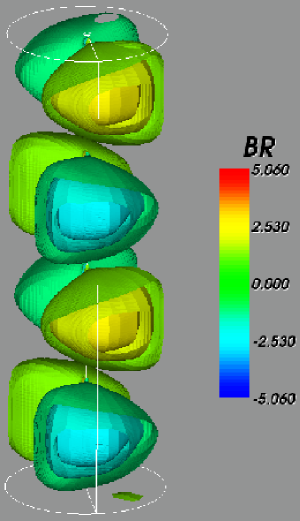
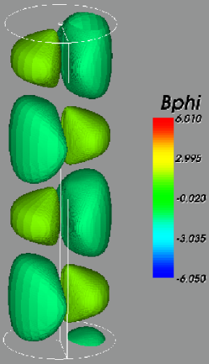
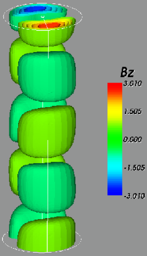
Figure 9: (online colour at: www.an-journal.org) Isosurface plots of all field components. The outermost visible surface represents 25 % of the maximum value. $\rm Re=0$, $\rm Ha=2$, $\hat{\eta}=0.05$, $\mu_{B}=20$, $\rm Pm=0.02$.

Without rotation the primary current-driven instability leads to a nondrifting steady-state solution. Isosurfaces of the pattern resulting from a 3D nonlinear simulation are shown in Fig. 9 for all the three field components. More details of the code which solves the incompressible MHD equations are given by Gellert et al. (2008). The boundary conditions at the walls are those for pseudovacuum. The container with $\hat{\eta}=0.05$ is periodic in $z$-direction with a domain height of $2\pi(R_{\rm out}-R_{\rm in})$. The Prandtl number $\rm Pm=0.02$ is the minimum value with which the code can operate. The Hartmann number ($\rm Ha=2$) is supercritical with almost two times the critical value. The dominating modes with $m=\pm 1$ lead to a kidney-shaped pattern. Note the different azimuthal angles of the pattern of the azimuthal component compared to the others.

From linear calculations we know that for smaller $\rm Pm$ the axial wave numbers decrease and the pattern extensions in axial direction become larger.

The secondary bifurcation leads to axial oscillations around half the wavelength. To what extent this picture holds for ${\mathrm{Pm}=10^{-6}}$ is open. Because of the $\mathrm{Pm}$-independent critical $\mathrm{Ha}$ and the only slightly larger Hartmann number used in the simulations shown here, it is possible that liquid metal experiments behave nearly the same.

7 A short review

The interplay of toroidal magnetic fields and solid-body rotation for incompressible fluids of uniform density filling the gap between the cylinders of a Taylor-Couette container is considered. The toroidal field is the result of an electric axial current of homogeneous density. It is shown that for zero rotation the critical magnetic field amplitudes for marginal Tayler instability do not depend on the magnetic Prandtl number. The critical magnetic field at the inner cylinder strongly depends on the gap width. It is very high for small gaps and it this rather low for wide gaps. For small enough inner radius $R_{\rm in}$ the critical Hartmann number (of the inner field strength) runs as $R_{\rm in}^{1.5}$. Note, however, that the critical magnetic field at the outer cylinder does hardly vary with the gap width (see Eq. 17). The resulting electric currents necessary for TI with $|m|=1$ slightly exceeds 3.2 kA if the material is the same gallium-tin alloy (GaInSn) as used in the experiment PROMISE. Such currents can easily be produced in the laboratory. The main difficulty for experiments is given by the long growth times of the instability for magnetic fields weaker than 1 kG.

Also the rotational quenching of the TI is studied. Figure 4 shows the rotational stabilization for various magnetic Prandtl numbers. To normalize the basic rotation a ‘mixed’ Reynolds number (Eq. 10) is used in which – as in the Hartmann number – the viscosities $\nu$ and $\eta$ are symmetric. The ratio of this Reynolds number and the Hartmann number (i.e. the magnetic Mach number) is free of any diffusivity. This ratio describes the rotational quenching of TI for various Pm. It is shown that the most effective stabilization of TI happens for ${\rm Pm=1}$. It is weaker for both smaller Pm and higher Pm. Many numerical simulations with $\rm Pm\simeq 1$, therefore, could overlook the nonaxisymmetric instability of strong toroidal fields.

Our calculations demonstrate that rigid rotation always stabilizes the magnetic field against the nonaxisymmetric TI. We have also shown that this rotational stabilization should be observable in the laboratory. Figure 6 provides the result that the critical Hartmann number in a wide-gap container of $\hat{\eta}=0.05$ can be increased by a factor of two by a rigid rotation of only a few Hz.

- [1] Acheson, D.J.: 1978, Phil. Trans. R. Soc. London A 289, 459
- [2] Chandrasekhar, S.: 1961, Hydrodynamic and Hydromagnetic Stability, Clarendon Press, Oxford
- [3] Chanmugam, G.: 1979, MNRAS 187, 769
- [4] Dubrulle, B., Knobloch, E.: 1993, A&A 274, 667
- [5] Howard, L.N., Gupta, A.S.: 1962, JFM 14, 463
- [6] Knobloch, E.: 1992, MNRAS 255, 25
- [7] Kumar, S., Coleman, C.S., Kley, W.: 1994, MNRAS 266, 379
- [8] Maeder, A., Meynet, G.: 2005, A&A 440, 1041
- [9] Michael, D.H.: 1954, Mathematika 1, 45
- [10] Pessah, M.E., Psaltis, D.: 2005, ApJ 628, 879
- [11] Pitts, E., Tayler, R.J.: 1985, MNRAS 216, 139
- [12] Roberts, P.H.: 1956, ApJ 124, 430
- [13] Rüdiger, G., Schultz, M.: 2010, AN 331, 121
- [14] Rüdiger, G., Hollerbach, R., Schultz, M., Elstner, D.: 2007a, MNRAS 377, 1481
- [15] Rüdiger, G., Schultz, M., Shalybkov, D., Hollerbach, R.: 2007b, Phys. Rev. E 76, 056309
- [16] Shalybkov, D.: 2006, Phys. Rev. E 73, 016302
- [17] Shalybkov, D., Rüdiger, G., Schultz, M.: 2002, A&A 395, 339
- [18] Tayler, R.J.: 1957, Proc. Phys. Soc. B 70, 31
- [19] Tayler, R.J.: 1973, MNRAS 161, 365
- [20] Vandakurov, Yu.V.: 1972, SvA 16, 265
- [21]