$T_{13}$ Flavor Symmetry and Decaying Dark Matter

Yuji Kajiyama^a,b and Hiroshi Okada^c,

^aNational Institute of Chemical Physics and Biophysics,
Ravala 10, Tallinn 10143, Estonia
^bDepartment of Physics, Niigata University, Niigata 950-2128, Japan
^cCentre for Theoretical Physics, The British University in Egypt,
El Sherouk City, Postal No, 11837, P.O. Box 43, Egypt

1 Introduction

Despite the great success of the Standard Model (SM) of the elementary particle physics, the origin of flavor structure, masses and mixings between generations, of matter particles are unknown yet. In order to overcome these problems, plenty of models based on the principle of symmetry, flavor symmetry, have been discussed. In particular, the fact that the lepton mixing matrix (Maki-Nakagawa-Sakata matrix) $U_{MNS}$ shows very good agreement with the tri-bi maximal form [1] implies that flavor structure is originated from a symmetry. Among them, non-Abelian discrete symmetries are well discussed as plausible possibilities [2].

On the other hand, it has been established that about 23 $\%$ of energy density of the universe consists of Dark Matter (DM) [3]. Indirect detection experiments of DM, PAMELA [4] and Fermi-LAT [5, 6], reported excess of positron and the total flux $(e^{+}+e^{-})$ in the cosmic ray. These observations can be explained by scattering and/or decay of TeV-scale DM particles. Since PAMELA measured negative results for anti-proton excess [7], leptophilic DM is preferable.

Even so, if the main final state of scattering or decay of DM is $\tau^{+}\tau^{-}$, this annihilation/decay mode is disfavored because it will overproduce gamma-rays as final state radiation [8]. This may indicate that if the cosmic-ray anomalies are induced by DM scattering or decay, these processes also reflect flavor structure of the theory. There are several papers in which the DM nature is related to flavor symmetry [9, 10, 11, 12, 13, 14, 15, 16].

While there are many models for the DM, we consider decaying DM model in this paper [17, 18, 19]. In such scenarios, no excess of anti-proton in the cosmic ray [7] implies that lifetime of the DM particle should be of ${\cal O}(10^{26})$ sec. This long lifetime is achieved if the TeV-scale DM (gauge singlet fermion $X$) decays into leptons by dimension six operators $\bar{L}E\bar{L}X/\Lambda^{2}$ suppressed by GUT scale $\Lambda\sim 10^{16}~{}\mbox{GeV}$ [18]. In this case, the lifetime of the DM is estimated as $\Gamma^{-1}\sim((\mbox{TeV})^{5}/\Lambda^{4})^{-1}\sim 10^{26}$ sec. However, in general, there are gauge invariant dimension four decay operators which induce rapid DM decay, and several dimension six operators which induce DM decay into quarks, Higgs and gauge bosons. Therefore one has to solve at least two problems for decaying DM models: i) why the lifetime of the DM is so long? ii) why the DM decays mainly into leptons? In ref. [9], we and our collaborators have shown that $A_{4}$ flavor symmetry can allow only the $\bar{L}E\bar{L}X/\Lambda^{2}$ operator and forbid the other undesirable operators, and determine flavor structure of DM decay mode. In that model, the $A_{4}$ symmetry allows only flavor universal leptonic decay mode, and the cosmic-ray anomalies are explained by fermionic DM decay.

In this paper, we show that similar argument is possible in $T_{13}$ flavor symmetry model as an extension of the $A_{4}$ model. The $T_{13}$ group, isomorphic to $Z_{13}\rtimes Z_{3}$ group, is non-Abelian discrete subgroup of $SU(3)$. For the lepton sector, tri-bi maximal form can be derived by embedding three generations into triplet representations of flavor symetries. In this point of view, $A_{4}$ is the minimal group which has a triplet, and the $T_{13}$ group has two complex triplets in the irreducible representations. However, since multiplication rules of the $T_{13}$ group is very different from those of $A_{4}$, we have a new texture of mass matrices of the lepton sector. As a result, although the $A_{4}$ model requires $SU(2)_{L}$ triplet Higgs bosons $\Delta$ with heavy mass $m_{\Delta}$ and small vacuum expectation values (VEVs) $v_{\Delta}$ to make the leptonic mixings and to suppress additional dimension five DM decay operator $H\Delta^{{\dagger}}\bar{L}X$, our $T_{13}$ model does not require $\Delta$. The DM decay operators are also constrained by the $T_{13}$ symmetry so that only $\bar{L}E\bar{L}X/\Lambda^{2}$ operators are allowed like $A_{4}$ model of ref. [9]. However unlike the $A_{4}$ model, DM decay mode depends on mixing matrices in general. In this paper we choose a particular set of parameters of the lepton sector, and show that the cosmic-ray anomalies can be well-explained by fermionic DM decay controlled by $T_{13}$ symmetry.

This paper is organized as follows. We briefly discuss group theory of $T_{13}$ and lists the multiplication rules in the next section. In the section 3, we construct mass matrices of the lepton sector in definite choice of $T_{13}$ assignment of the fields, and show that there exists a consistent set of parameters. In the section 4, we show that only desirable dimension six DM decay operators are allowed by $T_{13}$ symmetry and that leptonic decay of the DM by those operators shows good agreement with the cosmic-ray anomaly experiments. The section 5 is devoted to the conclusions.

2 $T_{13}$ group theory

First of all, we briefly review the non-Abelian discrete group $T_{13}$, which is isomorphic to $Z_{13}\rtimes Z_{3}$ [20, 21]. The $T_{13}$ group is a subgroup of $SU(3)$, and known as the minimal non-Abelian discrete group having two complex triplets as the irreducible representations. We denote the generators of $Z_{13}$ and $Z_{3}$ by $a$ and $b$, respectively. They satisfy

$$a^{13}=1,\quad ab=ba^{9}.$$ (2.1)

Using them, all of $T_{13}$ elements are written as

$$g=b^{m}a^{n},$$ (2.2)

with $m=0,1,2$ and $n=0,\cdots,12$.

The generators, $a$ and $b$, are represented e.g. as

$$b=\left(\begin{array}[]{ccc}0&1&0\\ 0&0&1\\ 1&0&0\\ \end{array}\right),\quad a=\left(\begin{array}[]{ccc}\rho&0&0\\ 0&\rho^{3}&0\\ 0&0&\rho^{9}\\ \end{array}\right),$$ (2.3)

where $\rho=e^{2i\pi/13}$. These elements are classified into seven conjugacy classes,

$$\begin{array}[]{ccc}C_{1}:&\{e\},&h=1,\\ C_{13}^{(1)}:&\{b~{},~{}ba~{},~{}ba^{2}~{},\quad...\quad,~{}ba^{10}~{},~{}ba^{11}~{},~{}ba^{12}\},&h=3,\\ C_{13}^{(2)}:&\{b^{2}~{},~{}b^{2}a~{},~{}b^{2}a^{2}~{},\quad...\quad,~{}b^{2}a^{10}~{},~{}b^{2}a^{11}~{},~{}b^{2}a^{12}\},&h=3,\\ C_{3_{1}}:&\{a~{},~{}a^{3}~{},~{}a^{9}\},&h=13,\\ C_{\bar{3}_{1}}:&\{a^{4}~{},~{}a^{10}~{},~{}a^{12}\},&h=13,\\ C_{3_{2}}:&\{a^{2}~{},~{}a^{5}~{},~{}a^{6}\},&h=13,\\ C_{\bar{3}_{2}}:&\{a^{7}~{},~{}a^{8}~{},~{}a^{11}\},&h=13.\\ \end{array}$$ (2.11)

The $T_{13}$ group has three singlets ${\bf 1}_{k}$ with $k=0,~{}1,~{}2$ and two complex triplets ${\bf 3_{1}}$ and ${\bf 3_{2}}$ as irreducible representations. The characters are shown in Table 1, where $\xi_{1}\equiv\rho+\rho^{3}+\rho^{9}$, $\xi_{2}\equiv\rho^{2}+\rho^{5}+\rho^{6}$, and $\omega\equiv e^{2i\pi/3}$.

	$n$	$h$	$\chi_{\bf 1_{0}}$	$\chi_{\bf 1_{1}}$	$\chi_{\bf 1_{2}}$	$\chi_{\bf 3_{1}}$	$\chi_{\bf\bar{3}_{1}}$	$\chi_{\bf 3_{2}}$	$\chi_{\bf\bar{3}_{2}}$
$C^{(0)}_{1}$	$1$	$1$	$1$	$1$	$1$	$3$	$3$	$3$	$3$
$C^{(1)}_{13}$	$13$	$3$	$1$	$\omega$	$\omega^{2}$	$0$	$0$	$0$	$0$
$C^{(2)}_{13}$	$13$	$3$	$1$	$\omega^{2}$	$\omega$	$0$	$0$	$0$	$0$
$C_{3_{1}}$	$3$	$13$	$1$	$1$	$1$	$\xi_{1}$	$\bar{\xi}_{1}$	$\xi_{2}$	$\bar{\xi}_{2}$
$C_{\bar{3}_{1}}$	$3$	$13$	$1$	$1$	$1$	$\bar{\xi}_{1}$	$\xi_{1}$	$\bar{\xi}_{2}$	$\xi_{2}$
$C_{3_{2}}$	$3$	$13$	$1$	$1$	$1$	$\xi_{2}$	$\bar{\xi}_{2}$	$\xi_{1}$	$\bar{\xi}_{1}$
$C_{\bar{3}_{2}}$	$3$	$13$	$1$	$1$	$1$	$\bar{\xi}_{2}$	$\xi_{2}$	$\bar{\xi}_{1}$	$\xi_{1}$

Table 1: Characters of $T_{13}$. $\bar{\xi}_{i}$ is defined as the complex conjugate of $\xi_{i}$.

Next we show the multiplication rules of the $T_{13}$ group. We define the triplets as

$${\bf 3_{1}}\equiv\left(\begin{array}[]{c}x_{1}\\ x_{3}\\ x_{9}\\ \end{array}\right),\quad{\bf\bar{3}_{1}}\equiv\left(\begin{array}[]{c}\bar{x}_{12}\\ \bar{x}_{10}\\ \bar{x}_{4}\\ \end{array}\right),\quad{\bf 3_{2}}=\left(\begin{array}[]{c}y_{2}\\ y_{6}\\ y_{5}\\ \end{array}\right),\quad{\bf\bar{3}_{2}}\equiv\left(\begin{array}[]{c}\bar{y}_{11}\\ \bar{y}_{7}\\ \bar{y}_{8}\\ \end{array}\right),$$ (2.24)

where the subscripts denote $Z_{13}$ charge of each element.

The tensor products between triplets are obtained as

$$\left(\begin{array}[]{c}x_{1}\\ x_{3}\\ x_{9}\\ \end{array}\right)_{{\bf 3_{1}}}\otimes\left(\begin{array}[]{c}y_{1}\\ y_{3}\\ y_{9}\\ \end{array}\right)_{{\bf 3_{1}}} = \left(\begin{array}[]{c}x_{3}y_{9}\\ x_{9}y_{1}\\ x_{1}y_{3}\\ \end{array}\right)_{{\bf\bar{3}_{1}}}\oplus\left(\begin{array}[]{c}x_{9}y_{3}\\ x_{1}y_{9}\\ x_{3}y_{1}\\ \end{array}\right)_{{\bf\bar{3}_{1}}}\oplus\left(\begin{array}[]{c}x_{1}y_{1}\\ x_{3}y_{3}\\ x_{9}y_{9}\\ \end{array}\right)_{{\bf 3_{2}}},$$ (2.40)

$$\left(\begin{array}[]{c}\bar{x}_{12}\\ \bar{x}_{10}\\ \bar{x}_{4}\\ \end{array}\right)_{{\bf\bar{3}_{1}}}\otimes\left(\begin{array}[]{c}\bar{y}_{12}\\ \bar{y}_{10}\\ \bar{y}_{4}\\ \end{array}\right)_{{\bf\bar{3}_{1}}} = \left(\begin{array}[]{c}\bar{x}_{10}\bar{y}_{4}\\ \bar{x}_{4}\bar{y}_{12}\\ \bar{x}_{12}\bar{y}_{10}\\ \end{array}\right)_{{\bf 3_{1}}}\oplus\left(\begin{array}[]{c}\bar{x}_{4}\bar{y}_{10}\\ \bar{x}_{12}\bar{y}_{4}\\ \bar{x}_{10}\bar{y}_{12}\\ \end{array}\right)_{{\bf 3_{1}}}\oplus\left(\begin{array}[]{c}\bar{x}_{12}\bar{y}_{12}\\ \bar{x}_{10}\bar{y}_{10}\\ \bar{x}_{4}\bar{y}_{4}\\ \end{array}\right)_{{\bf\bar{3}_{2}}},$$ (2.56)

$$\left(\begin{array}[]{c}x_{1}\\ x_{3}\\ x_{9}\\ \end{array}\right)_{{\bf 3_{1}}}\otimes\left(\begin{array}[]{c}\bar{y}_{12}\\ \bar{y}_{10}\\ \bar{y}_{4}\\ \end{array}\right)_{{\bf\bar{3}_{1}}} = \sum_{k=0,1,2}(x_{1}\bar{y}_{12}+\omega^{k}x_{3}\bar{y}_{10}+\omega^{2k}x_{9}\bar{y}_{4})_{{\bf 1}_{k}}\oplus\left(\begin{array}[]{c}x_{3}\bar{y}_{12}\\ x_{9}\bar{y}_{10}\\ x_{1}\bar{y}_{4}\\ \end{array}\right)_{{\bf 3_{2}}}\oplus\left(\begin{array}[]{c}x_{1}\bar{y}_{10}\\ x_{3}\bar{y}_{4}\\ x_{9}\bar{y}_{12}\\ \end{array}\right)_{{\bf\bar{3}_{2}}},$$ (2.69)

$$\left(\begin{array}[]{c}x_{2}\\ x_{6}\\ x_{5}\\ \end{array}\right)_{{\bf 3_{2}}}\otimes\left(\begin{array}[]{c}y_{2}\\ y_{6}\\ y_{5}\\ \end{array}\right)_{{\bf 3_{2}}} = \left(\begin{array}[]{c}x_{5}y_{6}\\ x_{2}y_{5}\\ x_{6}y_{2}\\ \end{array}\right)_{{\bf\bar{3}_{2}}}\oplus\left(\begin{array}[]{c}x_{6}y_{5}\\ x_{5}y_{2}\\ x_{2}y_{6}\\ \end{array}\right)_{{\bf\bar{3}_{2}}}\oplus\left(\begin{array}[]{c}x_{6}y_{6}\\ x_{5}y_{5}\\ x_{2}y_{2}\\ \end{array}\right)_{{\bf\bar{3}_{1}}},$$ (2.86)

$$\left(\begin{array}[]{c}\bar{x}_{11}\\ \bar{x}_{7}\\ \bar{x}_{8}\\ \end{array}\right)_{{\bf\bar{3}_{2}}}\otimes\left(\begin{array}[]{c}\bar{y}_{11}\\ \bar{y}_{7}\\ \bar{y}_{8}\\ \end{array}\right)_{{\bf\bar{3}_{2}}} = \left(\begin{array}[]{c}\bar{x}_{8}\bar{y}_{7}\\ \bar{x}_{11}\bar{y}_{8}\\ \bar{x}_{7}\bar{y}_{11}\\ \end{array}\right)_{{\bf 3_{2}}}\oplus\left(\begin{array}[]{c}\bar{x}_{7}\bar{y}_{8}\\ \bar{x}_{8}\bar{y}_{11}\\ \bar{x}_{11}\bar{y}_{7}\\ \end{array}\right)_{{\bf 3_{2}}}\oplus\left(\begin{array}[]{c}\bar{x}_{7}\bar{y}_{7}\\ \bar{x}_{8}\bar{y}_{8}\\ \bar{x}_{11}\bar{y}_{11}\\ \end{array}\right)_{{\bf 3_{1}}},$$ (2.102)

$$\left(\begin{array}[]{c}x_{2}\\ x_{6}\\ x_{5}\\ \end{array}\right)_{{\bf 3_{2}}}\otimes\left(\begin{array}[]{c}\bar{y}_{11}\\ \bar{y}_{7}\\ \bar{y}_{8}\\ \end{array}\right)_{{\bf\bar{3}_{2}}} = \sum_{k=0,1,2}(x_{2}\bar{y}_{11}+\omega^{k}x_{6}\bar{y}_{7}+\omega^{2k}x_{5}\bar{y}_{8})_{{\bf 1}_{k}}\oplus\left(\begin{array}[]{c}x_{6}\bar{y}_{8}\\ x_{5}\bar{y}_{11}\\ x_{2}\bar{y}_{7}\\ \end{array}\right)_{{\bf 3_{1}}}\oplus\left(\begin{array}[]{c}x_{5}\bar{y}_{7}\\ x_{2}\bar{y}_{8}\\ x_{6}\bar{y}_{11}\\ \end{array}\right)_{{\bf\bar{3}_{1}}},$$ (2.115)

$$\left(\begin{array}[]{c}x_{1}\\ x_{3}\\ x_{9}\\ \end{array}\right)_{{\bf 3_{1}}}\otimes\left(\begin{array}[]{c}y_{2}\\ y_{6}\\ y_{5}\\ \end{array}\right)_{{\bf 3_{2}}} = \left(\begin{array}[]{c}x_{9}y_{6}\\ x_{1}y_{5}\\ x_{3}y_{2}\\ \end{array}\right)_{{\bf 3_{2}}}\oplus\left(\begin{array}[]{c}x_{9}y_{2}\\ x_{1}y_{6}\\ x_{3}y_{5}\\ \end{array}\right)_{{\bf\bar{3}_{2}}}\oplus\left(\begin{array}[]{c}x_{9}y_{5}\\ x_{1}y_{2}\\ x_{3}y_{6}\\ \end{array}\right)_{{\bf 3_{1}}},$$ (2.132)

$$\left(\begin{array}[]{c}x_{1}\\ x_{3}\\ x_{9}\\ \end{array}\right)_{{\bf 3_{1}}}\otimes\left(\begin{array}[]{c}\bar{y}_{11}\\ \bar{y}_{7}\\ \bar{y}_{8}\\ \end{array}\right)_{{\bf\bar{3}_{2}}} = \left(\begin{array}[]{c}x_{1}\bar{y}_{11}\\ x_{3}\bar{y}_{7}\\ x_{9}\bar{y}_{8}\\ \end{array}\right)_{{\bf\bar{3}_{1}}}\oplus\left(\begin{array}[]{c}x_{3}\bar{y}_{8}\\ x_{9}\bar{y}_{11}\\ x_{1}\bar{y}_{7}\\ \end{array}\right)_{{\bf\bar{3}_{2}}}\oplus\left(\begin{array}[]{c}x_{3}\bar{y}_{11}\\ x_{9}\bar{y}_{7}\\ x_{1}\bar{y}_{8}\\ \end{array}\right)_{{\bf 3_{1}}},$$ (2.148)

$$\left(\begin{array}[]{c}x_{2}\\ x_{6}\\ x_{5}\\ \end{array}\right)_{{\bf 3_{2}}}\otimes\left(\begin{array}[]{c}\bar{y}_{12}\\ \bar{y}_{10}\\ \bar{y}_{4}\\ \end{array}\right)_{{\bf\bar{3}_{1}}} = \left(\begin{array}[]{c}x_{2}\bar{y}_{12}\\ x_{6}\bar{y}_{10}\\ x_{5}\bar{y}_{4}\\ \end{array}\right)_{{\bf 3_{1}}}\oplus\left(\begin{array}[]{c}x_{2}\bar{y}_{10}\\ x_{6}\bar{y}_{4}\\ x_{5}\bar{y}_{12}\\ \end{array}\right)_{{\bf\bar{3}_{1}}}\oplus\left(\begin{array}[]{c}x_{5}\bar{y}_{10}\\ x_{2}\bar{y}_{4}\\ x_{6}\bar{y}_{12}\\ \end{array}\right)_{{\bf 3_{2}}},$$ (2.164)

$$\left(\begin{array}[]{c}\bar{x}_{12}\\ \bar{x}_{10}\\ \bar{x}_{4}\\ \end{array}\right)_{{\bf\bar{3}_{1}}}\otimes\left(\begin{array}[]{c}\bar{y}_{11}\\ \bar{y}_{7}\\ \bar{y}_{8}\\ \end{array}\right)_{{\bf\bar{3}_{2}}} = \left(\begin{array}[]{c}\bar{x}_{4}\bar{y}_{8}\\ \bar{x}_{12}\bar{y}_{11}\\ \bar{x}_{10}\bar{y}_{7}\\ \end{array}\right)_{{\bf\bar{3}_{1}}}\oplus\left(\begin{array}[]{c}\bar{x}_{4}\bar{y}_{7}\\ \bar{x}_{12}\bar{y}_{8}\\ \bar{x}_{10}\bar{y}_{11}\\ \end{array}\right)_{{\bf\bar{3}_{2}}}\oplus\left(\begin{array}[]{c}\bar{x}_{4}\bar{y}_{11}\\ \bar{x}_{12}\bar{y}_{7}\\ \bar{x}_{10}\bar{y}_{8}\\ \end{array}\right)_{{\bf 3_{2}}}.$$ (2.180)

The tensor products between singlets are obtained as

$$(x)_{{\bf 1}_{0}}(y)_{{\bf 1}_{0}}=(x)_{{\bf 1}_{1}}(y)_{{\bf 1}_{2}}=(x)_{{\bf 1}_{2}}(y)_{{\bf 1}_{1}}=(xy)_{{\bf 1}_{0}},~{}$$

$$(x)_{{\bf 1}_{1}}(y)_{{\bf 1}_{1}}=(xy)_{{\bf 1}_{2}},~{}(x)_{{\bf 1}_{2}}(y)_{{\bf 1}_{2}}=(xy)_{{\bf 1}_{1}}.$$ (2.181)

The tensor products between triplets and singlets are obtained as

$$(y)_{{\bf 1}_{k}}\otimes\left(\begin{array}[]{c}x(\bar{x})_{1}\\ x(\bar{x})_{2}\\ x(\bar{x})_{3}\\ \end{array}\right)_{{\bf 3(\bar{3})}}=\left(\begin{array}[]{c}yx(\bar{x})_{1}\\ yx(\bar{x})_{2}\\ yx(\bar{x})_{3}\\ \end{array}\right)_{{\bf 3(\bar{3})}}.$$ (2.188)

In the following section, we discuss mass matrices of the lepton sector determined by the $T_{13}$ flavor symmetry.

3 Lepton masses and mixings

In this section, we discuss the lepton masses and mixings in the setup shown in Table 2. Here, $Q$, $U$, $D$, $L$, $E$, $H(H^{\prime})$ and $X$ denote left-handed quarks, right-handed up-type quarks, right-handed down-type quarks, left-handed leptons, right-handed charged leptons, Higgs bosons, and gauge singlet fermion, respectively. We introduce two $T_{13}$ triplet Higgs bosons $H({\bf 3_{1}})$ and $H({\bf\bar{3}_{2}})$ which couple to leptons, and three $T_{13}$ singlet Higgs bosons $H^{\prime}({\bf 1_{0,1,2}})$ couple to quarks. This is realized by appropriate choice of an additional $Z_{3}$ symmetry. Since we concentrate on the lepton sector in this paper, $T_{13}$ charge of quarks and $H^{\prime}$ are assigned to the singlets. Therefore, mass matrices in the quark sector are not constrained, while those in the lepton sector are determined by the $T_{13}$ symmetry. A gauge and $T_{13}$ singlet fermion $X$ is also introduced in addition to the SM matter fermions. Since the Yukawa couplings $LXH$ are forbidden by the $T_{13}$ symmetry, this new fermion $X$ does not work as right-handed neutrino, and left-handed Majorana neutrino mass terms are generated by dimension five operators $LHLH$. The fermion $X$ is a DM candidate decaying into leptons by dimension six operators $\bar{L}E\bar{L}X$. However, we postpone the discussion on this point to the next section.

For the matter content and the $T_{13}$ assignment given in Table 2, the charged-lepton and neutrino masses are generated from the $T_{13}$ invariant operators

$${\cal L}_{Y} = \sqrt{2}a_{e}\bar{E}LH^{c}({\bf\bar{3}_{2}})+\sqrt{2}b_{e}\bar{E}LH^{c}({\bf 3_{1}})$$ (3.1)

$$+ \frac{a_{\nu}}{\Lambda}LH({\bf\bar{3}_{2}})LH({\bf\bar{3}_{2}})+\frac{b_{\nu}}{\Lambda}LH({\bf\bar{3}_{2}})LH({\bf 3_{1}})+\frac{c_{\nu}}{\Lambda}LH({\bf\bar{3}_{2}})LH({\bf 3_{1}})+h.c.,$$

where $H^{c}=\epsilon H^{*}$ and the fundamental scale $\Lambda=10^{11}~{}\mbox{GeV}$. After the electroweak symmetry breaking, the Lagrangian Eq.(3.1) gives rise to mass matrices of charged leptons $M_{e}$ and neutrinos $M_{\nu}$

$$M_{e} = \left(\begin{array}[]{ccc}0&b_{e}v_{1}&a_{e}\bar{v}_{2}\\ a_{e}\bar{v}_{3}&0&b_{e}v_{2}\\ b_{e}v_{3}&a_{e}\bar{v}_{1}&0\\ \end{array}\right),~{}$$ (3.5)

$$M_{\nu} = \frac{1}{\Lambda}\left(\begin{array}[]{ccc}c_{\nu}\bar{v}_{3}v_{2}&a_{\nu}\bar{v}_{1}^{2}+b_{\nu}\bar{v}_{3}v_{1}&a_{\nu}\bar{v}_{3}^{2}+b_{\nu}\bar{v}_{2}v_{3}\\ a_{\nu}\bar{v}_{1}^{2}+b_{\nu}\bar{v}_{3}v_{1}&c_{\nu}\bar{v}_{1}v_{3}&a_{\nu}\bar{v}_{2}^{2}+b_{\nu}\bar{v}_{1}v_{2}\\ a_{\nu}\bar{v}_{3}^{2}+b_{\nu}\bar{v}_{2}v_{3}&a_{\nu}\bar{v}_{2}^{2}+b_{\nu}\bar{v}_{1}v_{2}&c_{\nu}\bar{v}_{2}v_{1}\\ \end{array}\right),$$ (3.9)

where the VEVs are defined as

$$\langle H({\bf 3_{1}})^{i}\rangle=\frac{v_{i}}{\sqrt{2}},~{}\langle H({\bf\bar{3}_{2}})^{i}\rangle=\frac{\bar{v}_{i}}{\sqrt{2}},~{}\sum_{i=1}^{3}\left(v_{i}^{2}+\bar{v}_{i}^{2}\right)=(246~{}\mbox{GeV})^{2}.$$ (3.10)

	$Q$	$U$	$D$	$L$	$E$	$H$	$H^{\prime}$	$X$
$SU(2)_{L}\times U(1)_{Y}$	21/6	12/3	1-1/3	2-1/2	1-1	21/2	21/2	10
$T_{13}$	${\bf 1_{0,1,2}}$	${\bf 1_{0,1,2}}$	${\bf 1_{0,1,2}}$	${\bf 3_{1}}$	${\bf 3_{2}}$	${\bf 3_{1}},{\bf\bar{3}_{2}}$	${\bf 1_{0,1,2}}$	${\bf 1_{0}}$
$Z_{3}$	$1$	$\omega$	$\omega^{2}$	$1$	$1$	$1$	$\omega$	$1$

Table 2: The $T_{13}$ and $Z_{3}$ charge assignment of the SM fields and the dark matter $X$, where $\omega=e^{2i\pi/3}$.

Now we give a numerical example. By the following choice of parameters

$$v_{1} = 0.118297~{}\mbox{GeV},~{}v_{2}=179.257~{}\mbox{GeV},~{}v_{3}=1.99413~{}\mbox{GeV},$$ (3.11)

$$\bar{v}_{1} = 10~{}\mbox{GeV},~{}\bar{v}_{2}=168.164~{}\mbox{GeV},~{}\bar{v}_{3}=0.0483626~{}\mbox{GeV},$$

$$a_{e} = 0.010566,~{}b_{e}=0,~{}a_{\nu}=-9.71512\times 10^{-5},~{}b_{\nu}=5.19702\times 10^{-4},~{}c_{\nu}=0.169389,$$

the mass matrices Eqs. (3.5) and (3.9) give rise to mass eigenvalues and related observatives as

$$m_{e} = 0.511~{}\mbox{MeV},~{}m_{\mu}=105.66~{}\mbox{MeV},~{}m_{\tau}=1776.82~{}\mbox{MeV},$$

$$m_{\nu 1} = 1.385\times 10^{-2}~{}\mbox{eV},~{}m_{\nu 2}=1.637\times 10^{-2}~{}\mbox{eV},~{}m_{\nu 3}=5.194\times 10^{-2}~{}\mbox{eV},$$ (3.12)

$$\Delta m_{21}^{2} = m_{\nu 2}^{2}-m_{\nu 1}^{2}=7.59\times 10^{-5}~{}\mbox{eV}^{2},~{}\Delta m_{32}^{2}=m_{\nu 3}^{2}-m_{\nu 2}^{2}=2.43\times 10^{-3}~{}\mbox{eV}^{2},~{}$$

$$\langle m\rangle_{ee} = 1.47\times 10^{-2}~{}\mbox{eV},~{}\sum_{i}m_{\nu i}=8.2\times 10^{-2}~{}\mbox{eV},$$

and the mixing matrices

$$U_{eL} = \left(\begin{array}[]{ccc}1&0&0\\ 0&1&0\\ 0&0&1\\ \end{array}\right),~{}U_{eR}=\left(\begin{array}[]{ccc}0&0&1\\ 1&0&0\\ 0&1&0\\ \end{array}\right),~{}$$ (3.19)

$$U_{MNS} = U_{eL}^{{\dagger}}U_{\nu}=\left(\begin{array}[]{ccc}0.828521&0.558869&0.0348995\\ -0.374962&0.60001&-0.706676\\ -0.41588&0.57241&0.706676\\ \end{array}\right),$$ (3.23)

which are all consistent with the present experimental data [22]. In particular in the case of $U_{eL}=1$, the mass matrices Eqs. (3.5) and (3.9) require normal hierarchy $m_{\nu 1}<m_{\nu 2}<m_{\nu 3}$ of the neutrino masses and $U_{e3}^{MNS}\neq 0$. A comprehensive analysis of the $T_{13}$ symmetry models will be published elsewhere [23]. In the following analysis, we assume these parameters to discuss decaying dark matter.

4 Decaying dark matter in the $T_{13}$ model

The cosmic-ray anomalies measured by PAMELA [4] and Fermi-LAT [5, 6] can be explained by DM decay with lifetime of order $\Gamma^{-1}\sim 10^{26}$ sec. If the DM decays into leptons by dimension six operators $\bar{L}E\bar{L}X/\Lambda^{2}$, where $X$ is the gauge singlet fermionic DM, such long lifetime can be achieved. In general, however, there exist several gauge invariant decay operators of dimension four which induce rapid DM decay, and of dimension six which include quarks, Higgs and gauge bosons in the final states. In this section, we first show that the $T_{13}$ flavor symmetry forbids those undesired operators. Next we show by calculating the positron (electron) flux that the scenario, which has a particular generation structure of DM decay vertices, is possible to excellently describe the cosmic-ray anomalies.

4.1 Dark matter decay operators

Dimensions		DM decay operators
4		$\bar{L}H^{c}X$
5		$-$
6		$\bar{L}E\bar{L}X$,   $H^{\dagger}\!H\bar{L}H^{c}X$,   $(H^{c})^{t}D_{\mu}H^{c}\bar{E}\gamma^{\mu}X$,
		$\bar{Q}D\bar{L}X$,   $\bar{U}Q\bar{L}X$,   $\bar{L}D\bar{Q}X$,   $\bar{U}\gamma_{\mu}D\bar{E}\gamma^{\mu}X$,
		$D^{\mu}H^{c}D_{\mu}\bar{L}X$,   $D^{\mu}D_{\mu}H^{c}\bar{L}X$,
		$B_{\mu\nu}\bar{L}\sigma^{\mu\nu}H^{c}X$,   $W_{\mu\nu}^{a}\bar{L}\sigma^{\mu\nu}\tau^{a}H^{c}X$

Table 3: The decay operators of the gauge-singlet fermionic dark matter $X$ up to dimension six. $B_{\mu\nu}$, $W_{\mu\nu}^{a}$, and $D_{\mu}$ are the field strength tensor of hypercharge gauge boson, weak gauge boson, and the electroweak covariant derivative.

In our model, as mentioned before, a gauge-singlet fermion $X$ is introduced as the dark matter particle in addition to the SM fermions. By assuming that the baryon number is preserved at least at perturbative level, it turns out that there exist various gauge invariant operators up to dimension six shown in Table 3  [24] . From the table, one finds that the dark matter $X$ can in general decay into not only leptons but also quarks, Higgs, and gauge bosons at similar rates by dimension six operators. Furthermore, a rapid decay of DM is induced if the dimension four Yukawa operator $\bar{L}H^{c}X$ is allowed. One may try to impose an Abelian (continuous or discrete) symmetry to prohibit unwanted decay operators, but it is shown in ref. [9] that it does not work but $A_{4}$ flavor symmetry does. However in the $A_{4}$ model discussed in ref. [9], $SU(2)_{L}$ triplet Higgs bosons $\Delta$ are introduced in order to give the mixings of the lepton sector, and these give rise to dimension five DM decay operators. In order to avoid rapid DM decay by the dimension five operators, small VEVs $\langle\Delta\rangle$ and large mass $m_{\Delta}$ are required. On the other hand, lepton masses and mixings are generated only by $SU(2)_{L}$ doublet Higgs bosons in the $T_{13}$ model as shown in the section 3.

Remarkably, by the field assignment of Table 2, all the decay operators listed in Table 3 except for $\bar{L}E\bar{L}X$ are forbidden due to this single symmetry. Consequently the DM mainly decays into three leptons. With the notation $L_{i}=(\nu_{i},\ell_{i})=(U_{eL})_{i\alpha}(\nu_{\alpha},\ell_{\alpha})$ and $E_{i}=(U_{eR})_{i\beta}E_{\beta}$ $(i=1,2,3,~{}\alpha,\beta=e,\mu,\tau)$, the four-Fermi decay interaction is explicitly written as

$${\cal L}_{\rm decay} = \frac{\lambda}{\Lambda^{2}}\,\sum_{i=1}^{3}(\bar{L}_{i}E_{i})\bar{L}_{i}X\,+\text{h.c.}$$

$$= \frac{\lambda}{\Lambda^{2}}\sum_{i=1}^{3}\sum_{\alpha,\beta,\gamma=e,\mu,\tau}\left(U_{eL}\right)_{i\alpha}^{*}\left(U_{eR}\right)_{i\beta}\left(U_{eL}\right)_{i\gamma}^{*}$$

$$\left[\left(\bar{\nu}_{\alpha}P_{R}E_{\beta}\right)\left(\bar{\ell}_{\gamma}P_{R}X\right)-\left(\bar{\ell}_{\gamma}P_{R}E_{\beta}\right)\left(\bar{\nu}_{\alpha}P_{R}X\right)\right]+\text{h.c.}.$$

As seen from Eq. (4.1), decay mode of the DM particle $X$ depends on the mixing matrices $U_{e(L,R)}$, which are given in Eq. (3.19).

4.2 Positron production from dark matter decay

Next, we consider the branching fraction of the DM decay through the $T_{13}$ invariant Lagrangian Eq.(4.1). Due to the particular generation structure, the dark matter $X$ decays into several tri-leptons final state with the mixing-dependent rate. The decay width of DM per each flavor ($\Gamma_{\alpha\beta\gamma}\equiv\Gamma(X\to\nu_{\alpha}\ell^{+}_{\beta}\ell^{-}_{\gamma})$) turns out to be

$$\Gamma_{\alpha\beta\gamma} = \frac{|\lambda|^{2}m_{X}^{5}}{3072\pi^{3}\Lambda^{4}}\left(U_{\alpha\beta\gamma}+U_{\alpha\gamma\beta}\right),$$ (4.2)

where $m_{X}$ is the DM mass, and

$$U_{\alpha\beta\gamma}=\left|\sum_{i=1}^{3}\left(U_{eL}\right)_{i\alpha}^{*}\left(U_{eR}\right)_{i\beta}\left(U_{eL}\right)_{i\gamma}^{*}\right|^{2}.$$ (4.3)

Here we have omitted the masses of charged leptons in the final states. The flavor dependent factor $U_{\alpha\beta\gamma}$ gives a factor three if one takes the sum of flavor indices $\alpha,\beta$ and $\gamma$. Therefore, the branching fraction of each decay mode is given by

$$BR(X\to\nu_{\alpha}\ell^{+}_{\beta}\ell^{-}_{\gamma})=\frac{1}{6}\left(U_{\alpha\beta\gamma}+U_{\alpha\gamma\beta}\right).$$ (4.4)

The DM mass $m_{X}$ and the total decay width $\Gamma=\sum_{\alpha,\beta,\gamma}\Gamma_{\alpha\beta\gamma}$ are chosen to be free parameters in the following analysis.

Given the decay width and the branching fractions, the positron (electron) production rate (per unit volume and unit time) at the position $\vec{x}$ of the halo associated with our galaxy is evaluated as

$$Q(E,\vec{x})\,=\,n_{X}(\vec{x})\,\Gamma\sum_{f}{\rm Br}(X\to f)\bigg{[}\frac{dN_{e^{\pm}}}{dE}\bigg{]}_{f},$$ (4.5)

where $[dN_{e^{\pm}}/dE]_{f}$ is the energetic distribution of positrons (electrons) from the decay of single DM with the final state ‘$f$’. We use the PYTHIA code [25] to evaluate the distribution $[dN_{e^{\pm}}/dE]_{f}$. The DM number density $n_{X}(\vec{x})$ is obtained by the profile $\rho(\vec{x})$, the DM mass distribution in our galaxy, through the relation $\rho(\vec{x})=m_{X}n_{X}(\vec{x})$. In this work we adopt the Navarro-Frank-White profile [26],

$$\rho_{\rm NFW}(\vec{x})\,=\,\rho_{\odot}\frac{r_{\odot}(r_{\odot}+r_{c})^{2}}{r(r+r_{c})^{2}},$$ (4.6)

where $\rho_{\odot}\simeq 0.30$ GeV/cm³ is the local halo density around the solar system, $r$ is the distance from the galactic center whose special values $r_{\odot}\simeq 8.5$ kpc and $r_{c}\simeq 20$ kpc are the distance to the solar system and the core radius of the profile, respectively.

As seen from Eqs. (3.19) and (4.2), the DM decays into $\tau^{\pm}$ as well as $e^{\pm}$ and $\mu^{\pm}$ in the equal rate. However, $\tau^{\pm}$ in the final states decay into hadrons, and such hadronic decays are suppressed by the electroweak coupling and the phase space factor. As a result, pure leptonic decays give dominant contributions, and it is consistent with no anti-proton excess of the PAMELA results [7]. On the other hand, the injections of high-energy positrons (electrons) in the halo give rise to gamma rays through the bremsstrahlung and inverse Compton scattering processes. These gamma-ray flux [27] from leptonically decaying DM may constrain mass and lifetime of the DM [28, 29]. We will discuss this point later. Therefore, we concentrate on calculating the $e^{\pm}$ fluxes in what follows. We follow ref. [9] for diffusion model describing the propagation of positrons and electrons [30, 31, 32], and backgrounds [30, 33].

4.3 Results for PAMELA and Fermi-LAT

The positron fraction and the total flux $[\Phi_{e^{-}}]_{\text{total}}+[\Phi_{e^{+}}]_{\text{total}}$ are depicted in Figure 1 for the scenario of the leptonically decaying DM with $T_{13}$ symmetry. For the DM mass $m_{X}=2$, $2.5$, and $3$ TeV, the results are shown with the experimental data of PAMELA and Fermi-LAT. The total decay width $\Gamma$ is fixed for each value of DM mass so that the best fit value explains the experimental data. With a simple $\chi^{2}$ analysis, we obtain $\Gamma^{-1}=8.4\times 10^{25}$, $6.95\times 10^{25}$, and $5.9\times 10^{25}$ sec for $m_{X}=2.0$, $2.5$, and $3.0$ TeV, respectively. One can see that in the $m_{X}=2.5$ TeV case, both experiments are well explained in the $T_{13}$ model. Recent studies [28, 29] suggest that mass and lifetime of the decaying DM are strongly constrained by gamma-ray measurement from cluster of galaxies, and that allowed region which can simultaneously explain the PAMELA and Fermi-LAT results does not exist. To avoid these constraints, mass and lifetime of the DM should be lighter than $\sim{\cal O}(\mbox{TeV})$ and longer than $\sim{\cal O}(10^{27})$ sec, respectively. In that case, only the PAMELA results can be explained by the decaying DM.

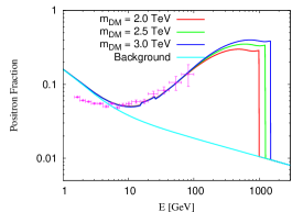
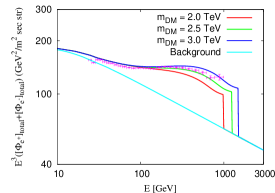
Figure 1: The positron fraction [4] and the total $e^{+}+e^{-}$ flux [5, 6] predicted in the leptonically-decaying DM scenario with $T_{13}$ symmetry. The DM mass is fixed to 2.0, 2.5, and 3.0 TeV. As for the DM decay width used in the fit, see the text.

5 Conclusions

We have considered a new flavor symmetric model based on a non-Abelian discrete symmetry $T_{13}$. The $T_{13}$ group, isomorphic to $Z_{13}\rtimes Z_{3}$, is the minimal group which contains two complex triplets in the irreducible representations. The form of mass matrices are determined by the assignment of $T_{13}$ charges and the multiplication rules. We have shown that masses and mixings in the lepton sector are derived in the $T_{13}$ model consistently. Thanks to the complexities of the $T_{13}$ group compared to $A_{4}$, both the leptonic masses and mixings are made only by $SU(2)_{L}$ doublet Higgs bosons.

We have also shown that the decay of gauge-singlet fermionic dark matter can explain the cosmic-ray anomalies reported by the PAMELA and Fermi-LAT experiments. It is known that if the dark matter is TeV-scale fermionic particle, its longevity of order $10^{26}$ sec can be derived from dimension six four-fermi operators suppressed by a large scale of new physics. The $T_{13}$ symmetry forbids DM decay of final states with quarks, Higgs and gauge bosons, and allows only leptonic decay. Moreover, it determines the DM decay mode so that tauon final state does not give dominant contribution. We found that due to the fermionic DM decay controlled by the $T_{13}$ flavor symmetry, the cosmic-ray anomalies are well-explained.

In this paper, we have explicitly given a numerical example of one consistent set of parameters in the mass matrices of the lepton sector. For completeness, a comprehensive analysis of mass matrices and its phenomenology in $T_{13}$ symmetric models will be published elsewhere [23].

Acknowledgments

We would like to thank N. Haba, S. Matsumoto, M. Raidal and K. Yoshioka for useful discussions. The work of Y.K. was supported by the ESF grant No. 8090 and Young Researcher Overseas Visits Program for Vitalizing Brain Circulation Japanese in JSPS. H.O. acknowledges partial supports from the Science and Technology Development Fund (STDF) project ID 437 and the ICTP project ID 30.

References

• [1] P. F. Harrison, D. H. Perkins, and W. G. Scott,  Phys. Lett. B530(2002) 167; P. F. Harrison and W. G. Scott, Phys. Lett. B535 (2002) 163.
• [2] For a review of non-Abelian discrete symmetry, H. Ishimori, T. Kobayashi, H. Ohki, H. Okada, Y. Shimizu and M. Tanimoto, Prog. Theor. Phys. Suppl. 183 (2010) 1.
• [3] E. Komatsu et al., arXiv:1001.4538 [astro-ph.CO].
• [4] O. Adriani et al., Nature 458 (2009) 607.
• [5] A.A. Abdo et al., Phys. Rev. Lett. 102 (2009) 181101 .
• [6] M. Ackermann et al., arXiv:1008.3999 [astro-ph.HE].
• [7] O. Adriani et al., Phys. Rev. Lett. 102 (2009) 051101.
• [8] M. Papucci and A. Strumia, JCAP 1003, 014 (2010).
• [9] N. Haba, Y. Kajiyama, S. Matsumoto, H. Okada and K. Yoshioka, Phys. Lett.  B 695, 476 (2011).
• [10] Y. Daikoku, H. Okada and T. Toma, arXiv:1010.4963 [hep-ph]; M. K. Parida, P. K. Sahu and K. Bora, arXiv:1011.4577 [hep-ph].
• [11] M. Hirsch, S. Morisi, E. Peinado and J. W. F. Valle, arXiv:1007.0871 [hep-ph].
• [12] D. Meloni, S. Morisi and E. Peinado, arXiv:1011.1371 [hep-ph].
• [13] J. N. Esteves, F. R. Joaquim, A. S. Joshipura, J. C. Romao, M. A. Tortola and J. W. F. Valle, Phys. Rev.  D 82 (2010) 073008.
• [14] Y. Kajiyama, J. Kubo and H. Okada, Phys. Rev.  D 75 (2007) 033001.
• [15] M. Schmaltz, Phys. Rev.  D 52 (1995) 1643.
• [16] Z. G. Berezhiani and M. Y. Khlopov, Z. Phys.  C 49 (1991) 73; H. Zhang, C. S. Li, Q. H. Cao and Z. Li, Phys. Rev.  D 82 (2010) 075003; M. Holthausen and R. Takahashi, Phys. Lett. B 691 (2010) 56.
• [17] A. Ibarra and D. Tran, JCAP 0902 (2009) 021; E. Nardi, F. Sannino and A. Strumia, JCAP 0901 (2009) 043; H. S. Goh, L. J. Hall and P. Kumar, JHEP 0905 (2009) 097; R. Essig, N. Sehgal and L.E. Strigari, Phys. Rev. D 80 (2009) 023506; D. Malyshev, I. Cholis and J. Gelfand, Phys. Rev. D 80 (2009) 063005; V. Barger, Y. Gao, W.Y. Keung, D. Marfatia and G. Shaughnessy, Phys. Lett. B 678 (2009) 283; P. Meade, M. Papucci, A. Strumia and T. Volansky, Nucl. Phys. B 831 (2010) 178; L. Zhang, G. Sigl and J. Redondo, JCAP 0909 (2009) 012; A. Ibarra, D. Tran and C. Weniger, JCAP 1001 (2010) 009; M. Cirelli, P. Panci and P. D. Serpico, Nucl. Phys. B 840 (2010) 284; L. Covi, M. Grefe, A. Ibarra and D. Tran, JCAP 1004 (2010) 017; L. Zhang, C. Weniger, L. Maccione, J. Redondo and G. Sigl, JCAP 1006(2010) 027; G. Hutsi, A. Hektor and M. Raidal, JCAP 1007 (2010) 008.
• [18] C. R. Chen, F. Takahashi and T. T. Yanagida, Phys. Lett.  B 673(2009) 255; A. Arvanitaki, S. Dimopoulos, S. Dubovsky, P.W. Graham, R. Harnik and S. Rajendran, Phys. Rev. D 79 (2009) 105022; Phys. Rev. D 80 (2009) 055011; K. Hamaguchi, S. Shirai and T. T. Yanagida, Phys. Lett. B 673 (2009) 247; B. Kyae, JCAP 0907 (2009) 028; P.H. Frampton and P.Q. Hung, Phys. Lett. B 675 (2009) 411; M. Kadastik, K. Kannike and M. Raidal, Phys. Rev. D 81 (2010) 015002; Phys. Rev. D 80 (2009) 085020; J.T. Ruderman and T. Volansky, arXiv:0907.4373 [hep-ph]; J.H. Huh and J.E. Kim, Phys. Rev. D 80 (2009) 075012; M. Luo, L. Wang, W. Wu and G. Zhu, Phys. Lett. B 688 (2010) 216; C. Arina, T. Hambye, A. Ibarra and C. Weniger, JCAP 1003 (2010) 024; J. Schmidt, C. Weniger and T. T. Yanagida, arXiv:1008.0398 [hep-ph].
• [19] C.R. Chen and F. Takahashi, JCAP 0902 (2009) 004; Y. Nomura and J. Thaler, Phys. Rev. D 79 (2009) 075008; P. f. Yin, Q. Yuan, J. Liu, J. Zhang, X.j. Bi and S.h. Zhu, Phys. Rev. D 79 (2009) 023512; K. Ishiwata, S. Matsumoto and T. Moroi, Phys. Lett. B 675 (2009) 446; C.R. Chen, M.M. Nojiri, F. Takahashi and T.T. Yanagida, Prog. Theor. Phys. 122 (2009) 553; I. Gogoladze, R. Khalid, Q. Shafi and H. Yuksel, Phys. Rev.  D 79 (2009) 055019; X. Chen, JCAP 0909 (2009) 029; K. Ishiwata, S. Matsumoto and T. Moroi, JHEP 0905 (2009) 110; M. Endo and T. Shindou, JHEP 0909 (2009) 037; S.L. Chen, R.N. Mohapatra, S. Nussinov and Y. Zhang, Phys. Lett. B 677 (2009) 311; A. Ibarra, A. Ringwald, D. Tran and C. Weniger, JCAP 0908 (2009) 017; S. Shirai, F. Takahashi and T.T. Yanagida, Phys. Lett. B 680 (2009) 485; C.H. Chen, C.Q. Geng and D.V. Zhuridov, Eur. Phys. J. C 67 (2010) 479; H. Fukuoka, J. Kubo and D. Suematsu, Phys. Lett. B 678 (2009) 401; J. Mardon, Y. Nomura and J. Thaler, Phys. Rev. D 80 (2009) 035013; K.Y. Choi, D.E. Lopez-Fogliani, C. Munoz and R.R. de Austri, JCAP 1003 (2010) 028; D. Aristizabal Sierra, D. Restrepo and O. Zapata, Phys. Rev. D 80 (2009) 055010; W.L. Guo, Y.L. Wu and Y.F. Zhou, Phys. Rev. D 81 (2010) 075014; X. Gao, Z. Kang and T. Li, Eur. Phys. J.  C 69 (2010) 467; S. Matsumoto and K. Yoshioka, Phys. Rev.  D 82(2010) 053009; K.Y. Choi, D. Restrepo, C.E. Yaguna and O. Zapata, JCAP 1010 (2010) 033; C.D. Carone, J. Erlich and R. Primulando, Phys. Rev.  D 82 (2010) 055028; Z. Kang and T. Li, arXiv:1008.1621 [hep-ph]; K. Ishiwata, S. Matsumoto and T. Moroi, arXiv:1008.3636 [hep-ph]; M. Garny, A. Ibarra, D. Tran and C. Weniger, arXiv:1011.3786 [hep-ph].
• [20] W. M. Fairbairn and T. Fulton, J. Math. Phys.  23 (1982) 1747.
• [21] S. F. King and C. Luhn, JHEP 0910(2009) 093.
• [22] K. Nakamura et al. (Particle Data Group), J. Phys. G37(2010) 075021.
• [23] In preparation.
• [24] F. del Aguila, S. Bar-Shalom, A. Soni and J. Wudka, Phys. Lett. B 670 (2009) 399.
• [25] T. Sjostrand, S. Mrenna and P.Z. Skands, JHEP 0605 (2006) 026; Comput. Phys. Commun. 178 (2008) 852.
• [26] J.F. Navarro, C.S. Frenk and S.D.M. White, Astrophys. J. 490 (1997) 493.
• [27] A. A. Abdo et al., Phys. Rev. Lett. 104 (2010) 101101.
• [28] L. Dugger, T. E. Jeltema and S. Profumo, arXiv:1009.5988 [astro-ph.HE].
• [29] K. N. Abazajian, S. Blanchet and J. P. Harding, arXiv:1011.5090 [hep-ph].
• [30] E.A. Baltz and J. Edsjo, Phys. Rev. D 59 (1998) 023511.
• [31] D. Hooper and J. Silk, Phys. Rev. D 71 (2005) 083503.
• [32] D. Maurin, F. Donato, R. Taillet and P. Salati, Astrophys. J. 555 (2001) 585.
• [33] C. Pallis, Nucl. Phys. B 831 (2010) 217.