Measurement of $B_{s}$ mixing phase at CDF.

Michal Kreps

Physics Department
University of Warwick, United Kingdom

We present improved bounds on the $CP$-violating phase $\beta_{s}^{J\!/\!\psi\phi}$ and on the decay-width difference $\Delta\Gamma$ of the neutral $B_{s}^{0}$ meson system obtained by the CDF experiment at the Tevatron collider . We use 6500 $B_{s}^{0}\rightarrow J/\psi\phi$ decays collected by the dimuon trigger and reconstructed in a sample corresponding to integrated luminosity of 5.2 fb^-1. Besides exploiting a two-fold increase in statistics with respect to the previous measurement, several improvements have been introduced in the analysis including a fully data-driven flavour-tagging calibration and proper treatment of possible S-wave contributions.

PRESENTED AT

6th International Workshop on the CKM Unitarity Triangle
University of Warwick, United Kingdom, September 6-10, 2010

1 Introduction

Since the discovery of $CP$ in 1964 in neutral kaon system [1], $CP$ violation plays crucial role in the development of standard model (SM) and probing a new physics (NP). In 1973 Kobayashi and Maskawa proposed, as one of the possible explanations for $CP$ violation in kaon system, extension to six quarks model [2] in which the $CP$ violation is explained through the quark mixing parametrised by the Cabibbo-Kobayashi-Maskawa (CKM) matrix. A single complex phase in the CKM matrix is responsible for all $CP$ violation in the SM. The observation of large $CP$ violation in $B^{0}$ mesons by B A B AR and Belle experiments [3] confirmed the SM and paved way to Nobel Prize award to Kobayashi and Maskawa in 2008.

After confirmation of the SM focus shifted to search for a NP. One of the most promising processes is $B_{s}$ mixing governed by the CKM matrix element $V_{ts}$. The indirect information defines $V_{ts}$ to be almost real, which translates to the fact that the $CP$ violation due to the $B_{s}$ mixing is expected to be tiny in the SM. First measurements performed by the CDF and DØ experiments [4] showed about 1.5-2.0 $\sigma$ discrepancy with the SM, which caused large excitement in the community. In this proceedings we review most important aspects and results of the updated CDF analysis, using dataset corresponding to integrated luminosity of $5.2$ $\mathrm{fb^{-1}}$ [5].

2 Candidate selection

To select candidates we use an artificial neural network (ANN) trained on a signal sample from simulation and data events from a $B_{s}$ mass sidebands as background. Inputs to the ANN are transverse momenta of $B_{s}$ and $\phi$ mesons, particle identification for kaons and muons and quality of the kinematical fits to the candidates. For the result presented here we choose requirement on the ANN output which minimises uncertainties on the $CP$ violating phase $\beta_{s}^{J\!/\!\psi\phi}$. The best point is found by performing simulated experiments with three different true values of $\beta_{s}^{J\!/\!\psi\phi}$ (0.02, 0.3 and 0.5) and single value for $\Delta\Gamma$ and amplitudes with amount of signal and background corresponding to different requirements on the ANN output and selecting the value which provides smallest parabolic uncertainty on the $\beta_{s}^{J\!/\!\psi\phi}$.

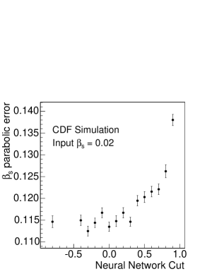
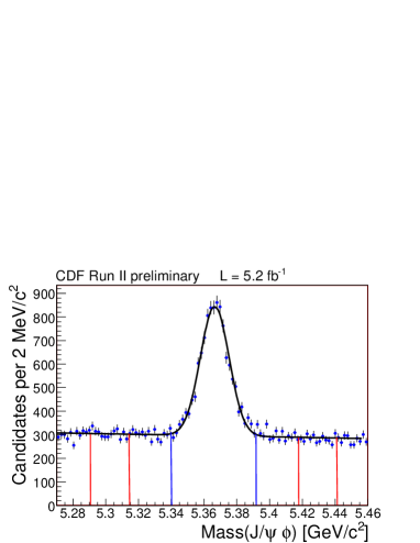
Figure 1: An example of the dependence of parabolic uncertainty of $\beta_{s}^{J\!/\!\psi\phi}$ on ANN output requirement (left). The invariant mass distribution of the selected candidates used in the analysis (right).

In Fig. 1 we show an example of such simulation for true $\beta_{s}^{J\!/\!\psi\phi}$ value at the SM expectation. As result we select candidates with the ANN output larger than 0.2, which is less stringent requirement than one used in previously. The resulting invariant mass distribution contains about 6500 signal events and is shown in Fig. 1.

3 Flavour tagging

The flavour tagging is one of the important tools in the analysis. Its task is to determine whether reconstructed candidate was produced as $B_{s}$ or $\overline{B}_{s}$. Two algorithms are used at hadron colliders. The first one, called opposite side tagging, explores the fact that $b$-quarks are dominantly produced in $b\overline{b}$ pairs, so determination of the flavour of other $b$-hadron determines also the flavour of signal one. The second algorithm, called same side tagging, explores properties of hadrons produced in hadronization of $b$ quark into $B_{s}$ mesons.

The opposite side algorithm explores several sources of information from the non-signal $b$-hadron in an event. The most clean explores the fact that about 10% of $b$-hadrons decay to a final state containing lepton. At CDF we use electrons and muons and given that most of them arise from the $b$-hadron decays in events with reconstructed $B_{s}$, they provide clean information, but at expanse of small efficiency. The second source uses fact the most abundant $b\rightarrow c\rightarrow s$ quark level transition yielding a final state which often contains charged kaon, which determines the flavour of the $b$-hadron. The most efficient source identifies jet containing $b$ quark and calculates weighted charge of the tracks in jet to determine, whether original quark had positive or negative charge and thus determine flavour. While this algorithm is efficient, its purity is rather small. We combine all three sources into single decision using neural network. The quality of decision is predicted for each event and checked on the fully reconstructed $B^{+}$ events. The overall performance of the algorithm is about 1.2%, which can be understood as having 1.2% of the overall statistics with perfectly known production flavour.

The same side algorithm exploits fragmentation process. To form a $B_{s}$ out of $\overline{b}$ quark we need to attach $s$ quark to it. The $s$ quark comes from a pair generated out of the vacuum and after forming $B_{s}$ an $\overline{s}$ quark remains to form other hadron. If it ends up in the charged kaon it can be used to determine the production flavour.

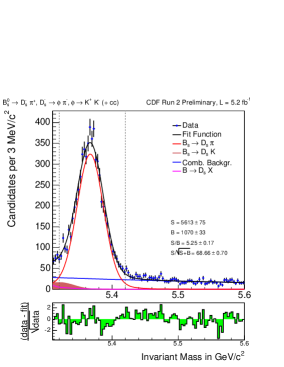
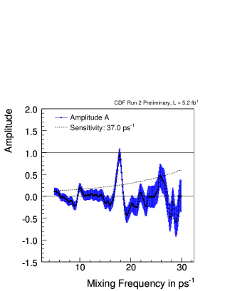
Figure 2: The invariant mass distribution of $B_{s}\rightarrow D_{s}\pi$ with $D_{s}\rightarrow\phi\pi$ (left) and the amplitude scan in the full dataset (right).

The challenge is to identify right kaon in an event with many tracks. Another challenging part is to calibrate quality of the decisions on a data as only process available is $B_{s}$ mixing. Despite all challenges, CDF uses this algorithm with good success. In calibration we use data spanning same period as our dimuon dataset. For calibration we reconstruct about 12900 $B_{s}\rightarrow D_{s}(3)\pi$ signal events. The predicted quality of decision for each event is scaled by a global scaling factor which is determined in the fit for $B_{s}$ oscillations. We show the invariant mass distribution of channel contributing about half of the statistics together with the amplitude scan on full sample in Fig. 2. The resulting tagging performance is about 3.2%. The obtained $B_{s}$ mixing frequency is $\Delta m_{s}=17.79\pm 0.07$ ps^-1 with uncertainty being statistical only. Full details of this calibration can be found in Ref. [5].

4 Fit description

On the limited space available we cannot describe all details of the fit, so we will touch only main features with some emphasis on changes compared to the previous versions of the analysis. The full details are spelled out in Ref. [6]. As spin zero $B_{s}$ decays into two spin one particles ($J\!/\!\psi$ and $\phi$) three different amplitudes corresponding to different angular momentum are involved. In CDF we use a basis in which three amplitudes are written in terms of polarisation amplitudes. The three amplitudes give six angular terms, three terms corresponding to the squares of amplitudes and three corresponding to the interference between amplitudes. Each of the six terms has its own angular and decay time dependence. Some of the terms exhibit usual $\sin(\Delta m_{s}t)$ behaviour and some are proportional to $\cos(\Delta m_{s}t)$. Thanks to the non-zero decay width difference ($\Delta\Gamma$) in the $B_{s}$ system, depending on the size of the $\Delta\Gamma$ and polarisation amplitudes one can gain considerable information on the $CP$ violating phase also without resolving the oscillation pattern.

Since the first analysis there is an ongoing discussion whether there can be contribution from non-resonant $J\!/\!\psi K^{+}K^{-}$ or $J\!/\!\psi f_{0}(980)$ with $f_{0}(980)\rightarrow K^{+}K^{-}$ decays, collectively named s-wave. Those were neglected in previously and there is an open question about the size of possible contribution and whether it can bias result. In the presented result we introduce an s-wave component which is allowed to float during the analysis. This additional component introduces four new terms, one corresponding to the square of the s-wave amplitude and three for the interference between s-wave contribution and decay to $J\!/\!\psi\phi$.

5 Results

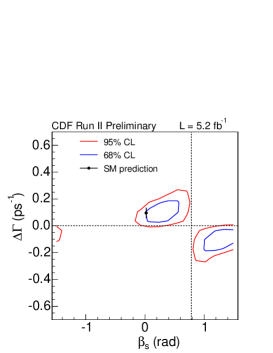
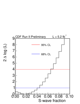
Figure 3: The contours in $\beta_{s}^{J\!/\!\psi\phi}$-$\Delta\Gamma$ plane after full coverage adjustment (left). The likelihood profile for the fraction of s-wave contribution (right).

Similar to the previous iterations, the likelihood in case of all parameters floating still show non-Gaussian behaviour. In order to deal with the likelihood behaviour and ensure well defined statistical meaning of the result we construct confidence regions in the $\beta_{s}^{J\!/\!\psi\phi}$-$\Delta\Gamma$ plane, which are shown in Fig. 3. For the standard model value of $\beta_{s}^{J\!/\!\psi\phi}$ and $\Delta\Gamma$ we obtain the p-value of 44% which corresponds to about 0.8 standard deviations. Minimising also over $\Delta\Gamma$ we obtain the p-value for standard model of 31% with $\beta_{s}^{J\!/\!\psi\phi}\in[0.02,0.52]\cup[1.08,1.55]$ at 68% confidence level and $\beta_{s}^{J\!/\!\psi\phi}\in[-\pi/2,-1.44]\cup[-0.13,0.68]\cup[0.89,\pi/2]$ at 95% confidence level. The amount of s-wave is consistent with zero and the likelihood profile over parameter describing its amount is shown in Fig. 3.

In addition we also perform a fit in which we fix $\beta_{s}^{J\!/\!\psi\phi}=0$. Such configuration provides well behaving likelihood allowing to provide point estimates of several interesting quantities even if the result should be interpreted in the context of standard model. From this fit we measure

$$c\tau = 458.6\pm 7.6(\mathrm{stat})\pm 3.6(\mathrm{syst})\,\mu\mathrm{m},$$

$$\Delta\Gamma = 0.075\pm 0.035(\mathrm{stat})\pm 0.01(\mathrm{syst})\,\mathrm{ps}^{-1},$$

$$|A_{||}|^{2} = 0.231\pm 0.014(\mathrm{stat})\pm 0.015(\mathrm{syst}),$$

$$|A_{0}|^{2} = 0.524\pm 0.013(\mathrm{stat})\pm 0.015(\mathrm{syst}),$$

$$\phi_{\perp} = 2.95\pm 0.64(\mathrm{stat})\pm 0.07(\mathrm{syst}).$$

In all cases, those are the most precise measurements of those quantities up to date. The strong phase $\delta_{||}$ is close to the symmetry point at $\pi$ which makes estimate of its value and uncertainty unreliable and therefore we do not provide result for it.

6 Conclusions

We presented the updated measurement of the $CP$ violating phase $\beta_{s}^{J\!/\!\psi\phi}$ in $B_{s}\rightarrow J\!/\!\psi\phi$ decays from CDF experiment. Using 5.2 $\mathrm{fb^{-1}}$ of data we obtain bounds which are significantly stronger than our previous results. The data itself are consistent with the standard model at 0.8 standard deviation level. The improvement compared to the previous result is better than just simple scaling by the amount of collected data. Few possible improvements are still available in addition to collecting more data. On the data size itself, we expect to double our dataset by the end of 2011 with ongoing discussion for another 3 years extension to Tevatron running.

ACKNOWLEDGEMENTS

The author would like to thank the organisers of the CKM workshop and working group conveners for kind invitation and for providing forum for discussions. Also my CDF colleagues actively pursuing this analysis deserve acknowledgement for their hard work needed to push forward this non-trivial but exciting analysis.

References

- [1] J. H. Christenson et al., Phys. Rev. Lett. 13 (1964) 138.
- [2] M. Kobayashi and T. Maskawa, Prog. Theor. Phys. 49 (1973) 652.
- [3] B. Aubert et al. [B A B AR Collaboration], Phys. Rev. Lett. 86 (2001) 2515; K. Abe et al. [Belle Collaboration], Phys. Rev. Lett. 87 (2001) 091802.
- [4] T. Aaltonen et al. [CDF Collaboration], Phys. Rev. Lett. 100 (2008) 161802; V. M. Abazov et al. [ D0 Collaboration ], Phys. Rev. Lett. 101 (2008) 241801.
- [5] The CDF Collaboration, CDF Public Notes 10206 and 10108.
- [6] F. Azfar et al., [arXiv:1008.4283 [hep-ph]].