Homogeneous photospheric parameters and C abundances
in G and K nearby stars with and without planets ^,

Abstract

Aims. We present a determination of photospheric parameters and carbon abundances for a sample of 172 G and K dwarf, subgiant, and giant stars with and without detected planets in the solar neighbourhood. The analysis was based on high signal-to-noise ratio and high resolution spectra observed with the ELODIE spectrograph (Haute Provence Observatory, France) and for which the observational data was publicly available. We intend to contribute precise and homogeneous C abundances in studies that compare the behaviour of light elements in stars, hosting planets or not. This will bring new arguments to the discussion of possible anomalies that have been suggested and will contribute to a better understanding of different planetary formation process.

Methods. The photospheric parameters were computed through the excitation potential, equivalent widths, and ionisation equilibrium of iron lines selected in the spectra. Carbon abundances were derived from spectral synthesis applied to prominent molecular head bands of ${\rm C}_{2}$ Swan ($\lambda$5128 and $\lambda$5165) and to a C atomic line ($\lambda$5380.3). Careful attention was drawn to carry out such a homogeneous procedure and to compute the internal uncertainties.

Results. The distribution of [C/Fe] as a function of [Fe/H] shows no difference in the behaviour of planet-host stars in comparison with stars for which no planet was detected, for both dwarf and giant subsamples. This result is in agreement with the hypothesis of primordial origin for the chemical abundances presently observed instead of self-enrichment during the planetary system formation and evolution. Additionally, giant stars are clearly depleted in [C/Fe] (by about 0.14 dex) when compared with dwarfs, which is probably related to evolution-induced mixing of H-burning products in the envelope of evolved stars. Subgiant stars, although in small number, seems to follow the same C abundance distribution as dwarfs. We also analysed the kinematics of the sample stars that, in majority, are members of the Galaxy’s thin disc. Finally, comparisons with other analogue studies were performed and, within the uncertainties, showed good agreement.

1 Introduction

The Sun was usually assumed to be formed from the material representative of local physical conditions in the Galaxy at the time of its formation and, therefore, to represent a standard chemical composition. However, this homogeneity hypothesis has been often put in question as a consequence of many improvements in the observations techniques and data analysis. With the discovery of extrasolar planetary systems, the study of heterogeneity sources (e.g. stellar formation process, stellar nucleosynthesis and evolution, collisions with molecular clouds, radial migration of stars in the Galactic disc) has gained a new perspective and brought new questions.

It is now a fact that dwarf stars hosting giant planets are, on average, richer in metal content than stars in the solar neighbourhood for which no planet has been detected (see e.g. Fischer & Valenti 2005; Gonzalez 2006; Santos et al. 2001, 2004). Two hypotheses have been suggested trying to explain the origin of this anomaly: i) primordial hypothesis: the chemical abundances presently observed would represent those of the protostellar cloud from which the star was formed; ii) self-enrichment hypothesis: a significant amount of material enriched in metals would be accreted by the star during the planetary system formation and evolution.

It has been speculated that abundance anomalies between dwarf stars with and without planets may not only involve the metal content of heavy elements but also the abundance of light elements, like carbon and oxygen, measured by an overabundance in the ratio [X/Fe] of one stellar group in spite to the other, in a given metallicity range. Gonzalez & Laws (2000) found that [Na/Fe] and [C/Fe] in stars with planets are, on average, smaller than in stars with no detected planets, for the same metallicity. Numerical simulations performed by Robinson et al. (2006) predicted an overabundance of [O/Fe] in planet-host stars. The same result for this element was obtained by Ecuvillon et al. (2006), although the authors noticed that it is not clear if this difference is due to the presence of planets.

In other publications, however, no difference was found in the abundance ratios of light elements when comparing stars with and without planets (Ecuvillon et al. 2004a, b; Luck & Heiter 2006; Takeda & Honda 2005). In particular, in more recent studies, Gonzalez & Laws (2007) and Bond et al. (2008) do not confirm the overabundance of [O/Fe] in planet-host stars obtained by Ecuvillon et al. (2006) and Robinson et al. (2006), showing that a solution for the problem is not simple.

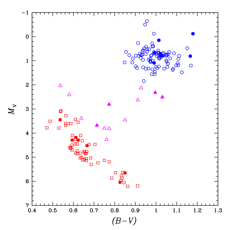
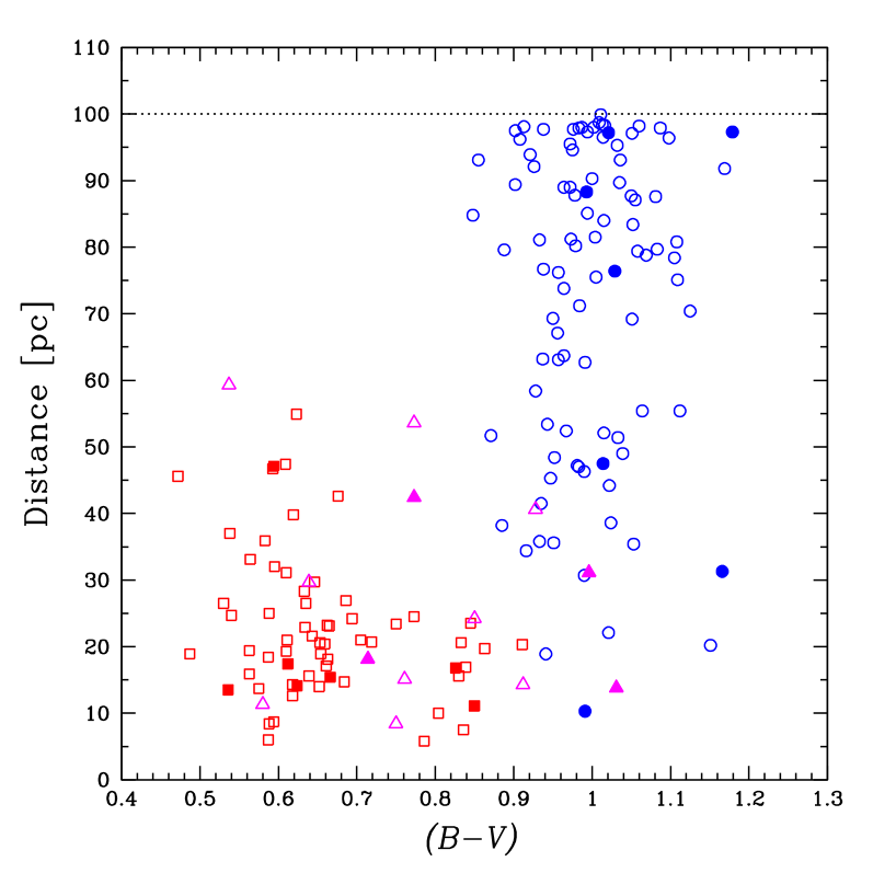
Figure 1: HR (left panel) and colour-distance (right panel) diagrams for 63 dwarfs ( $\square$), 13 subgiants ( $\triangle$), and 96 giants ( $\circ$) analysed in this work. Filled symbols represent stars with detected planets. The distance limit of 100 pc is also shown (dotted line).

Most of the studies above are not conclusive and the discussion about this problem remains open. New tests are encouraged, using more precise and homogeneous data, with a number of stars as large as possible. In the present work we show the results of our analysis of high quality spectra, in which we determined photospheric parameters and carbon abundances for 172 G and K stars, including 18 planet hosts. Although this kind of investigation is not new, the spectra analysed here offer the possibility to perform an homogeneous and accurate study of the chemical anomalies that have been proposed in the literature and will surely help to distinguish the different stellar and planetary formation processes.

The abundance distribution of light elements in stars more evolved than the Sun, hosting planets or not, have also been studied. Takeda et al. (2008) analysed a large sample of late-G giants, including a few stars hosting planets. For a solar metallicity, the authors found an underabundance of [C/Fe] and [O/Fe] as well as an overabundance of [Na/Fe] in the atmosphere of their sample stars compared to previous results for dwarf stars, which they attributed to evolution-induced mixing of H-burning products in the envelope of evolved stars.

Our sample comprises 63 dwarf stars (from which 7 have planets), 13 subgiants (4 with planets), and 96 giants (7 with planets). This allowed us to investigate possible anomalies in the abundance ratios of stars more evolved than the Sun. Excepting HD 7924, whose planet has a minimum mass of 9 Earth masses (about half that of Neptune), the planet-host stars in question come from systems that have at least one giant planet.

The data and the reduction process are presented in Sect. 2. The determination of the photospheric parameters and their uncertainties are described in Sect. 3. In Sect. 4 we describe the spectral synthesis method used to obtain the carbon abundances and their uncertainties. Our results are presented and discussed in Sect. 5, and final remarks and conclusions done in Sect. 6.

2 Observation data and reduction

Our sample consists of 172 G and K dwarf, subgiant, and giant stars in the solar neighbourhood (distance $<$ 100 pc) observed with the ELODIE high-resolution échelle spectrograph (Baranne et al. 1996) of the Haute Provence Observatory (France). The analysis was done based on spectra that were publicly available in the ELODIE archive (Moultaka et al. 2004) when the work started. The spectra have resolution $R=42\,000$ and cover the wavelength range 3895$-$6815 Å. The resulting sample stars were selected according to the following criteria:

• stars for which the averaged spectra have S/N $\geq$ 200; among all individual spectra available in the database, only those having S/N $\geq$ 30 and with an image type classified as object fibre only (OBJO) were used;

• stars within a distance $\leq$ 100 pc (parallax $\pi\geq$ 10 mas) and with spectral type between F8 and M1; earlier type stars have a small number of spectral lines whereas dwarfs later than M1 are quite faint to provide good quality spectra, and also quite cold (exhibiting a lot of strong molecular features, such as the TiO bands), making difficult the determination of precise abundances;

• stars for which no close binary companion is known, since these objects may contaminate the observed spectra; we used the information of angular separation between components ($rho$) available in the Hipparcos catalogue (ESA 1997), choosing only the cases with $rho>$ 10 arcsec.

• stars for which the determination of the photospheric parameters (Sect. 3) is reliable;

• stars with ($B-V$) values measured by Hipparcos and with spectral cross-correlation parameters available in the ELODIE database; both ($B-V$) and the width of the cross-correlation function are required in the estimate of the stellar projected rotation velocity v$\sin{i}$ (see Sect. 4); and

• stars that passed the quality control of the spectral synthesis (see Sect. 4).

The selected sample is plotted in the HR and colour-distance diagrams of Fig. 1, separating the subsamples of dwarfs, subgiants, and giants. The transition boundaries between dwarfs and subgiants and also between subgiants and giants are not clearly defined on an observational HR plane. In this work, we chose to classify as subgiants those stars situated 1.5 mag above the lower limit of the main-sequence and having $M_{\rm v}>2.0$ mag. Note that the distance of dwarfs and subgiants is not limited to 100 pc, but to about 60 pc. This is not an imposition of our selection criteria, but a selection effect of ELODIE observation surveys instead.

For each sample star, the spectra available in the ELODIE database were processed using IRAF  routines. First, they were normalised (a global pre-normalisation) based on continuum windows selected in the wavelength range. Then the normalised spectra were corrected from Doppler effect, i.e., transformed to a rest wavelength scale taking the solar spectrum as reference, with a precision of better than 0.02 Å in the correction. After these two first steps, the spectra were averaged to reduce noise. Finally, a more careful normalisation was done, this time only considering a small wavelength region around the spectral features analysed in this work: for the molecular bands the range 5100$-$5225 Å were used, and for the C atomic line the wavelength range was 5330$-$5430 Å. At this point, the stellar spectra were ready to be used by the synthesis method.

3 Determination of photospheric parameters

A precise and homogeneous determination of chemical abundances in stars depends on the calculation of realistic model atmospheres, which in turn depends on accurate stellar photospheric parameters: the effective temperature $T_{\rm eff}$, the metallicity [Fe/H], the surface gravity $\log{g}$, and the micro-turbulence velocity $\xi$. We developed a code that uses these four parameters as input and, iteratively changing their values, try to find a solution for the model atmosphere and metal abundance that are physically acceptable.

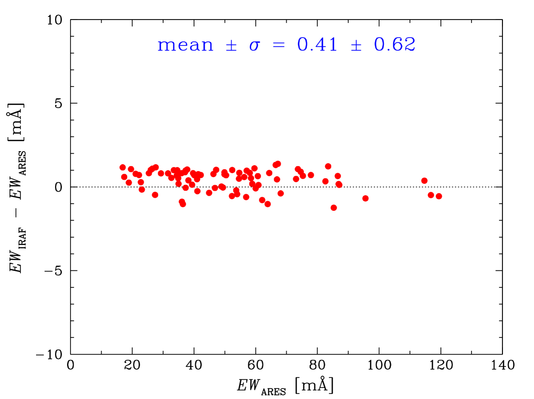
Figure 2: Equivalent widths of Fe i and Fe ii lines in the spectrum of the sunlight reflected by the Moon measured using ARES in comparison to those measured using IRAF tasks.

The abundance yielded by different spectral lines of the same element should not depend on their excitation potential ($\chi$) or their equivalent width ($EW$). Also, neutral and ionised lines of the same element should provide the same abundance as well. Therefore, in this work, the effective temperature was computed through the excitation equilibrium of neutral iron by removing any dependence in the [Fe i/H] $versus$ $\chi$ diagram. Additionally, by removing any dependence of [Fe i/H] on $EW$, the micro-turbulence velocity was estimated. The surface gravity was computed through the ionisation equilibrium between Fe i and Fe ii, and the metallicity was yielded by the $EW$ of Fe i lines. In other words, the photospheric parameters were determined following the conditions below:
— slope([Fe i/H] $versus$ $\chi$) — $<c_{1}$ (dependence on $T_{\rm eff}$) — slope([Fe i/H] $versus$ $EW$) — $<c_{2}$ (dependence on $\xi$) — [Fe i/H] $-$ [Fe ii/H] — $<c_{3}$ (dependence on $\log{g}$) — [Fe/H] $-$ [Fe i/H] — $<c_{4}$
where $c_{1}$, $c_{2}$, $c_{3}$, and $c_{4}$ are arbitrary constants as small as one wishes. If at least one of the first three conditions is not satisfied, then $T_{\rm eff}$, $\xi$, and/or $\log{g}$ are changed by a given step. In the fourth condition, the value of metallicity [Fe/H] used as input is compared to the one provided by Fe i lines and, if this condition is not satisfied, the code defines [Fe/H] = [Fe i/H]. Therefore, the code iteratively executes several cycles until these four conditions are satisfied at the same time.

Atomic line parameters (wavelength, oscillator strength $gf$, and lower-level excitation potential $\chi$) for 72 Fe i and 12 Fe ii lines used in our analysis are listed in Table 1. They were all taken from the Vienna Atomic Line Database – VALD (Kupka et al. 2000, 1999; Piskunov et al. 1995; Ryabchikova et al. 1997), though the $gf$ values were revised to fit the $EW$ measured in the Kurucz Solar Flux Atlas (Kurucz et al. 1984), along with a model atmosphere for $T_{\rm eff}$ = 5777 K, $\log{g}$ = 4.44, $\xi$ = 1.0 km s^-1, and $\log{\epsilon}_{\,\odot}$ = 7.47 (the solar Fe abundance). Concerning the calculations of the van der Waals line damping parameters, we adopted the Unsöld approximation multiplied by 6.3.

The stellar model atmospheres used in the spectroscopic analysis are those interpolated in a grid derived by Kurucz (1993) for stars with $T_{\rm eff}$ from 3500 to 50 000 K, $\log{g}$ from 0.0 to 5.0 dex, and [Fe/H] from $-$5.0 to 1.0 dex. These are plan-parallel and LTE models, computed over 72 layers. For each layer, the quantities column density ($\rho$x), temperature ($T$), gas pressure ($P_{\rm g}$), electronic density ($N_{\rm e}$), and Rosseland mean opacity ($\kappa_{\rm Ross}$) are listed. The models also include the micro-turbulence velocity, the elemental abundances in the format $\log{\epsilon}$ (where $\log{\epsilon}_{\rm\,star}=\log{\epsilon}_{\,\odot}+$ [Fe/H]), both assumed to be constant in all layers, and a list of molecules used in the molecular equilibrium computation. Although the Kurucz models used here were computed for a micro-turbulence velocity $\xi$ = 2 km s^-1, in our iterative computation of the photospheric parameters, $\xi$ was set as a free parameter instead. We believe that this does not significantly affect the chemical analysis performed here, since their uncertainties are dominated by the errors in the other photospheric parameters.

The equivalent widths were measured using the Automatic Routine for line Equivalent widths in stellar Spectra – ARES (Sousa et al. 2007). In order to test the reliability of the automatic measurements, we performed a comparison between $EW$ measured in the solar spectrum (the sunlight reflected by the Moon) using ARES and those measured one by one using IRAF tasks (see Fig. 2). Notice that both procedures provide $EW$ that are consistent with each other within the uncertainties (the absolute differences are smaller than 1.5 mÅ).

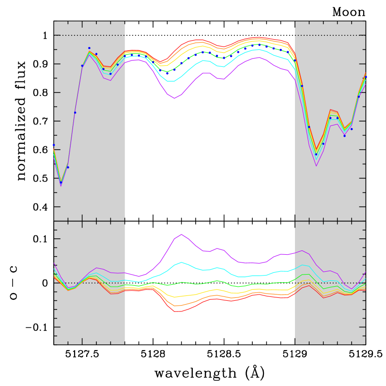
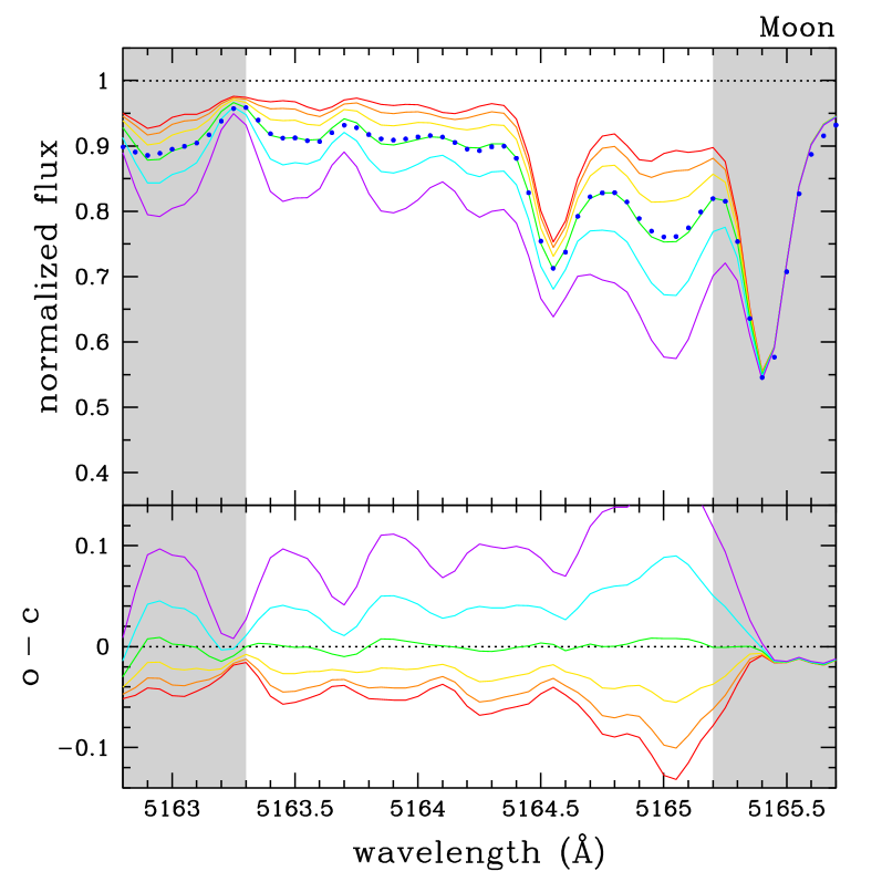
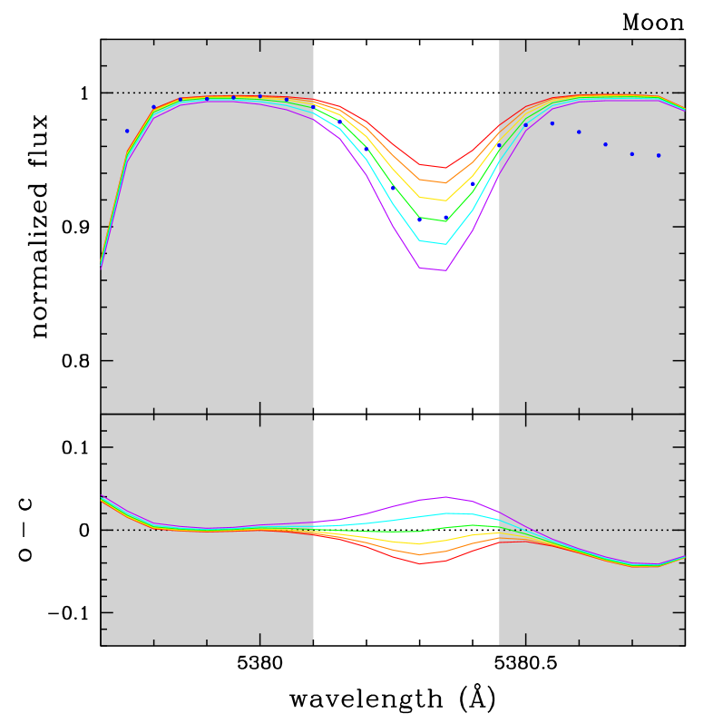
Figure 3: Example to illustrate how the spectral synthesis was applied to observed data (in this case the spectrum of the sunlight reflected by the Moon). The three regions investigated in this work are shown within the hatched areas: the molecular head bands around $\lambda$5128 (left panel) and $\lambda$5165 (middle panel), and the C atomic line at $\lambda$5380.3 (right panel). Six spectra computed for different values of [C/Fe] and distinguished by 0.1 dex are shown. The differences between observed and computed spectra (O$-$C) are also plotted.

3.1 Uncertainties in the photospheric parameters

We developed a routine that iteratively estimates the uncertainties in the computed photospheric parameters of each star. The procedure is as follows:

• first, the micro-turbulence velocity is increased (decreased) by a given step and new model atmospheres are computed; the change proceeds iteratively until the angular coefficient of the linear regression in the [Fe i/H] $versus$ $EW$ diagram is of the same order of its standard error; the absolute differences between increased (decreased) and best values provide the $\xi$ upper (lower) limits; the uncertainty $\sigma(\xi)$ is an average of lower and upper values;

• next, a similar procedure is used for the effective temperature, which is iteratively changed until the angular coefficient of the linear regression in the [Fe i/H] $versus$ $\chi$ diagram is of the same order of its standard error; since micro-turbulence velocity and effective temperature are not independent from each other, the uncertainty $\sigma(\xi)$ estimated above is taken into account before changing $T_{\rm eff}$; thus, the absolute differences between changed and best values of $T_{\rm eff}$ provide the uncertainty $\sigma$($T_{\rm eff}$), with the effect of $\sigma(\xi)$ properly removed;

• the uncertainty in the metallicity $\sigma$([Fe/H]) is the standard deviation of the abundances yielded by individual Fe i lines;

• finally, the uncertainty in the surface gravity $\sigma$($\log{g}$) is estimated by iteratively changing its value until the difference between the iron abundance provided by Fe i and Fe ii is of the same order of $\sigma$([Fe/H]).

4 Carbon abundance from spectral synthesis

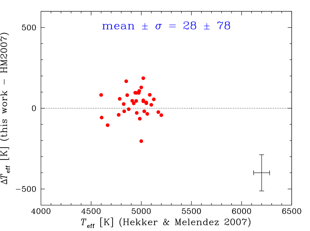
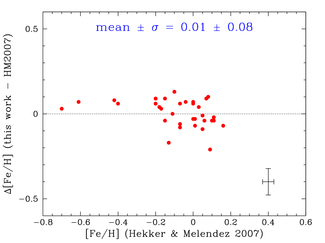
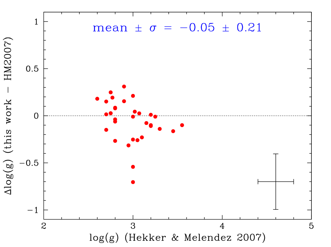
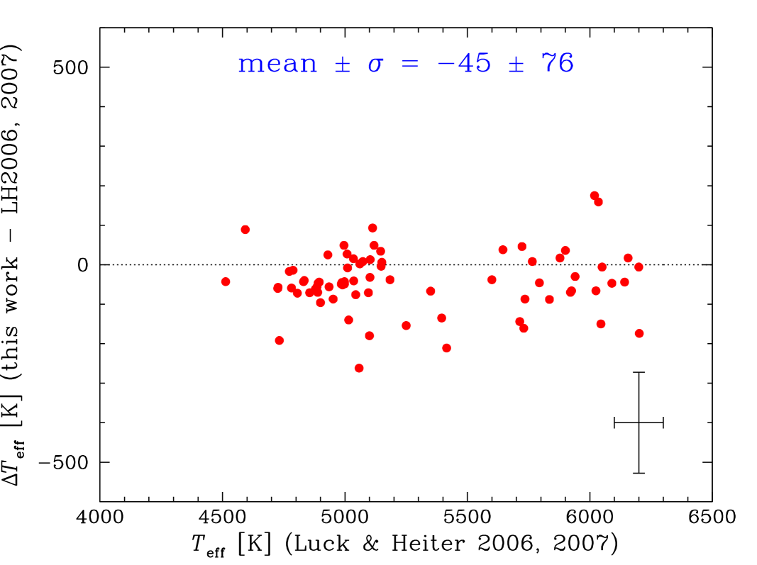
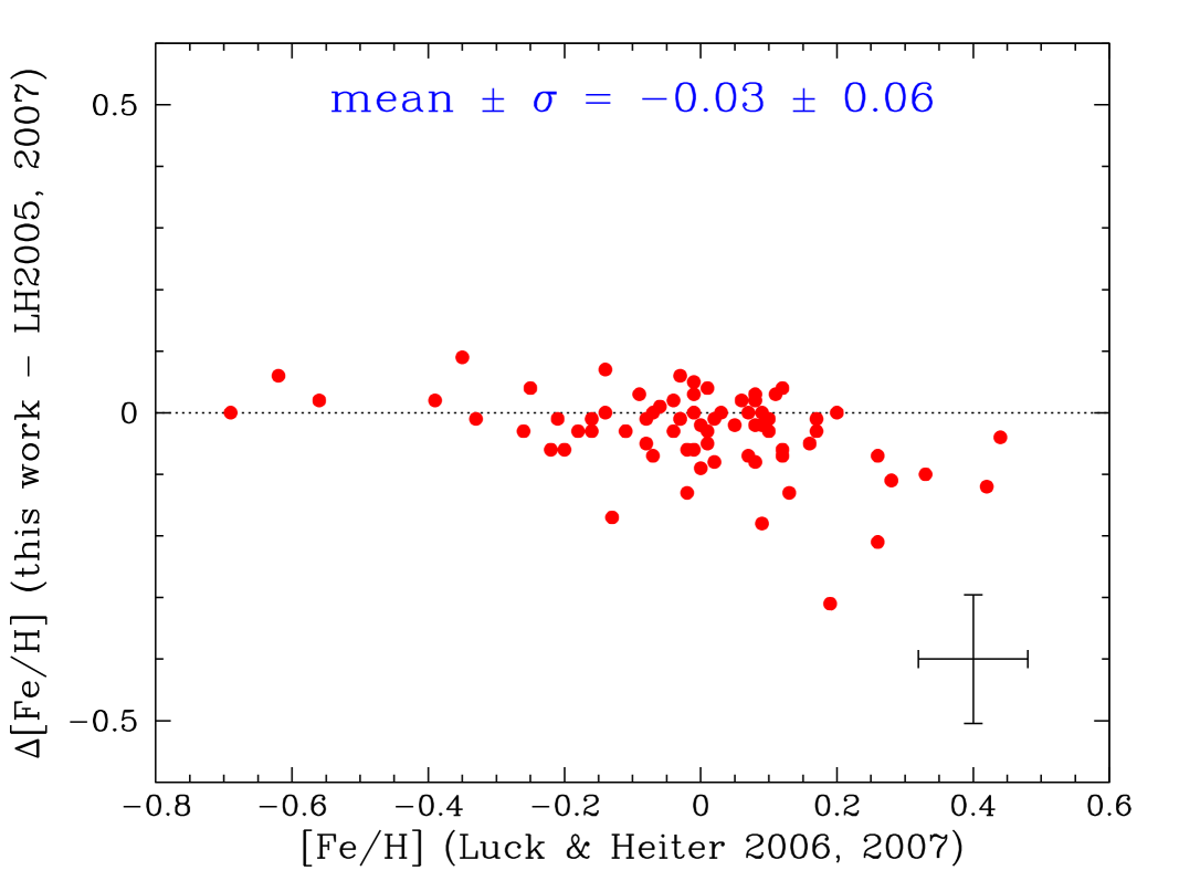
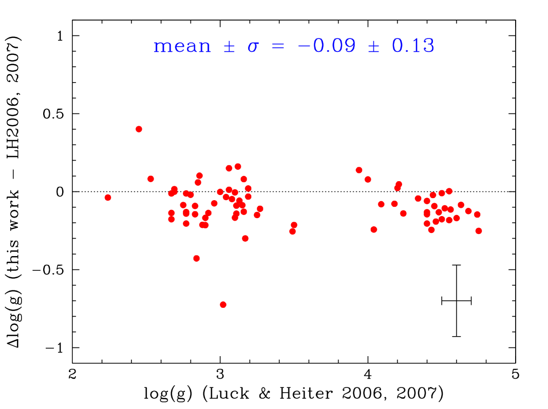
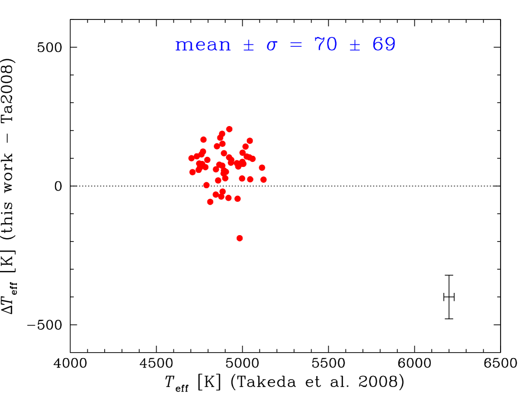
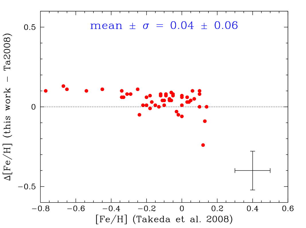
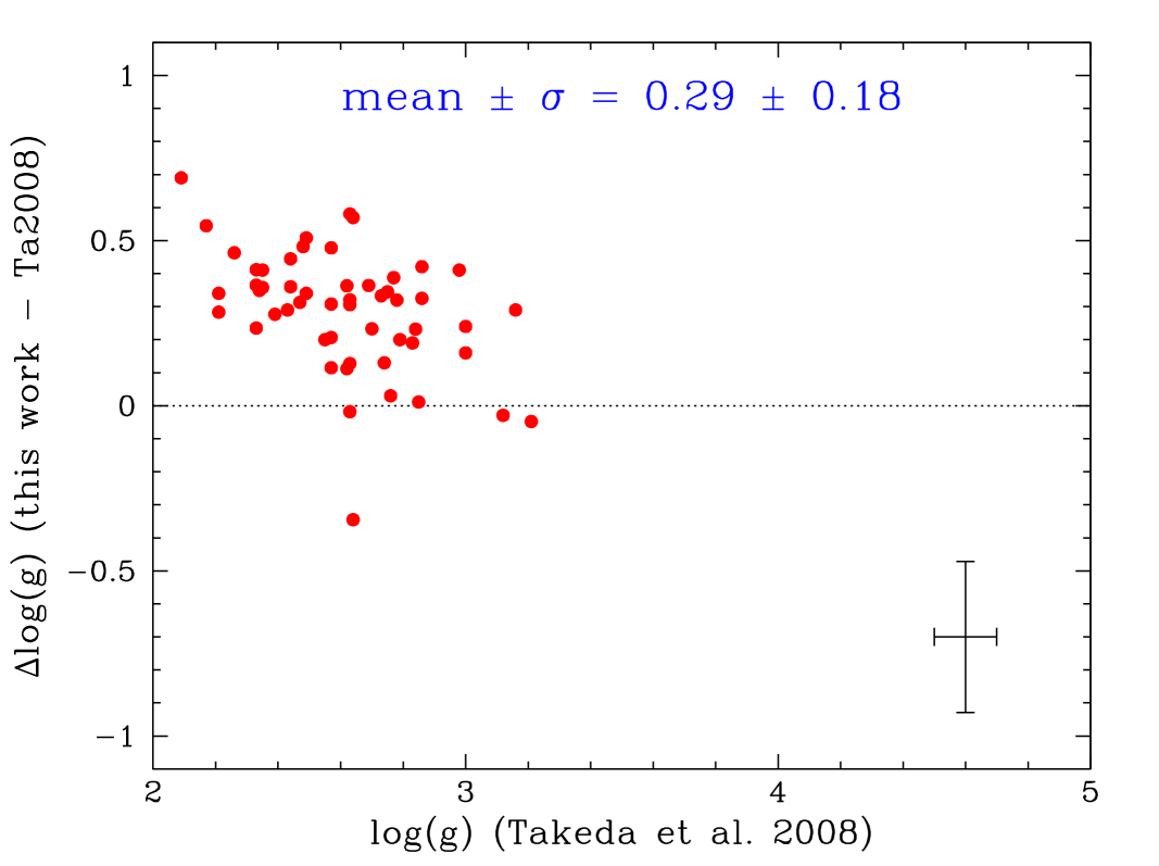
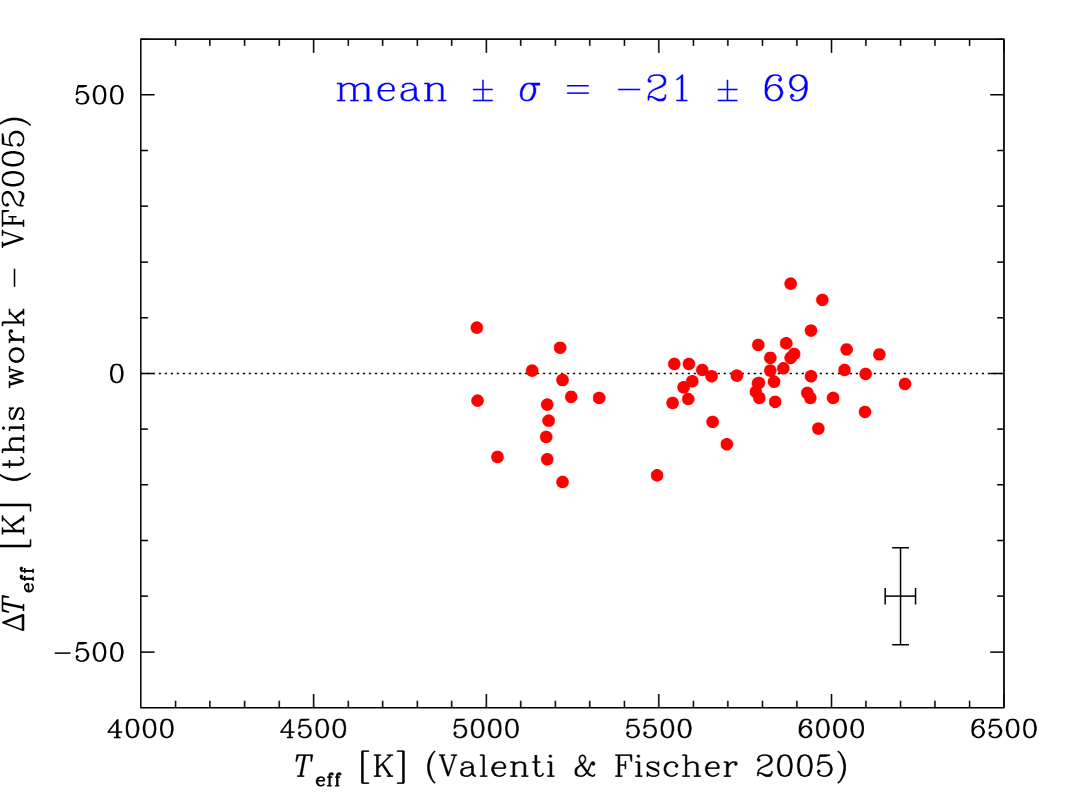
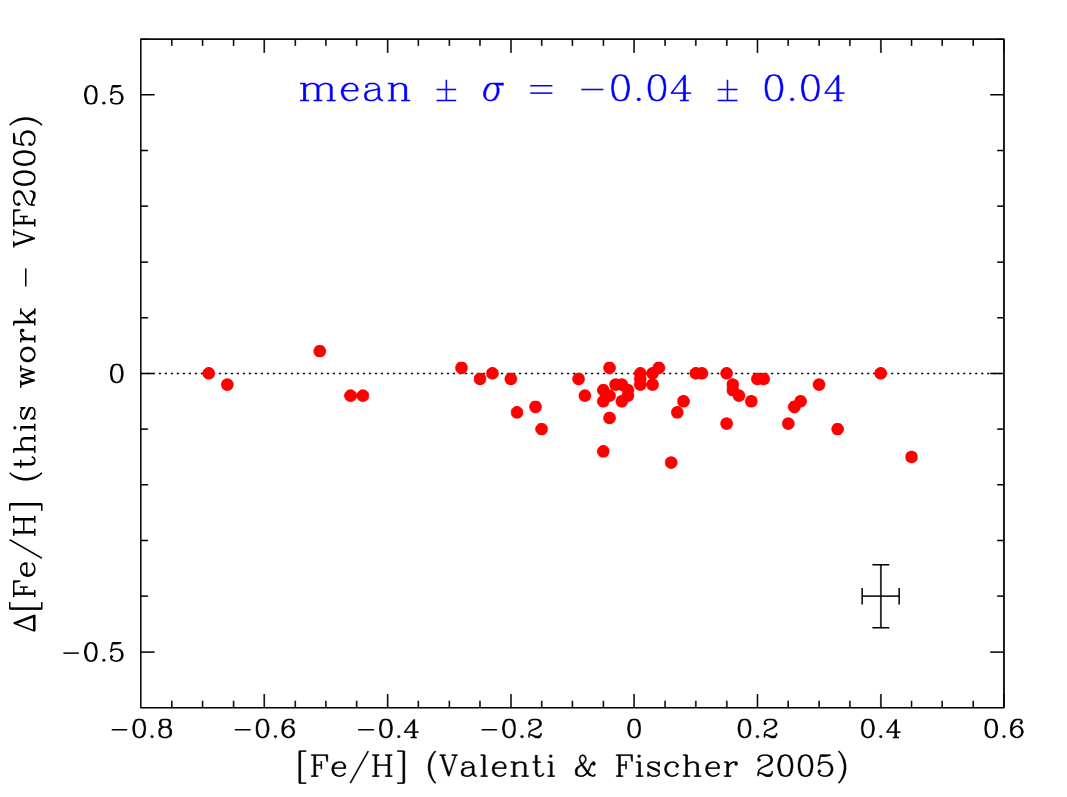
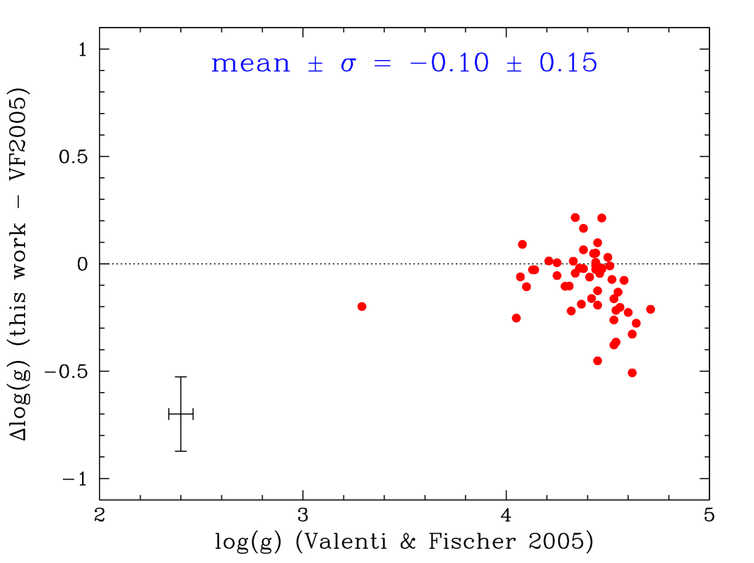
Figure 4: Our determination of effective temperature (left column panels), metallicity (middle column panels), and surface gravity (right column panels) compared to the values published by other works having stars in common. The error bars plotted represent typical uncertainties (see description in the text). The mean value of the differences (this work $-$ comparison paper) and their standard deviations are also shown.

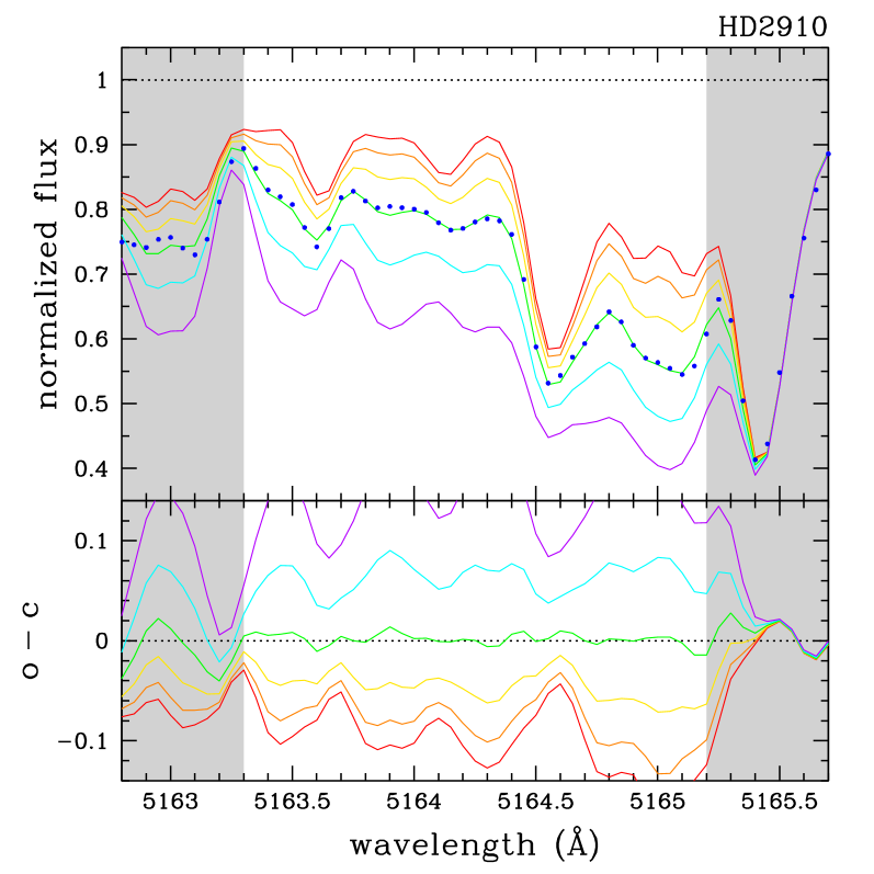
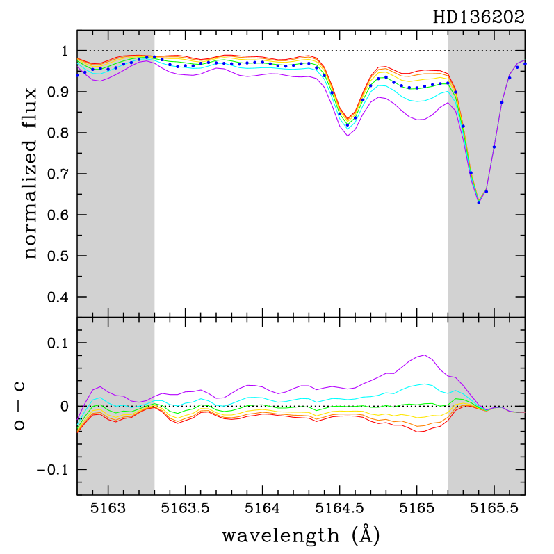
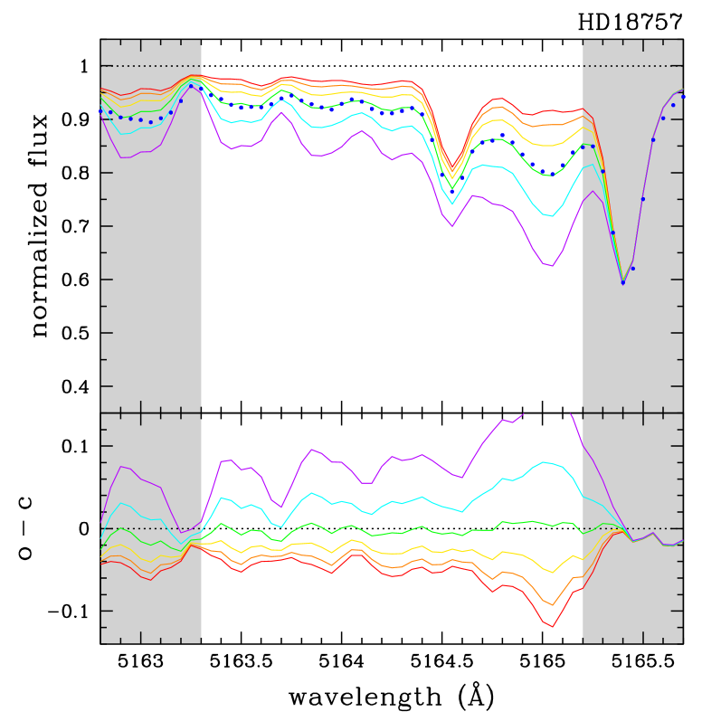
Figure 5: Examples of spectral synthesis applied to different types of stars. Left panel: a cold giant star ($T_{\rm eff}$ = 4815 K), with [Fe/H] and [C/Fe] close to the solar values; Middle panel: a hot dwarf star ($T_{\rm eff}$ = 6215 K), also with solar values for Fe and C abundance; and Right panel: a Fe-poor ([Fe/H] = $-$0.31) dwarf star, for which both temperature and C abundance are close to solar. Other parameters are listed in Tables 4 and 6.

Spectral synthesis was performed to reproduce the observed spectra of the sample stars and thus determine their carbon abundance. The technique was applied to molecular lines of electronic-vibrational head bands of the ${\rm C}_{2}$ Swan System within spectral regions centred at $\lambda$5128 and $\lambda$5165 as well as to a C atomic line at $\lambda$5380.3. The atomic line at $\lambda$5052.2 is also commonly used as a C abundance indicator, but we preferred not to use it since this line is blended with a strong Fe line, which may affect the abundance determination, specially for C-poor stars. Using the MOOG spectral synthesis code (Sneden 2002), synthetic spectra based on atomic and molecular lines were computed in wavelength steps of 0.01 Å, also considering the continuum opacity contribution in ranges of 0.5 Å and line-broadening corrections, and then fitted to the observed spectra.

To compute a theoretical spectrum, the MOOG requires, besides a model atmosphere for each star, some parameters of atomic and molecular spectral lines, which come from the VALD online database and from Kurucz (1995), respectively, and some convolution parameters related to spectral line profiles.

In addition to ${\rm C}_{2}$, another molecule that contributes to the spectral line formation in the studied wavelength regions is MgH, although its contribution is relatively small. The $gf$ of ${\rm C}_{2}$ and MgH lines from the Kurucz database were revised according to the normalisation of the Hönl-London factors (Whiting & Nicholls 1974). The $gf$ values of atomic and other molecular lines were also revised when needed to fit solar spectrum, taken as a reference in our differential chemical analysis.

The parameters of all atomic and molecular lines used to compute the synthetic spectra of the studied regions are listed in Tables 2 and 3, which are only available in electronic form at the CDS. Table 2 contains the following information: the wavelength of the spectral feature, the atomic and molecular line identification, the lower-level excitation potential, the oscillator strength, and the dissociation energy $D_{0}$ (only for molecular features). Table 3 (strong atomic lines) contains the same information of Table 2, excepting the dissociation energy parameter.

The convolution parameters responsible for spectral line broadening that are important to our analysis are: i) the spectroscopic instrumental broadening; ii) a composite of velocity fields, such as rotation velocity and macro-turbulence, that we named $V_{\rm broad}$; and iii) the limb darkening of the stellar disc. We estimated the instrumental broadening by measuring the Full Width at Half Maximum (FWHM) of thorium lines in a Th-Ar spectrum observed with ELODIE. As a first estimate of $V_{\rm broad}$, the projected rotation velocity v$\sin{i}$ of the star was used, which was computed according to Queloz et al. (1998). Then, small corrections in $V_{\rm broad}$ based on an eye-trained inspection of the spectral synthesis fit were applied when needed. Concerning the stellar limb darkening, an estimate of the linear coefficient ($u$) was performed by interpolating $T_{\rm eff}$ and $\log{g}$ in Table 1 of Díaz-Cordovés (1995), and it ranges from 0.63 to 0.83 for the stars in our sample.

Figure 3 shows the spectral synthesis method applied to the observed data. In this illustrative example, the spectrum of the sunlight reflected by the Moon is plotted, showing how reliable is the reproduction of the Sun’s spectrum. Synthetic spectra were computed for the molecular band heads around $\lambda$5128 and $\lambda$5165, and the C atomic line at $\lambda$5380.3, in steps of 0.01 Å, but resampled in steps of 0.05 Å in order to consistently match the observed spectrum wavelength scale.

4.1 Uncertainties in the C abundances

The three wavelength regions investigated in this work provide an independent determination of C abundance and its respective uncertainty. To estimate the uncertainties due to the errors in the photospheric parameters, we developed a routine that takes into account the error propagation of input parameters used by the MOOG spectral synthesis code, namely, $T_{\rm eff}$, $\log{g}$, [Fe/H], $\xi$, and $V_{\rm broad}$. Each one in turn, the MOOG input parameters are iteratively changed by their errors, and new values of the abundance ratio [C/Fe] are computed. The difference between new and best determination provides the uncertainty due to each parameter. The uncertainty $\sigma$([C/Fe]) is a quadratic sum of individual contributions. The error in $V_{\rm broad}$ was estimated to be of the order of 1 km s^-1 or smaller. The error in the limb darkening coefficient was not considered since its contribution can be neglected. In any case, the uncertainty in the C abundances obtained here is dominated by the errors in $T_{\rm eff}$, $\log{g}$, and [Fe/H].

5 Results and discussion

The photospheric parameters and C abundances obtained in the present work, together with their uncertainties, are listed in Tables 4, 5, and 6 for dwarfs, subgiants, and giants, respectively. Table 7, only available in electronic form at the CDS, contains the individual [C/Fe] determinations provided by the three abundance indicators: the star name, the [C/Fe] abundance ratio and its uncertainty yielded by the ${\rm C}_{2}$ molecular band indicator around $\lambda$5128, [C/Fe] and its uncertainty computed from the $\lambda$5165 indicator, and [C/Fe] and its uncertainty computed from the $\lambda$5380.3 indicator.

Both molecular and atomic indicators agree quite well, providing a $rms$ of 0.06 dex in the C abundances. When comparing the two molecular indicators $\lambda$5128 and $\lambda$5165, a $rms$ of only 0.02 dex is found. The fact that the atomic indicator $\lambda$5380.3 is a quite weak line ($EW\sim 20$ mÅ in the Sun’s spectrum) could explain the larger dispersion. Nonetheless, we notice that the final C abundances listed in Tables 4-6 are the result of a weighted average of the abundances yielded by the three C abundance indicators, and that the weights are inversely proportional to the individual uncertainties in each determination.

Figure 4 shows a comparison of the photospheric parameters obtained in this work to those published by other works having stars in common. Effective temperature, metallicity, and surface gravity of dwarf, subgiant, and giant stars are compared with the results of Hekker & Meléndez (2007), Luck & Heiter (2006, 2007), Takeda et al. (2008), and Valenti & Fischer (2005). The errors in the difference this work $-$ comparison paper are a quadratic sum of the errors in our photospheric parameters and those published by the papers. Typical values are represented by error bars plotted in each panel of the figure. The micro-turbulence velocity comparisons are not shown in Fig. 4, but our determination is consistent, within the uncertainties, with the publications above for which an estimate of this parameter was also performed.

The photospheric parameters in the comparison papers are also based on an homogeneous analysis of high signal-to-noise ratio and high resolution data. We can observe in Fig. 4 a very good agreement between our estimates and different determinations. An exception is the surface gravity values of Takeda et al. (2008), which are systematically lower than in our work. The authors also found that their $\log{g}$ determination is systematically lower than in previous studies, whose cause seems to be due to different set of spectral lines used, as they suggested.

For the Sun, our estimate for the photospheric parameters is: $T_{\rm eff}$ = 5724 $\pm$ 38 K, $\log{g}$ = 4.37 $\pm$ 0.10, [Fe/H] = $-$0.03 $\pm$ 0.03, and $\xi$ = 0.87 $\pm$ 0.05 km s^-1. The broadening velocity was set to $V_{\rm broad}$ = 1.8 km s^-1, and the linear limb darkening coefficient, $u$ = 0.69, was obtained in the same way as for the other stars. These values were used to compute the solar model atmosphere, which in turn was used to obtain the solar value of C abundance: [C/Fe] = 0.01 $\pm$ 0.01. Again, as for the other stars, this is the result of a weighted average of the abundances yielded by the three C abundance indicators, where the weights are inversely proportional to the individual uncertainties in each determination.

Figure 5 shows a few examples of spectral synthesis applied to different stars: a cold giant star, a hot dwarf star, and a Fe-poor and high-rotation giant star. The good fit of the synthetic spectra to the observed data in these examples demonstrates that the spectral synthesis method used here provides reliable results for the different spectral types of our stellar sample.

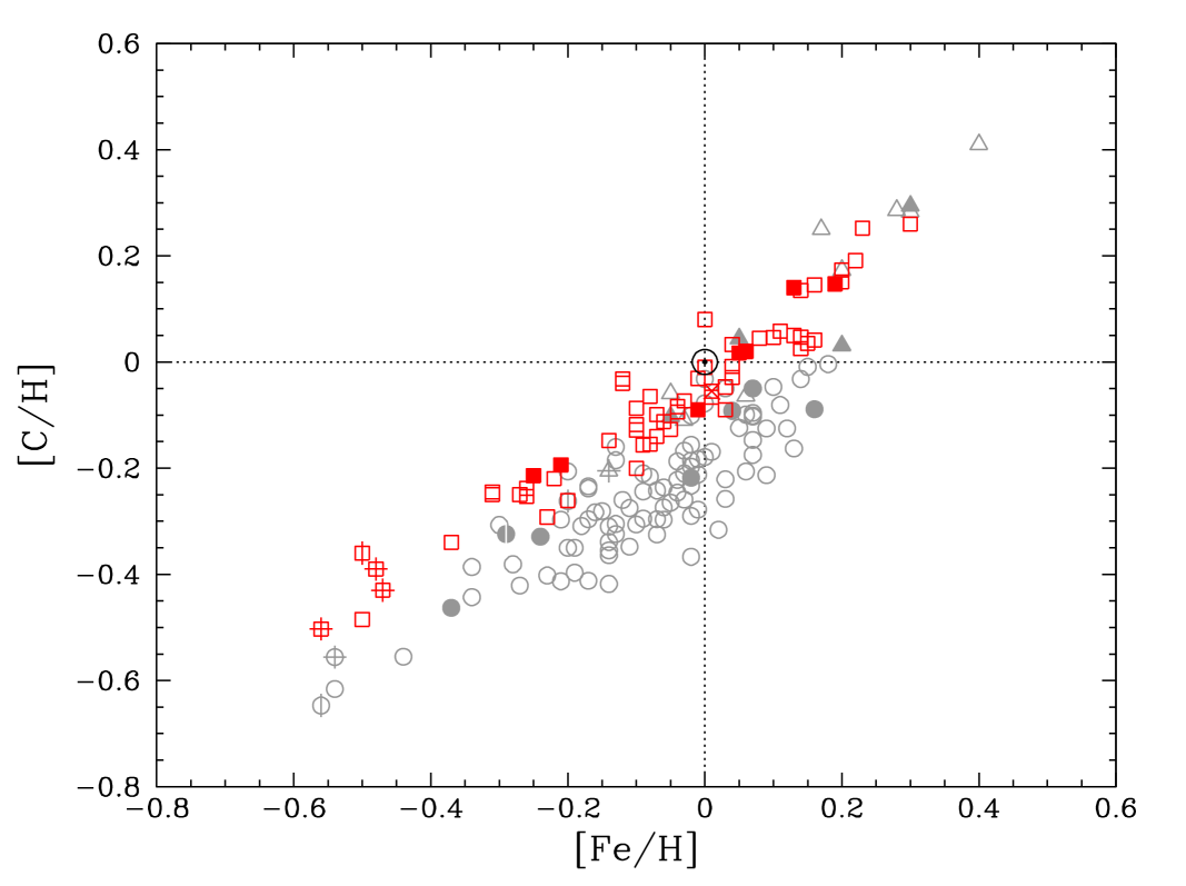
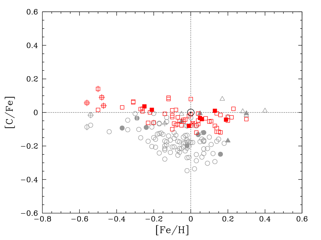
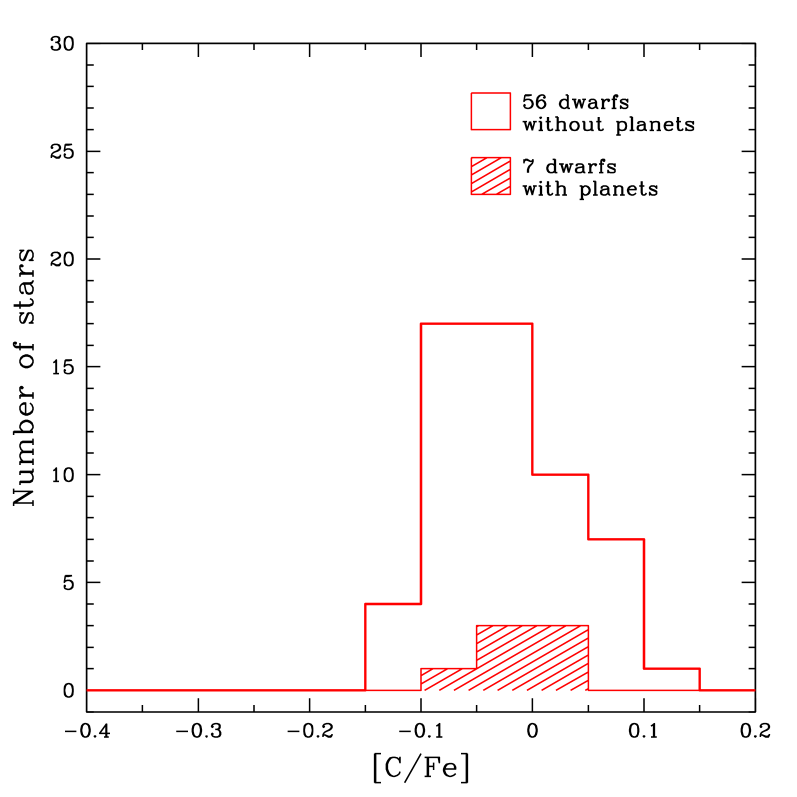
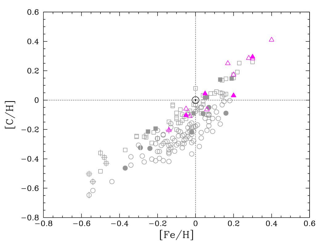
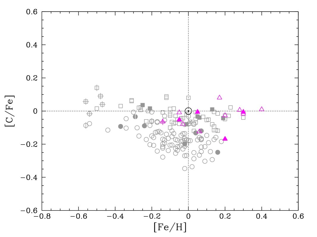
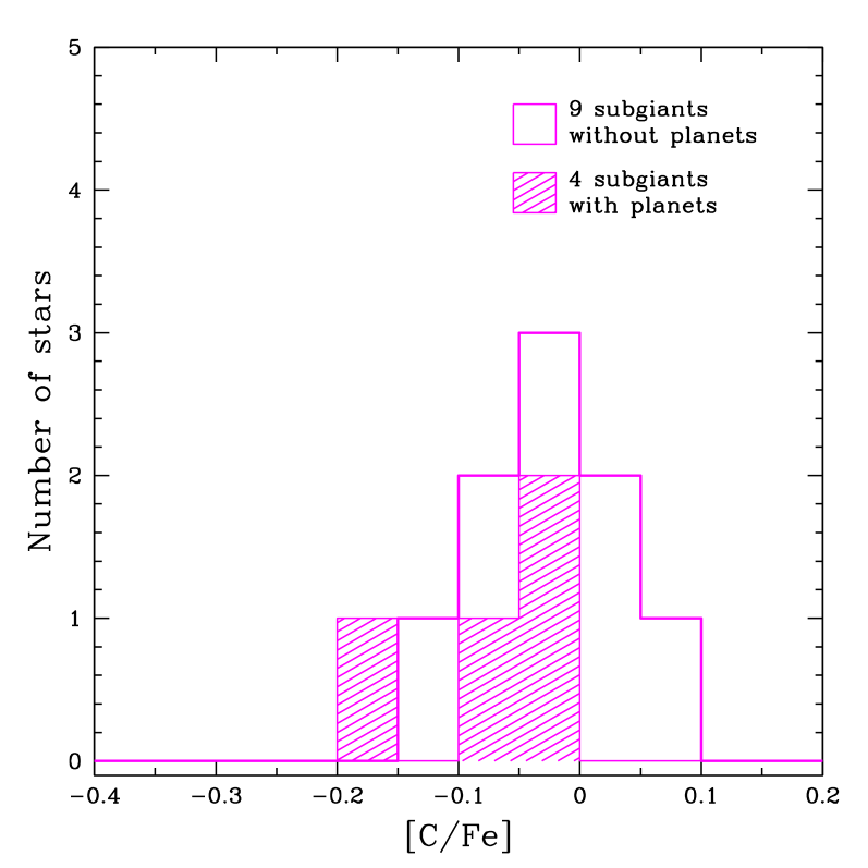
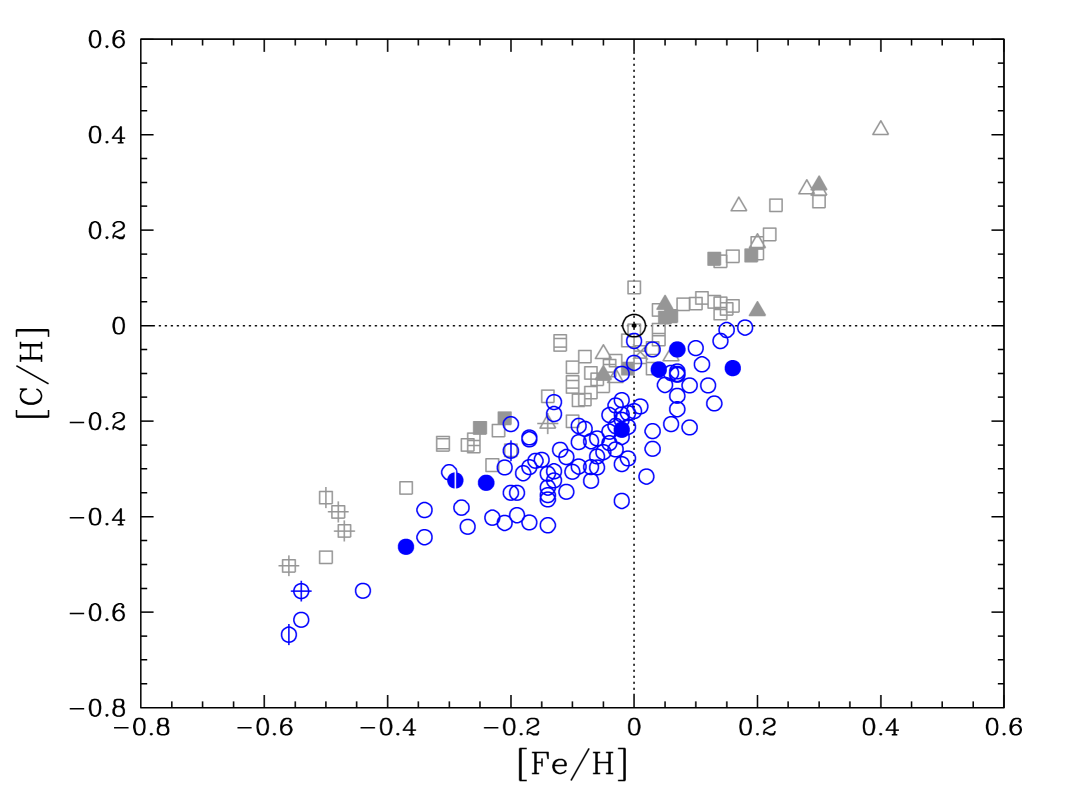
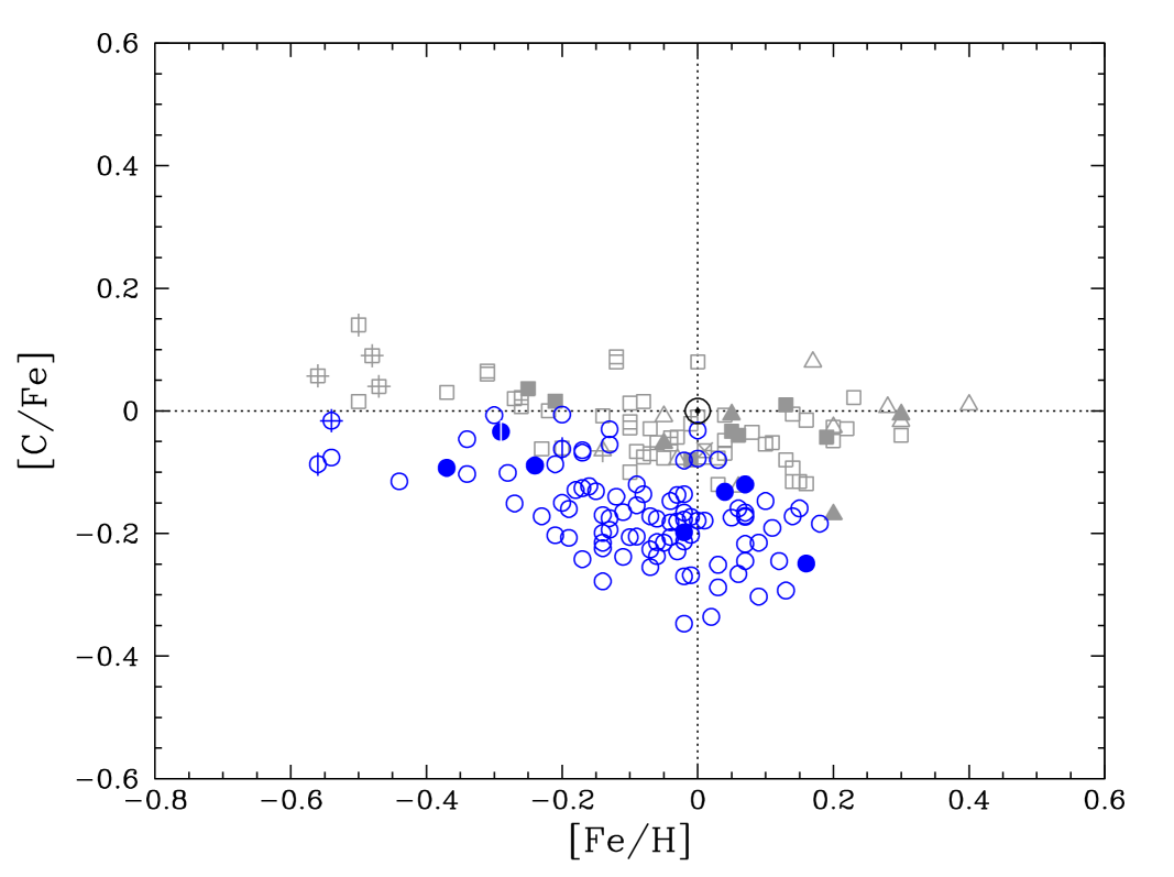
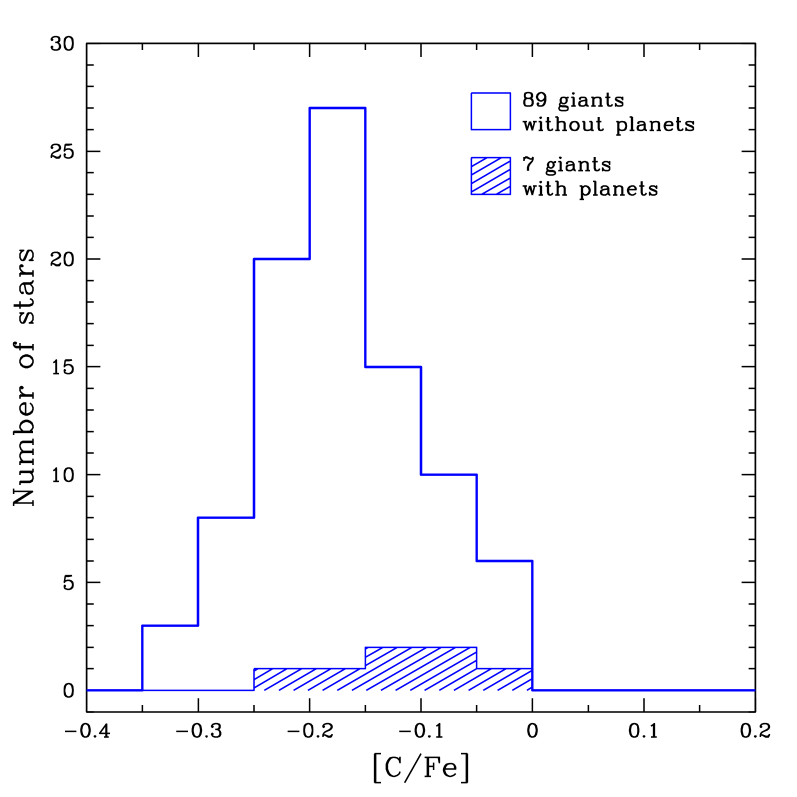
Figure 6: Left and middle column panels: [C/H] and [C/Fe] as a function of [Fe/H] for our sub-samples of dwarfs ( $\square$), subgiants ( $\triangle$), and giants ( $\circ$). Superposed symbols indicate the population classification: thick disc members ($\shortmid$), thin/thick disc (+), and one halo star ($\times$). The remaining stars are thin disc members. Planet hosts are represented by filled symbols. The Sun’s position is also indicated. Each panel focus on one sub-sample, and the two others are shown in light gray. Right column panels: [C/Fe] distributions comparing stars with and without planets.

Figure 6 shows our results of carbon abundance plotted in the form of abundance ratios: [C/H] and [C/Fe] in function of metallicity, and [C/Fe] distributions. Both diagrams and histograms compare the C abundance of planet-host stars with the abundance of stars for which no planet has been detected. To clarify visualisation and simplify the discussion, the three subsamples are presented separately: dwarfs on the top panels, subgiants on the middle panels, and giants on the bottom panels. Choosing a metallicity range in which both stars hosting planets or not are equally represented ($-$0.4 $<$ [Fe/H] $<$ 0.4) and computing the [C/Fe] mean and standard deviation, we have: $i)$ $-0.02\pm 0.04$ and $-0.03\pm 0.05$ respectively for dwarfs with and without planets; $ii)$ $-0.06\pm 0.07$ and $-0.03\pm 0.05$ respectively for subgiants with and without planets; and $iii)$ $-0.13\pm 0.07$ and $-0.17\pm 0.07$ respectively for giants with and without planets. Although it seems that planet-host giants are, on average, richer in [C/Fe] than giants without planets (especially regarding the histogram), according to these values, there is no indication that, in all subsamples, stars with and without planets share different C abundance ratios. In addition, applying a t-test for unequal sample sizes and equal variance, we obtain that the [C/Fe] distributions are indistinguishable with respect to the presence or the absence of planets. These results support the primordial hypothesis discussed in Sect. 1 instead of self-enrichment.

Figure 6 also shows that [C/Fe] is clearly depleted (by about 0.14 dex) in the atmosphere of giants in comparison with dwarf stars. This is in agreement with the results of Takeda et al. (2008) and Liu et al. (2010), which they attributed to evolution-induced mixing of H-burning products in the envelope of evolved stars in the sense that carbon-deficient material, produced by the CN-cycle, would be dredged up to the stellar photosphere.

Our [C/Fe] determinations for dwarfs are somewhat lower than in other works (Ecuvillon et al. 2004b; Gonzalez & Laws 2000; Reddy et al. 2003). We found that the Sun is slightly overabundant in carbon than other dwarfs in the same metallicity range, which is the opposite situation found by those authors. Luck & Heiter (2006, 2007) analysed a large sample of stars also using the spectral synthesis method in the determination of C abundances. In our study we have several stars in common with their papers, and a comparison is shown in Fig. 7. A systematic difference can be observed: our C determination passes from overabundant to underabundant with increasing [C/Fe], at least for dwarfs and giants. We notice, however, that the differences stand mostly from $-0.1$ to $+0.1$ dex, and are compatible with typical uncertainties.

On the other hand, other recent studies corroborate our results in the sense that the Sun seems to be overabundant in carbon with respect to other solar metallicity dwarfs (Ramírez et al. 2009). We have only 5 stars in common with this work, and they are also shown in Fig. 7. In addition, Fig. 1 in their paper for the [C/Fe] abundance ratio is very similar to Fig. 6 for the [C/Fe] distribution of dwarfs in this paper.

It is not unexpected if systematic differences are found between samples analysed by different methods: different model atmospheres, or different set of atomic and molecular lines could produce offsets and trends with respect to other works. Here, stars with planets were compared with their analogues without planets, and dwarfs and subgiants were compared with giants, and they were all analysed using the same method. Therefore, any possible offset that may exist among different works will not affect the analysis of our differential comparison among these subsamples, either the conclusions that we draw.

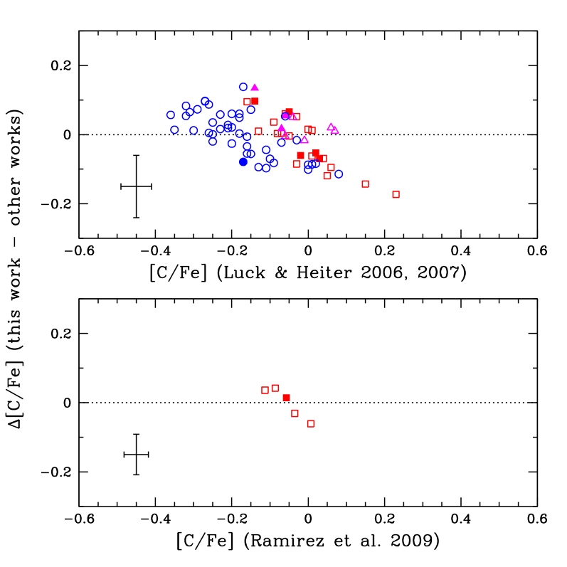
Figure 7: [C/Fe] determination form this study compared to the results of other works having stars in common. The error bars plotted represent typical uncertainties. Symbols are the same as in Fig. 6.

5.1 Kinematics properties

Kinematic properties of the entire sample was considered to investigate the Galaxy population membership. Computation of the kinematics required astrometry (parallaxes and proper motions) and radial velocities. The astrometry was taken from the new reduction of the Hipparcos catalogue (van Leeuwen 2007) and the values of radial velocities were measured from the spectra. The space velocities ($U$, $V$, and $W$) were computed with respect to the local standard of rest (LSR), where the solar motion ($U$, $V$, $W$) = (10.0, 5.3, 7.2) km s^-1 was adopted (see Dehnen & Binney 1998).

With the kinematic data, we have grouped the entire sample into three main populations: thin disc, thick disc, and halo. The probability that a given star in the sample belongs to one of the three populations is computed based on the procedure outlined in Reddy et al. (2006) and references therein. A star whose probability $P_{\rm thin}$, $P_{\rm thick}$, or $P_{\rm halo}$ is greater than or equal to 75% is considered as thin, thick, or halo star, respectively. If the probabilities are in-between, they are considered as either thin/thick disc or thick/halo stars. Out of 172 stars in the sample, vast majority (162) are of the thin disc population and a few metal-poor stars are of the thick disc (just 4). HD 10780 is the only halo star in the sample. With the exception of one thick disc giant, all planet hosts in our sample are thin disc members. Population groups are indicated in Tables 4-6 and also in Fig. 6. The C abundance results seem to be indistinguishable among the different populations.

6 Conclusions

The results presented here represent an homogeneous determination of photospheric parameters and carbon abundances for a large number of G and K stars, comprising 63 dwarfs, 13 subgiants, and 96 giants, from which 18 have already had at least one detected planetary companion at the time of developing this work (mostly giant planets indeed). Our analysis used high signal-to-noise ratio and high-resolution spectra that are public available in the ELODIE online database. We derived the photospheric parameters through the excitation potential, equivalent widths, and ionisation equilibrium of iron lines selected in the spectra. In order to compute the C abundances, we performed spectral synthesis applied to two ${\rm C}_{2}$ molecular head bands ($\lambda$5128 and $\lambda$5165) and one C atomic line ($\lambda$5380.3).

The photospheric parameters here estimated ($T_{\rm eff}$, $\log{g}$, [Fe/H], and $\xi$) are in very good agreement with several works that have stars in common with our sample. These comparison samples were also analysed based on high signal-to-noise ratio and high-resolution data. Our estimates are the result of a precise and homogeneous study, both required conditions to compute reliable model atmospheres used in abundance determinations. Concerning the C abundances, our results point out that:

• regarding the subsamples of dwarfs, subgiants, and giants, there is no clear indication that stars with and without planets have different [C/Fe] or [C/H] abundance distributions;

• [C/Fe] is clearly underabundant (by about 0.14 dex) in the atmosphere of giants in comparison with dwarf stars, which is probably the result of carbon-deficient material, produced by the CN-cycle, dredged-up to the envelope of evolved stars; subgiant stars, although in small number, seem to follow the same behaviour of dwarfs; and

• the Sun is slightly overabundant in carbon in comparison to other dwarf stars with the same metallicity.

The first of the results above are based on small-number statistics. In order to draw more reliable conclusions, a larger number of planet-host stars is required, covering a metallicity range as large as possible. Adding more elements to the study, e.g. nitrogen, oxygen, and some refractory metals, would also expand the analysis to a larger context. In fact, the investigation of volatile and refractory elements with respect to the distribution of their abundances in function of the condensation temperature ($T_{\rm C}$) will shed light on recent controversies aroused by Chavero et al. (2010). The flat distribution found by these authors should be confirmed with more precise abundance determination for $T_{\rm C}\lesssim 300$ K (which includes C, N, and O).

The systematic differences in [C/Fe] found between this and other works are probably related to different analysis method employed to compute the abundances: model atmospheres, the atomic and molecular lines used, etc. Nevertheless, this will not affect our main results since they were based on differential comparisons among subsamples analysed with the same approach.

In this work, we also considered the kinematic properties of our sample to investigate C abundances among different population groups. The stars were separated according to their Galaxy population membership: thin disc, thick disc, or halo stars. We found that most of these stars are members of the thin disc. Moreover, excepting one thick disc star, all planet-host stars are thin disc members. This is probably related either to the fact that giant planets are normally not much detected in less metal-rich stars (the thick disc members indeed) or to the fact that the observation samples are usually limited in distance, which naturally selects thin disc stars.

Table 1: Atomic parameters and solar equivalent widths for 72 Fe i and 12 Fe ii lines used. The equivalent widths listed are those measured (using ARES) in the solar spectrum of the sunlight reflected by the Moon.

$\lambda$ [Å]	ident.	$\chi$ [eV]	$\log{gf}$	$EW_{\odot}$ [mÅ]			$\lambda$ [Å]	ident.	$\chi$ [eV]	$\log{gf}$	$EW_{\odot}$ [mÅ]
4080.88	Fe i	3.65	$-$1.543	58.5			5983.69	Fe i	4.55	$-$0.719	66.5
5247.06	Fe i	0.09	$-$4.932	68.1			5984.82	Fe i	4.73	$-$0.335	83.5
5322.05	Fe i	2.28	$-$2.896	62.1			6024.06	Fe i	4.55	$-$0.124	114.7
5501.48	Fe i	0.96	$-$3.053	116.8			6027.06	Fe i	4.08	$-$1.180	64.4
5522.45	Fe i	4.21	$-$1.419	44.9			6056.01	Fe i	4.73	$-$0.498	73.1
5543.94	Fe i	4.22	$-$1.070	63.9			6065.49	Fe i	2.61	$-$1.616	119.4
5546.51	Fe i	4.37	$-$1.124	54.0			6079.01	Fe i	4.65	$-$1.009	46.3
5560.22	Fe i	4.43	$-$1.064	52.3			6082.72	Fe i	2.22	$-$3.566	34.6
5587.58	Fe i	4.14	$-$1.656	36.4			6089.57	Fe i	5.02	$-$0.883	35.0
5618.64	Fe i	4.21	$-$1.298	49.4			6094.38	Fe i	4.65	$-$1.566	19.6
5619.60	Fe i	4.39	$-$1.435	34.4			6096.67	Fe i	3.98	$-$1.776	37.3
5633.95	Fe i	4.99	$-$0.385	67.2			6151.62	Fe i	2.18	$-$3.296	49.9
5635.83	Fe i	4.26	$-$1.556	32.7			6157.73	Fe i	4.07	$-$1.240	60.7
5638.27	Fe i	4.22	$-$0.809	77.9			6165.36	Fe i	4.14	$-$1.503	41.4
5641.44	Fe i	4.26	$-$0.969	66.9			6180.21	Fe i	2.73	$-$2.636	60.0
5649.99	Fe i	5.10	$-$0.785	36.1			6188.00	Fe i	3.94	$-$1.631	47.2
5651.47	Fe i	4.47	$-$1.763	18.9			6200.32	Fe i	2.61	$-$2.395	73.7
5652.32	Fe i	4.26	$-$1.751	27.4			6226.74	Fe i	3.88	$-$2.066	26.5
5653.87	Fe i	4.39	$-$1.402	37.8			6229.24	Fe i	2.84	$-$2.893	39.7
5661.35	Fe i	4.28	$-$1.828	23.1			6240.65	Fe i	2.22	$-$3.294	49.9
5662.52	Fe i	4.18	$-$0.601	95.6			6265.14	Fe i	2.18	$-$2.559	87.1
5667.52	Fe i	4.18	$-$1.292	52.4			6380.75	Fe i	4.19	$-$1.321	53.7
5679.03	Fe i	4.65	$-$0.756	59.6			6498.94	Fe i	0.96	$-$4.631	48.9
5701.55	Fe i	2.56	$-$2.162	82.6			6608.03	Fe i	2.28	$-$3.959	16.9
5731.77	Fe i	4.26	$-$1.124	56.3			6627.55	Fe i	4.55	$-$1.481	27.6
5741.85	Fe i	4.26	$-$1.626	31.6			6703.57	Fe i	2.76	$-$3.022	37.3
5752.04	Fe i	4.55	$-$0.917	56.9			6726.67	Fe i	4.61	$-$1.053	46.8
5775.08	Fe i	4.22	$-$1.124	58.9			6733.16	Fe i	4.64	$-$1.429	26.0
5793.92	Fe i	4.22	$-$1.622	33.5			6750.16	Fe i	2.42	$-$2.614	74.6
5806.73	Fe i	4.61	$-$0.893	54.6			6752.71	Fe i	4.64	$-$1.233	37.1
5809.22	Fe i	3.88	$-$1.614	50.4			5234.63	Fe ii	3.22	$-$2.233	85.3
5814.81	Fe i	4.28	$-$1.820	22.2			5325.56	Fe ii	3.22	$-$3.203	39.4
5852.22	Fe i	4.55	$-$1.187	41.0			5414.07	Fe ii	3.22	$-$3.569	25.4
5855.08	Fe i	4.61	$-$1.529	22.8			5425.25	Fe ii	3.20	$-$3.228	40.1
5856.09	Fe i	4.29	$-$1.564	34.9			5991.38	Fe ii	3.15	$-$3.533	29.3
5862.36	Fe i	4.55	$-$0.404	86.9			6084.11	Fe ii	3.20	$-$3.777	21.1
5905.68	Fe i	4.65	$-$0.775	58.1			6149.25	Fe ii	3.89	$-$2.719	36.0
5916.26	Fe i	2.45	$-$2.920	57.1			6247.56	Fe ii	3.89	$-$2.349	54.7
5927.79	Fe i	4.65	$-$1.057	42.2			6369.46	Fe ii	2.89	$-$4.127	17.4
5929.68	Fe i	4.55	$-$1.211	38.2			6416.93	Fe ii	3.89	$-$2.635	41.1
5930.19	Fe i	4.65	$-$0.326	86.6			6432.69	Fe ii	2.89	$-$3.564	41.0
5934.66	Fe i	3.93	$-$1.091	75.3			6456.39	Fe ii	3.90	$-$2.114	60.9

Table 4: Photospheric parameters and [C/Fe] abundance ratios for 63 dwarf stars. The stars with planets are listed first, and then the stars for which no planet has been detected. The broadening velocity $V_{\rm broad}$ and the Galaxy population group (thin disc, thick disc, or halo) are also shown.

Star	Spectral type	Population group	$V_{\rm broad}$ [km s-1]	$T_{\rm eff}$ $\pm\ \sigma$ [K]		$\log{g}$ $\pm\ \sigma$	$\xi$ $\pm\ \sigma$ [km s-1]	[Fe/H] $\pm\ \sigma$		[C/Fe] $\pm\ \sigma$
HD 143761	G0 Va	thin	3.1	5851	$\pm$ 45	4.34 $\pm$ 0.13	1.04 $\pm$ 0.06	$-$0	.21 $\pm$ 0.04	0	.02 $\pm$ 0.03
HD 209458	G0 V	thin	2.5	6098	$\pm$ 50	4.45 $\pm$ 0.14	1.23 $\pm$ 0.07	$-$0	.01 $\pm$ 0.04	$-$0	.08 $\pm$ 0.07
HD 217014	G2.5 IVa	thin	2.4	5769	$\pm$ 50	4.26 $\pm$ 0.11	0.88 $\pm$ 0.06	0	.19 $\pm$ 0.03	$-$0	.04 $\pm$ 0.02
HD 3651	K0 V	thin	0.0	5026	$\pm$ 154	4.00 $\pm$ 0.17	0.14 $\pm$ 0.55	0	.13 $\pm$ 0.05	0	.01 $\pm$ 0.02
HD 7924	K0	thin	1.2	5121	$\pm$ 51	4.50 $\pm$ 0.14	0.26 $\pm$ 0.10	$-$0	.25 $\pm$ 0.05	0	.04 $\pm$ 0.02
HD 95128	G1 V	thin	2.2	5910	$\pm$ 56	4.36 $\pm$ 0.12	1.00 $\pm$ 0.08	0	.05 $\pm$ 0.04	$-$0	.03 $\pm$ 0.03
HD 9826	F8 V	thin	10.1	6194	$\pm$ 68	4.20 $\pm$ 0.21	1.64 $\pm$ 0.10	0	.06 $\pm$ 0.07	$-$0	.04 $\pm$ 0.08
HD 10307	G1.5 V	thin	2.7	5859	$\pm$ 54	4.27 $\pm$ 0.16	1.01 $\pm$ 0.07	0	.04 $\pm$ 0.04	$-$0	.07 $\pm$ 0.03
HD 10476	K1 V	thin	0.0	5096	$\pm$ 83	4.27 $\pm$ 0.17	0.26 $\pm$ 0.26	$-$0	.08 $\pm$ 0.04	0	.01 $\pm$ 0.01
HD 10780	K0 V	halo	0.0	5283	$\pm$ 87	4.32 $\pm$ 0.13	0.41 $\pm$ 0.18	0	.01 $\pm$ 0.04	$-$0	.07 $\pm$ 0.01
HD 109358	G0 V	thin	2.4	5895	$\pm$ 46	4.43 $\pm$ 0.13	1.12 $\pm$ 0.07	$-$0	.22 $\pm$ 0.04	0	.00 $\pm$ 0.03
HD 12051	G5	thin	0.0	5312	$\pm$ 108	4.11 $\pm$ 0.19	0.41 $\pm$ 0.21	0	.20 $\pm$ 0.05	$-$0	.03 $\pm$ 0.02
HD 12235	G2 IV	thin	5.6	6028	$\pm$ 56	4.18 $\pm$ 0.18	1.36 $\pm$ 0.06	0	.23 $\pm$ 0.05	0	.02 $\pm$ 0.03
HD 12846	G2 V	thin	0.4	5632	$\pm$ 70	4.26 $\pm$ 0.20	0.96 $\pm$ 0.11	$-$0	.27 $\pm$ 0.06	0	.02 $\pm$ 0.06
HD 135599	K0	thin	3.1	5209	$\pm$ 101	4.42 $\pm$ 0.14	0.72 $\pm$ 0.18	$-$0	.10 $\pm$ 0.05	$-$0	.03 $\pm$ 0.02
HD 136202	F8 III-IV	thin	4.7	6215	$\pm$ 43	4.13 $\pm$ 0.15	1.53 $\pm$ 0.06	0	.04 $\pm$ 0.04	$-$0	.05 $\pm$ 0.04
HD 140538	G2.5 V	thin	1.3	5648	$\pm$ 72	4.41 $\pm$ 0.16	0.73 $\pm$ 0.11	0	.03 $\pm$ 0.05	$-$0	.12 $\pm$ 0.03
HD 14214	G0.5 IV	thin	3.8	6114	$\pm$ 46	4.26 $\pm$ 0.17	1.33 $\pm$ 0.06	0	.16 $\pm$ 0.04	$-$0	.01 $\pm$ 0.03
HD 142373	F8 Ve	thin/thick	1.6	5870	$\pm$ 48	4.11 $\pm$ 0.20	1.39 $\pm$ 0.08	$-$0	.48 $\pm$ 0.04	0	.09 $\pm$ 0.09
HD 146233	G2 Va	thin	1.8	5747	$\pm$ 50	4.35 $\pm$ 0.12	0.76 $\pm$ 0.07	0	.03 $\pm$ 0.04	$-$0	.08 $\pm$ 0.03
HD 154931	G0	thin	2.9	5927	$\pm$ 48	4.14 $\pm$ 0.17	1.33 $\pm$ 0.07	$-$0	.10 $\pm$ 0.05	$-$0	.02 $\pm$ 0.04
HD 163183	G0	thin	4.4	6014	$\pm$ 110	4.65 $\pm$ 0.27	1.46 $\pm$ 0.14	$-$0	.07 $\pm$ 0.07	$-$0	.07 $\pm$ 0.14
HD 16397	G0 V	thin/thick	0.7	5839	$\pm$ 52	4.53 $\pm$ 0.12	0.94 $\pm$ 0.10	$-$0	.47 $\pm$ 0.04	0	.04 $\pm$ 0.04
HD 176841	G5	thin	2.9	5857	$\pm$ 80	4.33 $\pm$ 0.17	0.76 $\pm$ 0.12	0	.30 $\pm$ 0.05	$-$0	.04 $\pm$ 0.03
HD 178428	G5 V	thin	1.4	5629	$\pm$ 67	4.15 $\pm$ 0.17	0.76 $\pm$ 0.09	0	.14 $\pm$ 0.04	$-$0	.01 $\pm$ 0.02
HD 1835	G3 V	thin	6.6	5786	$\pm$ 61	4.45 $\pm$ 0.18	1.06 $\pm$ 0.09	0	.16 $\pm$ 0.05	$-$0	.12 $\pm$ 0.03
HD 184499	G0 V	thick	0.7	5775	$\pm$ 61	4.21 $\pm$ 0.17	1.12 $\pm$ 0.11	$-$0	.50 $\pm$ 0.06	0	.14 $\pm$ 0.10
HD 185144	K0 V	thin	0.0	5204	$\pm$ 63	4.37 $\pm$ 0.17	0.22 $\pm$ 0.23	$-$0	.26 $\pm$ 0.05	0	.02 $\pm$ 0.02
HD 186408	G1.5 Vb	thin	2.0	5748	$\pm$ 103	4.30 $\pm$ 0.23	1.03 $\pm$ 0.12	0	.10 $\pm$ 0.07	$-$0	.05 $\pm$ 0.05
HD 18757	G4 V	thin	0.0	5640	$\pm$ 44	4.38 $\pm$ 0.10	0.68 $\pm$ 0.07	$-$0	.31 $\pm$ 0.04	0	.07 $\pm$ 0.02
HD 187691	F8 V	thin	4.1	6173	$\pm$ 45	4.25 $\pm$ 0.20	1.30 $\pm$ 0.05	0	.14 $\pm$ 0.04	$-$0	.12 $\pm$ 0.05
HD 190771	G5 IV	thin	4.1	5819	$\pm$ 56	4.45 $\pm$ 0.16	1.02 $\pm$ 0.08	0	.13 $\pm$ 0.04	$-$0	.08 $\pm$ 0.03
HD 197076A	G5 V	thin	3.2	5828	$\pm$ 44	4.45 $\pm$ 0.12	0.81 $\pm$ 0.07	$-$0	.10 $\pm$ 0.04	$-$0	.10 $\pm$ 0.03
HD 199960	G1 V	thin	3.8	5863	$\pm$ 42	4.21 $\pm$ 0.12	1.02 $\pm$ 0.05	0	.22 $\pm$ 0.03	$-$0	.03 $\pm$ 0.02
HD 200790	F8 V	thin	6.7	6182	$\pm$ 55	4.08 $\pm$ 0.18	1.53 $\pm$ 0.07	$-$0	.01 $\pm$ 0.05	$-$0	.02 $\pm$ 0.06
HD 206374	G8 V	thin	1.1	5604	$\pm$ 60	4.45 $\pm$ 0.14	0.69 $\pm$ 0.10	$-$0	.08 $\pm$ 0.04	$-$0	.07 $\pm$ 0.02
HD 206860	G0 V	thin	9.4	6106	$\pm$ 69	4.68 $\pm$ 0.23	1.37 $\pm$ 0.10	$-$0	.04 $\pm$ 0.05	$-$0	.04 $\pm$ 0.07
HD 208313	K0 V	thin	0.6	4883	$\pm$ 132	4.17 $\pm$ 0.21	0.23 $\pm$ 0.44	$-$0	.12 $\pm$ 0.06	0	.09 $\pm$ 0.02
HD 218059	F8	thin	3.2	6343	$\pm$ 72	4.43 $\pm$ 0.23	1.70 $\pm$ 0.15	$-$0	.31 $\pm$ 0.06	0	.06 $\pm$ 0.11
HD 218209	G6 V	thin	0.0	5539	$\pm$ 45	4.37 $\pm$ 0.21	0.59 $\pm$ 0.10	$-$0	.50 $\pm$ 0.04	0	.01 $\pm$ 0.02
HD 218868	K0	thin	1.6	5487	$\pm$ 141	4.32 $\pm$ 0.12	0.56 $\pm$ 0.32	0	.20 $\pm$ 0.05	$-$0	.05 $\pm$ 0.02
HD 221354	K2 V	thin	0.0	5138	$\pm$ 116	4.18 $\pm$ 0.12	0.40 $\pm$ 0.28	0	.00 $\pm$ 0.05	0	.08 $\pm$ 0.01
HD 221851	G5 V	thin	1.7	5088	$\pm$ 103	4.33 $\pm$ 0.15	0.48 $\pm$ 0.26	$-$0	.14 $\pm$ 0.04	$-$0	.01 $\pm$ 0.02
HD 222143	G3/4 V	thin	3.0	5923	$\pm$ 67	4.55 $\pm$ 0.15	1.06 $\pm$ 0.09	0	.15 $\pm$ 0.04	$-$0	.12 $\pm$ 0.03
HD 224465	G5	thin	1.6	5688	$\pm$ 40	4.29 $\pm$ 0.10	0.75 $\pm$ 0.07	0	.04 $\pm$ 0.03	$-$0	.01 $\pm$ 0.01
HD 22484	F9 IV-V	thin	4.0	6044	$\pm$ 53	4.22 $\pm$ 0.15	1.21 $\pm$ 0.07	$-$0	.07 $\pm$ 0.05	$-$0	.03 $\pm$ 0.04
HD 24496	G0	thin	1.5	5547	$\pm$ 142	4.36 $\pm$ 0.20	0.62 $\pm$ 0.27	0	.01 $\pm$ 0.08	$-$0	.08 $\pm$ 0.03
HD 25825	G0	thin	3.6	6018	$\pm$ 88	4.54 $\pm$ 0.23	0.94 $\pm$ 0.13	0	.00 $\pm$ 0.06	$-$0	.01 $\pm$ 0.12
HD 28344	G2 V	thin	6.6	5961	$\pm$ 60	4.48 $\pm$ 0.15	1.26 $\pm$ 0.07	0	.14 $\pm$ 0.05	$-$0	.09 $\pm$ 0.04
HD 29587	G2 V	thin/thick	0.0	5683	$\pm$ 67	4.55 $\pm$ 0.20	0.95 $\pm$ 0.16	$-$0	.56 $\pm$ 0.05	0	.06 $\pm$ 0.04
HD 38230	K0 V	thin	0.0	5060	$\pm$ 115	4.15 $\pm$ 0.15	0.32 $\pm$ 0.31	$-$0	.12 $\pm$ 0.06	0	.08 $\pm$ 0.02
HD 38858	G4 V	thin	0.4	5722	$\pm$ 47	4.50 $\pm$ 0.12	0.73 $\pm$ 0.08	$-$0	.23 $\pm$ 0.04	$-$0	.06 $\pm$ 0.03
HD 39587	G0 V	thin	8.7	6043	$\pm$ 71	4.55 $\pm$ 0.23	1.40 $\pm$ 0.10	$-$0	.04 $\pm$ 0.05	$-$0	.05 $\pm$ 0.04
HD 42807	G2 V	thin	4.5	5705	$\pm$ 42	4.49 $\pm$ 0.12	0.94 $\pm$ 0.06	$-$0	.06 $\pm$ 0.03	$-$0	.05 $\pm$ 0.02
HD 43587	F9 V	thin	1.8	5927	$\pm$ 39	4.34 $\pm$ 0.14	1.10 $\pm$ 0.06	$-$0	.03 $\pm$ 0.04	$-$0	.04 $\pm$ 0.04
HD 45067	F8 V	thin	5.9	6087	$\pm$ 48	4.17 $\pm$ 0.17	1.39 $\pm$ 0.07	$-$0	.05 $\pm$ 0.04	$-$0	.08 $\pm$ 0.05
HD 4614	G3 V	thin	2.3	5936	$\pm$ 46	4.49 $\pm$ 0.12	0.95 $\pm$ 0.09	$-$0	.26 $\pm$ 0.04	0	.01 $\pm$ 0.04
HD 59747	G5 V	thin	2.0	5023	$\pm$ 131	4.29 $\pm$ 0.12	0.83 $\pm$ 0.20	$-$0	.10 $\pm$ 0.05	0	.01 $\pm$ 0.02
HD 693	F5 V	thin	1.7	6220	$\pm$ 64	4.22 $\pm$ 0.27	2.24 $\pm$ 0.26	$-$0	.37 $\pm$ 0.06	0	.03 $\pm$ 0.12
HD 72905	G1.5 Vb	thin	8.8	5959	$\pm$ 93	4.59 $\pm$ 0.19	1.55 $\pm$ 0.13	$-$0	.09 $\pm$ 0.07	$-$0	.07 $\pm$ 0.08
HD 72945	F8 V	thin	3.1	5977	$\pm$ 55	4.54 $\pm$ 0.11	1.07 $\pm$ 0.07	0	.08 $\pm$ 0.04	$-$0	.04 $\pm$ 0.04
HD 76151	G2 V	thin	1.5	5773	$\pm$ 59	4.42 $\pm$ 0.17	0.77 $\pm$ 0.09	0	.11 $\pm$ 0.04	$-$0	.05 $\pm$ 0.03
HD 89269	G5	thin	0.0	5577	$\pm$ 45	4.35 $\pm$ 0.12	0.65 $\pm$ 0.08	$-$0	.20 $\pm$ 0.03	$-$0	.06 $\pm$ 0.02

Table 5: The same as Table 4 but for 13 subgiant stars, from which 4 have planets.

Star	Spectral type	Population group	$V_{\rm broad}$ [km s-1]	$T_{\rm eff}$ $\pm\ \sigma$ [K]		$\log{g}$ $\pm\ \sigma$	$\xi$ $\pm\ \sigma$ [km s-1]	[Fe/H] $\pm\ \sigma$		[C/Fe] $\pm\ \sigma$
HD 117176	G5 V	thin	0.0	5562	$\pm$ 43	4.01 $\pm$ 0.14	0.92 $\pm$ 0.05	$-$0	.05 $\pm$ 0.03	$-$0	.05 $\pm$ 0.02
HD 142091	K1 IVa	thin	2.6	4839	$\pm$ 163	3.16 $\pm$ 0.24	0.77 $\pm$ 0.16	0	.20 $\pm$ 0.07	$-$0	.17 $\pm$ 0.03
HD 222404	K1 IV	thin	2.4	4875	$\pm$ 138	3.23 $\pm$ 0.27	1.17 $\pm$ 0.14	0	.05 $\pm$ 0.07	$-$0	.01 $\pm$ 0.03
HD 38529	G4 V	thin	2.9	5570	$\pm$ 70	3.80 $\pm$ 0.14	1.11 $\pm$ 0.09	0	.30 $\pm$ 0.06	$-$0	.01 $\pm$ 0.03
HD 121370	G0 IV	thin	6.4	6194	$\pm$ 110	4.08 $\pm$ 0.32	2.29 $\pm$ 0.15	0	.17 $\pm$ 0.09	0	.08 $\pm$ 0.16
HD 161797A	G5 IV	thin	3.0	5583	$\pm$ 78	3.99 $\pm$ 0.18	0.91 $\pm$ 0.11	0	.28 $\pm$ 0.05	0	.01 $\pm$ 0.02
HD 182572	G8 IV	thin	2.4	5569	$\pm$ 174	4.10 $\pm$ 0.20	0.67 $\pm$ 0.36	0	.40 $\pm$ 0.07	0	.01 $\pm$ 0.03
HD 185351	G9 IIIb	thin	2.4	5086	$\pm$ 85	3.45 $\pm$ 0.17	1.02 $\pm$ 0.10	0	.06 $\pm$ 0.07	$-$0	.12 $\pm$ 0.03
HD 191026	K0 IV	thin	1.6	5108	$\pm$ 74	3.67 $\pm$ 0.18	0.97 $\pm$ 0.08	$-$0	.03 $\pm$ 0.05	$-$0	.08 $\pm$ 0.02
HD 198149	K0 IV	thin/thick	0.0	4920	$\pm$ 61	3.29 $\pm$ 0.15	0.90 $\pm$ 0.06	$-$0	.14 $\pm$ 0.05	$-$0	.07 $\pm$ 0.02
HD 221585	G8 IV	thin	2.2	5560	$\pm$ 74	3.94 $\pm$ 0.17	0.87 $\pm$ 0.10	0	.30 $\pm$ 0.05	$-$0	.02 $\pm$ 0.02
HD 57006	F8 V	thin	7.6	6166	$\pm$ 60	3.77 $\pm$ 0.24	1.86 $\pm$ 0.08	$-$0	.05 $\pm$ 0.06	$-$0	.01 $\pm$ 0.07
HD 9562	G2 IV	thin	4.0	5895	$\pm$ 49	4.10 $\pm$ 0.15	1.14 $\pm$ 0.06	0	.20 $\pm$ 0.04	$-$0	.03 $\pm$ 0.03

Table 6: The same as Table 4 but for 96 giant stars, from which 7 have planets.

Star	Spectral type	Population group	$V_{\rm broad}$ [km s-1]	$T_{\rm eff}$ $\pm\ \sigma$ [K]		$\log{g}$ $\pm\ \sigma$	$\xi$ $\pm\ \sigma$ [km s-1]	[Fe/H] $\pm\ \sigma$		[C/Fe] $\pm\ \sigma$
HD 137759	K2 III	thin	0.0	4547	$\pm$ 139	2.63 $\pm$ 0.18	1.27 $\pm$ 0.13	0	.07 $\pm$ 0.08	$-$0	.12 $\pm$ 0.10
HD 16400	G5 III	thin	1.3	4853	$\pm$ 87	2.71 $\pm$ 0.24	1.38 $\pm$ 0.08	$-$0	.02 $\pm$ 0.09	$-$0	.20 $\pm$ 0.04
HD 170693	K1.5 III	thin	2.3	4470	$\pm$ 75	2.20 $\pm$ 0.28	1.37 $\pm$ 0.07	$-$0	.37 $\pm$ 0.08	$-$0	.09 $\pm$ 0.05
HD 221345	G8 III	thick	2.4	4756	$\pm$ 70	2.61 $\pm$ 0.20	1.43 $\pm$ 0.06	$-$0	.29 $\pm$ 0.07	$-$0	.03 $\pm$ 0.03
HD 28305	G9.5 III	thin	4.5	4956	$\pm$ 91	2.78 $\pm$ 0.30	1.73 $\pm$ 0.09	0	.04 $\pm$ 0.09	$-$0	.13 $\pm$ 0.04
HD 62509	K0 III	thin	2.3	4955	$\pm$ 116	3.07 $\pm$ 0.22	1.15 $\pm$ 0.15	0	.16 $\pm$ 0.08	$-$0	.25 $\pm$ 0.04
HD 81688	K0 III-IV	thin	2.2	4895	$\pm$ 60	2.72 $\pm$ 0.22	1.49 $\pm$ 0.04	$-$0	.24 $\pm$ 0.06	$-$0	.09 $\pm$ 0.03
HD 101484	K0 III	thin	2.3	4949	$\pm$ 78	2.93 $\pm$ 0.21	1.29 $\pm$ 0.07	0	.06 $\pm$ 0.07	$-$0	.27 $\pm$ 0.04
HD 102928	K0 III	thin	0.5	4646	$\pm$ 75	2.43 $\pm$ 0.29	1.26 $\pm$ 0.06	$-$0	.20 $\pm$ 0.07	$-$0	.15 $\pm$ 0.04
HD 104979	G8 IIIa	thin	0.7	5045	$\pm$ 46	2.96 $\pm$ 0.18	1.55 $\pm$ 0.04	$-$0	.34 $\pm$ 0.05	$-$0	.05 $\pm$ 0.03
HD 106714	G8 III	thin	0.7	5017	$\pm$ 68	2.88 $\pm$ 0.20	1.44 $\pm$ 0.05	$-$0	.11 $\pm$ 0.07	$-$0	.24 $\pm$ 0.04
HD 10975	K0 III	thin	2.4	4943	$\pm$ 63	2.78 $\pm$ 0.18	1.43 $\pm$ 0.05	$-$0	.14 $\pm$ 0.06	$-$0	.22 $\pm$ 0.03
HD 110024	G9 III	thin	2.8	5003	$\pm$ 83	3.03 $\pm$ 0.21	1.35 $\pm$ 0.08	0	.07 $\pm$ 0.08	$-$0	.22 $\pm$ 0.04
HD 114357	K3 III	thin	0.0	4498	$\pm$ 111	2.46 $\pm$ 0.27	1.62 $\pm$ 0.10	$-$0	.13 $\pm$ 0.08	$-$0	.03 $\pm$ 0.06
HD 11559	K0 III	thin	3.0	5064	$\pm$ 98	3.18 $\pm$ 0.24	1.27 $\pm$ 0.09	0	.13 $\pm$ 0.08	$-$0	.29 $\pm$ 0.05
HD 116292	K0 III	thin	2.7	5036	$\pm$ 58	3.00 $\pm$ 0.21	1.40 $\pm$ 0.05	$-$0	.01 $\pm$ 0.06	$-$0	.17 $\pm$ 0.03
HD 117304	K0 III	thin	2.3	4723	$\pm$ 75	2.66 $\pm$ 0.23	1.19 $\pm$ 0.08	$-$0	.09 $\pm$ 0.07	$-$0	.15 $\pm$ 0.04
HD 11749	K0 III	thin	0.5	4740	$\pm$ 66	2.55 $\pm$ 0.21	1.46 $\pm$ 0.06	$-$0	.18 $\pm$ 0.07	$-$0	.13 $\pm$ 0.03
HD 119126	G9 III	thin	0.5	4890	$\pm$ 68	2.74 $\pm$ 0.20	1.42 $\pm$ 0.06	$-$0	.05 $\pm$ 0.07	$-$0	.21 $\pm$ 0.04
HD 11949	K0 IV	thin	1.5	4814	$\pm$ 65	2.86 $\pm$ 0.18	1.02 $\pm$ 0.07	$-$0	.09 $\pm$ 0.06	$-$0	.20 $\pm$ 0.03
HD 120164	K0 III	thin	0.5	4785	$\pm$ 81	2.64 $\pm$ 0.21	1.36 $\pm$ 0.07	$-$0	.07 $\pm$ 0.07	$-$0	.17 $\pm$ 0.04
HD 120420	K0 III	thin	0.0	4794	$\pm$ 62	2.76 $\pm$ 0.20	1.25 $\pm$ 0.06	$-$0	.19 $\pm$ 0.06	$-$0	.21 $\pm$ 0.03
HD 12929	K2 III	thin	1.0	4682	$\pm$ 99	2.85 $\pm$ 0.29	1.50 $\pm$ 0.10	$-$0	.30 $\pm$ 0.10	$-$0	.01 $\pm$ 0.04
HD 133208	G8 IIIa	thin	3.4	5121	$\pm$ 62	2.76 $\pm$ 0.20	1.81 $\pm$ 0.06	$-$0	.03 $\pm$ 0.07	$-$0	.23 $\pm$ 0.04
HD 136138	G8 II-III	thin	6.5	5022	$\pm$ 80	2.86 $\pm$ 0.24	1.48 $\pm$ 0.07	$-$0	.17 $\pm$ 0.09	$-$0	.13 $\pm$ 0.04
HD 136512	K0 III	thin	3.5	4830	$\pm$ 58	2.69 $\pm$ 0.20	1.39 $\pm$ 0.05	$-$0	.21 $\pm$ 0.06	$-$0	.09 $\pm$ 0.02
HD 138852	K0 III-IV	thin	0.8	4928	$\pm$ 58	2.75 $\pm$ 0.20	1.47 $\pm$ 0.05	$-$0	.21 $\pm$ 0.07	$-$0	.20 $\pm$ 0.03
HD 148856	G7 IIIa	thin	4.1	5116	$\pm$ 62	2.91 $\pm$ 0.20	1.64 $\pm$ 0.06	$-$0	.04 $\pm$ 0.07	$-$0	.18 $\pm$ 0.03
HD 150997	G7.5 III	thin	2.5	5069	$\pm$ 59	2.99 $\pm$ 0.18	1.27 $\pm$ 0.05	$-$0	.14 $\pm$ 0.06	$-$0	.20 $\pm$ 0.03
HD 152224	K0 III	thin	0.8	4780	$\pm$ 68	2.83 $\pm$ 0.20	1.11 $\pm$ 0.06	$-$0	.13 $\pm$ 0.06	$-$0	.17 $\pm$ 0.04
HD 15596	G5 III-IV	thick	0.5	4903	$\pm$ 53	3.13 $\pm$ 0.18	1.07 $\pm$ 0.05	$-$0	.56 $\pm$ 0.05	$-$0	.09 $\pm$ 0.03
HD 15755	K0 III	thin	0.8	4666	$\pm$ 88	2.63 $\pm$ 0.22	1.11 $\pm$ 0.07	$-$0	.02 $\pm$ 0.06	$-$0	.18 $\pm$ 0.04
HD 15779	G3 III	thin	0.5	4906	$\pm$ 78	2.95 $\pm$ 0.18	1.28 $\pm$ 0.07	0	.01 $\pm$ 0.07	$-$0	.18 $\pm$ 0.03
HD 159353	K0 III	thin	0.8	4876	$\pm$ 81	2.79 $\pm$ 0.20	1.36 $\pm$ 0.07	$-$0	.06 $\pm$ 0.08	$-$0	.18 $\pm$ 0.04
HD 161178	G9 III	thin	0.8	4845	$\pm$ 64	2.56 $\pm$ 0.20	1.39 $\pm$ 0.05	$-$0	.14 $\pm$ 0.06	$-$0	.17 $\pm$ 0.03
HD 162076	G5 IV	thin	2.9	5160	$\pm$ 84	3.39 $\pm$ 0.21	1.30 $\pm$ 0.08	0	.07 $\pm$ 0.08	$-$0	.17 $\pm$ 0.04
HD 163993	G8 III	thin	4.8	5168	$\pm$ 86	3.21 $\pm$ 0.26	1.43 $\pm$ 0.08	0	.07 $\pm$ 0.09	$-$0	.17 $\pm$ 0.04
HD 168653	K1 III	thin	2.3	4800	$\pm$ 80	2.96 $\pm$ 0.23	1.17 $\pm$ 0.07	$-$0	.03 $\pm$ 0.06	$-$0	.14 $\pm$ 0.03
HD 168723	K0 III-IV	thin	0.0	4926	$\pm$ 74	3.09 $\pm$ 0.17	1.08 $\pm$ 0.06	$-$0	.19 $\pm$ 0.06	$-$0	.16 $\pm$ 0.03
HD 17361	K1.5 III	thin	0.8	4670	$\pm$ 126	2.66 $\pm$ 0.27	1.51 $\pm$ 0.10	0	.00 $\pm$ 0.09	$-$0	.08 $\pm$ 0.05
HD 180711	G9 III	thin	1.6	4865	$\pm$ 73	2.73 $\pm$ 0.22	1.38 $\pm$ 0.06	$-$0	.13 $\pm$ 0.08	$-$0	.19 $\pm$ 0.04
HD 185644	K1 III	thin	0.8	4613	$\pm$ 141	2.68 $\pm$ 0.28	1.41 $\pm$ 0.12	$-$0	.02 $\pm$ 0.11	$-$0	.14 $\pm$ 0.07
HD 19270	K3 III	thin	2.3	4774	$\pm$ 106	2.71 $\pm$ 0.28	1.51 $\pm$ 0.11	0	.00 $\pm$ 0.09	$-$0	.03 $\pm$ 0.04
HD 192787	K0 III	thin	3.1	5131	$\pm$ 63	3.19 $\pm$ 0.20	1.29 $\pm$ 0.06	$-$0	.02 $\pm$ 0.07	$-$0	.21 $\pm$ 0.03

Table 6: continued.

Star	Spectral type	Population group	$V_{\rm broad}$ [km s-1]	$T_{\rm eff}$ $\pm\ \sigma$ [K]		$\log{g}$ $\pm\ \sigma$	$\xi$ $\pm\ \sigma$ [km s-1]	[Fe/H] $\pm\ \sigma$		[C/Fe] $\pm\ \sigma$
HD 196134	K0 III-IV	thin	0.8	4835	$\pm$ 64	2.97 $\pm$ 0.20	1.10 $\pm$ 0.06	$-$0	.10 $\pm$ 0.05	$-$0	.21 $\pm$ 0.03
HD 19787	K2 III	thin	2.3	4869	$\pm$ 90	2.79 $\pm$ 0.25	1.41 $\pm$ 0.09	0	.06 $\pm$ 0.08	$-$0	.16 $\pm$ 0.04
HD 197989	K0 III	thin	1.9	4843	$\pm$ 75	2.78 $\pm$ 0.17	1.34 $\pm$ 0.07	$-$0	.11 $\pm$ 0.07	$-$0	.17 $\pm$ 0.03
HD 19845	G9 III	thin	2.0	5050	$\pm$ 138	3.28 $\pm$ 0.26	1.45 $\pm$ 0.13	0	.14 $\pm$ 0.09	$-$0	.17 $\pm$ 0.04
HD 199870	K0 IIIb	thin	3.3	4968	$\pm$ 85	3.03 $\pm$ 0.20	1.20 $\pm$ 0.09	0	.11 $\pm$ 0.08	$-$0	.19 $\pm$ 0.04
HD 202109	G8 III	thin	2.3	4998	$\pm$ 93	2.78 $\pm$ 0.24	1.72 $\pm$ 0.07	$-$0	.02 $\pm$ 0.10	$-$0	.08 $\pm$ 0.04
HD 205435	G5 III	thin	2.9	5180	$\pm$ 63	3.24 $\pm$ 0.20	1.32 $\pm$ 0.06	$-$0	.06 $\pm$ 0.06	$-$0	.21 $\pm$ 0.03
HD 20791	G8.5 III	thin	1.8	5046	$\pm$ 82	2.94 $\pm$ 0.20	1.31 $\pm$ 0.08	0	.12 $\pm$ 0.08	$-$0	.24 $\pm$ 0.04
HD 212496	G8.5 III	thin	1.6	4760	$\pm$ 60	2.72 $\pm$ 0.20	1.21 $\pm$ 0.05	$-$0	.27 $\pm$ 0.06	$-$0	.15 $\pm$ 0.03
HD 212943	K0 III	thick	2.3	4683	$\pm$ 73	2.77 $\pm$ 0.20	1.13 $\pm$ 0.06	$-$0	.20 $\pm$ 0.06	$-$0	.06 $\pm$ 0.03
HD 216131	G8 III	thin	2.9	5087	$\pm$ 68	3.05 $\pm$ 0.18	1.26 $\pm$ 0.06	0	.03 $\pm$ 0.07	$-$0	.25 $\pm$ 0.03
HD 216228	K0 III	thin	0.8	4811	$\pm$ 81	2.75 $\pm$ 0.22	1.48 $\pm$ 0.07	$-$0	.04 $\pm$ 0.08	$-$0	.15 $\pm$ 0.04
HD 225216	K1 III	thin	0.8	4734	$\pm$ 91	2.53 $\pm$ 0.28	1.56 $\pm$ 0.07	$-$0	.15 $\pm$ 0.08	$-$0	.13 $\pm$ 0.04
HD 25602	K0 III-IV	thin	0.5	4857	$\pm$ 74	3.00 $\pm$ 0.21	1.05 $\pm$ 0.07	$-$0	.16 $\pm$ 0.06	$-$0	.12 $\pm$ 0.03
HD 25604	K0 III	thin	1.1	4783	$\pm$ 97	2.69 $\pm$ 0.18	1.38 $\pm$ 0.08	0	.07 $\pm$ 0.08	$-$0	.17 $\pm$ 0.03
HD 26546	K0 III	thin	0.8	4788	$\pm$ 102	2.69 $\pm$ 0.32	1.48 $\pm$ 0.10	0	.00 $\pm$ 0.09	$-$0	.18 $\pm$ 0.05
HD 26659	G8 III	thin	5.3	5207	$\pm$ 62	3.07 $\pm$ 0.18	1.38 $\pm$ 0.06	$-$0	.14 $\pm$ 0.07	$-$0	.28 $\pm$ 0.04
HD 26755	K1 III	thin	0.0	4540	$\pm$ 114	2.41 $\pm$ 0.29	1.43 $\pm$ 0.10	$-$0	.09 $\pm$ 0.11	$-$0	.12 $\pm$ 0.10
HD 27348	G8 III	thin	3.5	5081	$\pm$ 96	3.10 $\pm$ 0.25	1.36 $\pm$ 0.09	0	.09 $\pm$ 0.09	$-$0	.21 $\pm$ 0.04
HD 27371	K0 III	thin	3.7	5026	$\pm$ 87	3.05 $\pm$ 0.20	1.46 $\pm$ 0.08	0	.10 $\pm$ 0.08	$-$0	.15 $\pm$ 0.03
HD 27697	K0 III	thin	4.5	4796	$\pm$ 93	2.29 $\pm$ 0.31	1.64 $\pm$ 0.07	$-$0	.12 $\pm$ 0.10	$-$0	.14 $\pm$ 0.05
HD 28307	K0 III	thin	3.7	5129	$\pm$ 111	3.21 $\pm$ 0.26	1.32 $\pm$ 0.11	0	.18 $\pm$ 0.09	$-$0	.18 $\pm$ 0.04
HD 2910	K0 III	thin	1.0	4815	$\pm$ 89	2.71 $\pm$ 0.26	1.35 $\pm$ 0.09	0	.03 $\pm$ 0.08	$-$0	.08 $\pm$ 0.03
HD 30557	G9 III	thin	1.3	4879	$\pm$ 72	2.69 $\pm$ 0.23	1.43 $\pm$ 0.06	$-$0	.07 $\pm$ 0.07	$-$0	.23 $\pm$ 0.04
HD 33419	K0 III	thin	0.5	4791	$\pm$ 183	2.83 $\pm$ 0.34	1.40 $\pm$ 0.15	0	.15 $\pm$ 0.12	$-$0	.16 $\pm$ 0.07
HD 34559	G8 III	thin	3.7	5025	$\pm$ 73	2.87 $\pm$ 0.20	1.23 $\pm$ 0.07	0	.07 $\pm$ 0.07	$-$0	.24 $\pm$ 0.04
HD 35369	G8 III	thin	1.2	4995	$\pm$ 58	2.88 $\pm$ 0.16	1.46 $\pm$ 0.05	$-$0	.14 $\pm$ 0.06	$-$0	.21 $\pm$ 0.03
HD 3546	G8 III	thin	3.5	5070	$\pm$ 39	2.78 $\pm$ 0.16	1.64 $\pm$ 0.04	$-$0	.54 $\pm$ 0.04	$-$0	.08 $\pm$ 0.02
HD 37160	K0 III	thin/thick	0.0	4804	$\pm$ 50	2.83 $\pm$ 0.15	1.18 $\pm$ 0.04	$-$0	.54 $\pm$ 0.05	$-$0	.02 $\pm$ 0.02
HD 37638	G5 III	thin	2.9	5183	$\pm$ 51	3.15 $\pm$ 0.18	1.34 $\pm$ 0.04	$-$0	.01 $\pm$ 0.05	$-$0	.27 $\pm$ 0.04
HD 40801	K0 III	thin	0.5	4817	$\pm$ 81	3.00 $\pm$ 0.23	1.10 $\pm$ 0.07	$-$0	.17 $\pm$ 0.07	$-$0	.06 $\pm$ 0.03
HD 45415	G9 III	thin	1.5	4819	$\pm$ 81	2.67 $\pm$ 0.26	1.34 $\pm$ 0.07	$-$0	.04 $\pm$ 0.08	$-$0	.21 $\pm$ 0.04
HD 46374	K2 III	thin	0.8	4658	$\pm$ 133	2.42 $\pm$ 0.43	1.69 $\pm$ 0.12	$-$0	.17 $\pm$ 0.15	$-$0	.07 $\pm$ 0.07
HD 47138	G9 III	thin	3.5	5191	$\pm$ 61	2.98 $\pm$ 0.20	1.35 $\pm$ 0.06	$-$0	.17 $\pm$ 0.07	$-$0	.24 $\pm$ 0.04
HD 47366	K1 III	thin	1.5	4871	$\pm$ 86	3.04 $\pm$ 0.21	1.05 $\pm$ 0.08	$-$0	.01 $\pm$ 0.07	$-$0	.20 $\pm$ 0.04
HD 48432	K0 III	thin	0.5	4936	$\pm$ 73	3.02 $\pm$ 0.19	1.11 $\pm$ 0.07	$-$0	.07 $\pm$ 0.07	$-$0	.26 $\pm$ 0.04
HD 5395	G8 III	thin	2.8	4941	$\pm$ 45	2.71 $\pm$ 0.16	1.52 $\pm$ 0.04	$-$0	.34 $\pm$ 0.05	$-$0	.10 $\pm$ 0.02
HD 58207	G9 III	thin	1.8	4885	$\pm$ 76	2.73 $\pm$ 0.24	1.44 $\pm$ 0.06	$-$0	.08 $\pm$ 0.08	$-$0	.14 $\pm$ 0.04
HD 60986	K0 III	thin	3.5	5157	$\pm$ 75	3.10 $\pm$ 0.20	1.41 $\pm$ 0.07	0	.09 $\pm$ 0.07	$-$0	.30 $\pm$ 0.04
HD 61363	K0 III	thin	1.3	4876	$\pm$ 65	2.69 $\pm$ 0.25	1.48 $\pm$ 0.06	$-$0	.23 $\pm$ 0.07	$-$0	.17 $\pm$ 0.04
HD 61935	G9 III	thin	0.8	4851	$\pm$ 81	2.74 $\pm$ 0.26	1.41 $\pm$ 0.07	$-$0	.02 $\pm$ 0.08	$-$0	.17 $\pm$ 0.04
HD 65066	K0 III	thin	1.2	4939	$\pm$ 135	2.97 $\pm$ 0.33	1.46 $\pm$ 0.12	0	.05 $\pm$ 0.14	$-$0	.17 $\pm$ 0.07
HD 65345	K0 III	thin	1.2	5063	$\pm$ 68	3.06 $\pm$ 0.18	1.27 $\pm$ 0.07	0	.02 $\pm$ 0.07	$-$0	.34 $\pm$ 0.05
HD 68375	G8 III	thin	0.6	5144	$\pm$ 55	3.16 $\pm$ 0.16	1.29 $\pm$ 0.05	$-$0	.02 $\pm$ 0.06	$-$0	.27 $\pm$ 0.03
HD 70523	K0 III	thin	0.8	4685	$\pm$ 77	2.57 $\pm$ 0.21	1.38 $\pm$ 0.06	$-$0	.20 $\pm$ 0.07	$-$0	.01 $\pm$ 0.03
HD 73017	G8 IV	thin	1.9	4842	$\pm$ 55	2.80 $\pm$ 0.15	1.23 $\pm$ 0.04	$-$0	.44 $\pm$ 0.06	$-$0	.12 $\pm$ 0.03
HD 76291	K1 IV	thin	0.5	4560	$\pm$ 101	2.46 $\pm$ 0.33	1.29 $\pm$ 0.08	$-$0	.13 $\pm$ 0.08	$-$0	.06 $\pm$ 0.04
HD 76813	G9 III	thin	2.1	5206	$\pm$ 61	3.21 $\pm$ 0.18	1.44 $\pm$ 0.06	0	.03 $\pm$ 0.06	$-$0	.29 $\pm$ 0.04
HD 78235	G8 III	thin	3.4	5146	$\pm$ 69	3.16 $\pm$ 0.21	1.32 $\pm$ 0.07	$-$0	.06 $\pm$ 0.07	$-$0	.24 $\pm$ 0.04
HD 83240	K1 III	thin	0.5	4801	$\pm$ 89	2.83 $\pm$ 0.23	1.26 $\pm$ 0.09	$-$0	.03 $\pm$ 0.08	$-$0	.18 $\pm$ 0.04
HD 9408	G9 III	thin	1.0	4804	$\pm$ 53	2.49 $\pm$ 0.17	1.43 $\pm$ 0.04	$-$0	.28 $\pm$ 0.06	$-$0	.10 $\pm$ 0.02
HD 95808	G7 III	thin	1.2	5029	$\pm$ 68	2.98 $\pm$ 0.22	1.35 $\pm$ 0.06	$-$0	.02 $\pm$ 0.07	$-$0	.35 $\pm$ 0.06