The vector form factor at the next-to-leading order in $1/N_{C}$: chiral couplings $\mathbf{L_{9}(\mu)}$ and $\mathbf{C_{88}(\mu)}-\mathbf{C_{90}(\mu)}$

Abstract:

Using the Resonance Chiral Theory Lagrangian, we perform a calculation of the vector form factor of the pion at the next-to-leading order (NLO) in the $1/N_{C}$ expansion. Imposing the correct QCD short-distance constraints, one fixes the amplitude in terms of the pion decay constant $F$ and resonance masses. Its low momentum expansion determines then the corresponding ${\cal O}(p^{4})$ and ${\cal O}(p^{6})$ low-energy chiral couplings at NLO, keeping control of their renormalization scale dependence. At $\mu_{0}=0.77$ GeV, we obtain $L_{9}(\mu_{0})=(7.9\pm 0.4)\cdot 10^{-3}$ and $C_{88}(\mu_{0})-C_{90}(\mu_{0})=(-4.6\pm 0.4)\cdot 10^{-5}$.

1 Introduction

Effective field theories (EFT) are nowadays the standard tool to investigate the low-energy dynamics of Quantum Chromodynamics (QCD). In particular, the chiral symmetry is a crucial ingredient for the understanding of the light quark interactions. The dynamics of the pseudo-Goldstone bosons from the spontaneous symmetry breaking is provided by the corresponding EFT, Chiral Perturbation Theory ($\chi$PT), with a perturbative expansion in powers of light quark masses and external momenta [1, 2]. This allows a systematic description of the long-distance regime of QCD, at energies below the lightest resonance mass. The precision required in present phenomenological applications makes necessary to include corrections of ${\cal O}(p^{6})$. While many two-loop $\chi$PT calculations have been already carried out [3], the large number of unknown low-energy constants (LECs) appearing at this order puts a clear limit to the achievable accuracy. The determination of these $\chi$PT couplings is compulsory to achieve further progress in our understanding of strong interactions at low energies.

In the resonance region, $E\sim M_{R}$, the chiral counting breaks down and the new heavier degrees of freedom –the resonances– have to be explicitly incorporated into the theory. A suitable alternative is then provided by the $1/N_{C}$ expansion in the limit of a large number of colours, $N_{C}\to\infty$ [4, 5, 6]. Assuming confinement, the strong dynamics is given at large $N_{C}$ by tree-level diagrams with an infinite number of possible hadronic exchanges. This corresponds to the tree approximation of some local Lagrangian, being meson loops suppressed by higher powers of $1/N_{C}$ [4]. Resonance Chiral Theory (R$\chi$T) provides an appropriate framework to incorporate these massive mesonic states within a chiral invariant phenomenological Lagrangian [7, 8, 9]. The operators of the R$\chi$T action are constructed such that they remain unchanged under flavour transformations $U(3)_{L}\otimes U(3)_{R}$. After integrating out the heavy fields, the $\chi$PT Lagrangian is recovered at low energies with explicit values of the chiral LECs in terms of resonance parameters. The short-distance properties of QCD impose stringent constraints on the R$\chi$T couplings and provide important information for the extraction of the low-energy $\chi$PT parameters. The amplitudes are thus enforced to follow the known high-energy QCD behaviour, introducing in the long-distance description important information from the underlying theory [5, 6].

Clearly, we cannot determine at present the infinite number of meson couplings which characterize the large–$N_{C}$ Lagrangian. However, one can perform useful approximations in terms of a finite number of meson fields. Truncating the infinite tower of mesons to the lowest resonances with $0^{-+}$, $0^{++}$, $1^{--}$ and $1^{++}$ quantum numbers, one gets a very successful prediction for the ${\cal O}(p^{4})$ $\chi$PT couplings at large $N_{C}$ [6]. Already at this level the comparison with experimental determinations of the ${\cal O}(p^{4})$ chiral couplings shows a remarkable agreement. Some ${\cal O}(p^{6})$ LECs have been also estimated in this way, by studying appropriate sets of Green functions (see ref. [9] and references therein). All the required terms in the R$\chi$T Lagrangian that may contribute to the ${\cal O}(p^{6})$ LECs at LO in $1/N_{C}$ were classified in ref. [9].

Since chiral loop corrections are of next-to-leading order (NLO) in the $1/N_{C}$ expansion, the large–$N_{C}$ determination of the LECs is unable to control their renormalization-scale dependence. First analyses of resonance loop contributions to the running of $L_{10}(\mu)$ and $L_{9}(\mu)$ were attempted in refs. [10] and [11], respectively. In spite of all the complexity associated with the still not so well understood renormalization of R$\chi$T [11, 12, 13, 14, 15, 16], these pioneering calculations showed the potential predictability at the NLO in $1/N_{C}$.

Using dispersion relations we can avoid the technicalities associated with the renormalization procedure [15, 17, 18]. This allows one to understand the underlying physics in a much more transparent way. Still, a fully equivalent diagrammatic calculation is possible, although the derivation and presentation is slightly more cumbersome [10, 11, 19]. In particular, the subtle cancellations among many unknown renormalized couplings found in ref. [11] and the relative simplicity of the final result can be better understood in terms of the imposed short-distance constraints within the dispersive approach. Following these ideas we determined, up to NLO in $1/N_{C}$, the couplings $L_{8}(\mu)$ and $C_{38}(\mu)$ in ref. [17] and $L_{10}(\mu)$ and $C_{87}(\mu)$ in ref. [18]. In this article we present the study of the vector form factor (VFF) of the pion, which allows us to estimate the $\chi$PT coupling $L_{9}(\mu)$ and the ${\cal O}(p^{6})$ combination $C_{88}(\mu)-C_{90}(\mu)$ up to NLO in $1/N_{C}$.

In order to establish the notation, the R$\chi$T Lagrangian is introduced in the next section. The analysis of the VFF in the resonance region is performed in section 3, while section 4 contains the determination of $L_{9}(\mu)$ and $C_{88}(\mu)-C_{90}(\mu)$. A summary of our results is finally given in section 5. In order to ease the reading of the text, we have shifted the technical details on the calculation of the spectral function, the full VFF and the chiral coupling expressions to the Appendices.

2 The Lagrangian

We will adopt the Single Resonance Approximation (SRA), where just the lightest resonances with non-exotic quantum numbers are considered. On account of the large-$N_{C}$ limit, the mesons are put together into $U(3)$ multiplets. Hence, our degrees of freedom are the pseudo-Goldstone bosons (the lightest pseudoscalar mesons) along with massive multiplets of the type $V(1^{--})$, $A(1^{++})$, $S(0^{++})$ and $P(0^{-+})$. With them, we construct the most general action that preserves chiral symmetry. Since we are interested in determining the $\chi$PT low-energy constants and the study of the short-distance behaviour, the chiral limit will be taken all along the paper. No information is lost as the chiral LECs are independent of the light quark masses.

Resonance Chiral Theory must satisfy the high-energy behaviour dictated by QCD. To comply with this requirement we will only consider operators constructed with chiral tensors of ${\cal O}(p^{2})$; interactions with higher-order chiral tensors tend to violate the asymptotic short-distance behaviour prescribed by QCD [6, 14]. Likewise, it has been shown in some cases that resonance operators with higher number of derivatives can be simplified into terms with less derivatives, terms without resonances and operators that contribute to other hadronic amplitudes, by means of the equations of motion and convenient meson field redefinitions [7, 9, 11, 12, 13, 19].

The different terms in the Lagrangian can be classified by their number of resonance fields:

$$\mathcal{L}_{R\chi T} = \mathcal{L}_{G}\,+\,\sum_{R_{1}}\mathcal{L}_{R_{1}}\,+\,\sum_{R_{1},R_{2}}\mathcal{L}_{R_{1}R_{2}}\,+\,...\,\,\,,$$ (1)

where the dots denote operators with three or more resonance fields, and the indices $R_{i}$ run over all different resonance multiplets, $V$, $A$, $S$ and $P$. The term with only pseudo-Goldstone bosons is given by [2]

$$\mathcal{L}_{G} = \frac{F^{2}}{4}\langle\,u_{\mu}u^{\mu}+\chi_{+}\,\rangle\,.$$ (2)

The second term in eq. (1) corresponds to the operators with one massive resonance [7],

$$\mathcal{L}_{V} = \,\frac{F_{V}}{2\sqrt{2}}\langle\,V_{\mu\nu}f^{\mu\nu}_{+}\,\rangle\,+\,\frac{i\,G_{V}}{2\sqrt{2}}\langle\,V_{\mu\nu}[u^{\mu},u^{\nu}]\,\rangle\,,$$

$$\mathcal{L}_{A} = \,\frac{F_{A}}{2\sqrt{2}}\langle\,A_{\mu\nu}f^{\mu\nu}_{-}\,\rangle\,,$$

$$\mathcal{L}_{S} = \,c_{d}\langle\,Su_{\mu}u^{\mu}\,\rangle\,+\,c_{m}\langle\,S\chi_{+}\,\rangle\,\,,\phantom{\frac{1}{2}}$$

$$\mathcal{L}_{P} = \,i\,d_{m}\langle\,P\chi_{-}\,\rangle\,.\phantom{\frac{1}{2}}$$ (3)

The Lagrangian $\mathcal{L}_{R_{1}R_{2}}$ contains the kinetic resonance terms and the remaining operators with two resonance fields [7, 9, 11]. We show only the terms that contribute to the vector form factor of the pion, taking into account that here we just consider the lowest-mass two-particle absorptive channels, with two pseudo-Goldstone bosons or one pseudo-Goldstone and one resonance. In the energy range we are interested in, exchanges of two heavy resonances are kinematically suppressed. Hence, the relevant operators are

$$\Delta\mathcal{L}_{SA} = \,\lambda^{SA}_{1}\langle\,\{\nabla_{\mu}S,A^{\mu\nu}\}u_{\nu}\,\rangle\,,\phantom{\frac{1}{2}}$$

$$\Delta\mathcal{L}_{SP} = \,\lambda^{SP}_{1}\langle\,u_{\alpha}\{\nabla^{\alpha}S,P\}\,\rangle\,,\phantom{\frac{1}{2}}$$

$$\Delta\mathcal{L}_{PV} = \,i\lambda^{PV}_{1}\langle\,[\nabla^{\mu}P,V_{\mu\nu}]u^{\nu}\,\rangle\,,\phantom{\frac{1}{2}}$$

$$\Delta\mathcal{L}_{VA} = \,i\lambda^{VA}_{2}\langle\,[V^{\mu\nu},A_{\nu\alpha}]h^{\alpha}_{\mu}\,\rangle\,+\,i\lambda^{VA}_{3}\langle\,[\nabla^{\mu}V_{\mu\nu},A^{\nu\alpha}]u_{\alpha}\,\rangle\phantom{\frac{1}{2}}$$ (4)

$$\,+\,i\lambda^{VA}_{4}\langle\,[\nabla_{\alpha}V_{\mu\nu},A^{\alpha\nu}]u^{\mu}\,\rangle\,+\,i\lambda^{VA}_{5}\langle\,[\nabla_{\alpha}V_{\mu\nu},A^{\mu\nu}]u^{\alpha}\,\rangle\phantom{\frac{1}{2}}\,.$$

All coupling constants are real, the brackets $\langle...\rangle$ denote a trace of the corresponding flavour matrices, and the standard definitions for the $u^{\mu}$, $\chi_{\pm}$, $f_{\pm}^{\mu\nu}$ and $h^{\mu\nu}$ chiral tensors of pseudo-Goldstones are provided in refs. [7, 9].

Our Lagrangian $\mathcal{L}_{R\chi T}$ satisfies the $N_{C}$ counting rules for a theory with $U(3)$ multiplets. Therefore, only operators that have one trace in the flavour space are considered. Note that local terms with two traces in flavour space, which are of NLO in $1/N_{C}$, cannot contribute at tree-level to the VFF because the final two-pion state has isospin $I=1$. The different fields, masses and momenta are of ${\cal O}(N_{C}^{0})$ in the $1/N_{C}$ expansion. Taking into account the interaction terms, one can check that $F,\,F_{V},\,G_{V},\,F_{A},\,c_{d},\,c_{m}$ and $d_{m}$ are ${\cal O}(\sqrt{N_{C}})$ and the $\lambda_{i}^{R_{1}R_{2}}$ are ${\cal O}(N_{C}^{0})$. The mass dimension of these parameters is $[F]=[F_{V}]=[G_{V}]=[F_{A}]=[c_{d}]=[c_{m}]=[d_{m}]=E$ and $[\lambda_{i}^{R_{1}R_{2}}]=E^{0}$.

Note that the $U(3)$ equations of motion have been used in order to reduce the number of operators. For instance, terms like $\langle P\,\nabla_{\mu}u^{\mu}\rangle$ are not present in eq. (3), since they can be transformed into operators that, either have been already considered, or contain a higher number of mesons by means of the equations of motion and convenient meson field redefinitions [7].

The R$\chi$T Lagrangian (1) contains a large number of unknown coupling constants. However, as we will see in the next section, the short-distance QCD constraints allow us to determine many of them. In the observable at hand and with our assumptions, we initially have ten couplings or combinations of them ($F$, $F_{V}$, $G_{V}$, $F_{A}$, $c_{d}$, $\lambda^{SA}_{1}$, $\lambda^{SP}_{1}$, $\lambda^{PV}_{1}$, $-2\lambda_{2}^{\mathrm{VA}}+\lambda_{3}^{\mathrm{VA}}$ and $2\lambda_{2}^{\mathrm{VA}}-2\lambda_{3}^{\mathrm{VA}}+\lambda_{4}^{\mathrm{VA}}+2\lambda_{5}^{\mathrm{VA}}$) and four resonance masses ($M_{V}$, $M_{A}$, $M_{S}$ and $M_{P}$). As we will see in section 3, after imposing a good short-distance behaviour of this observable, the number of parameters reduces to three couplings ($F$, $G_{V}$ and $F_{A}$) and three masses ($M_{V}$, $M_{A}$ and $M_{S}$). The Weinberg sum-rules associated with the left–right correlator [22] allow us to further reduce the number of inputs; the amplitude is finally determined in terms of just $F$ and the three masses $M_{V}$, $M_{A}$ and $M_{S}$. The role of the information coming from the underlying theory is thus fundamental.

3 The vector form factor of the pion

Our observable is defined through the two pseudo-Goldstone matrix element of the vector current:

$$\langle\,\pi^{+}(p_{1})\,\pi^{-}(p_{2})\,|\,\frac{1}{2}\left(\bar{u}\gamma^{\mu}u-\bar{d}\gamma^{\mu}d\right)|0\,\rangle = \mathcal{F}(s)\,(p_{1}-p_{2})^{\mu}\,,$$ (5)

where $s\equiv(p_{1}+p_{2})^{2}$. At very low energies, $\mathcal{F}(s)$ has been studied within the $\chi$PT framework up to ${\cal O}(p^{6})$ [2, 23]. R$\chi$T and the $1/N_{C}$ expansion have also been used to determine $\mathcal{F}(s)$ at the $\rho$ meson peak, including appropriate resummations of subleading logarithms from two pseudo-Goldstone channels [24, 25]. A first systematic study of the VFF at NLO in $1/N_{C}$ was performed in ref. [11]. Although the general structure was well established there, the present article answers and solves three important questions raised in that previous paper:

• In ref. [11] only operators with at most one resonance field were included (except for the kinetic resonance terms) [7]. However, as suggested in the appendix C of that article, this assumption is not really justified and leads to problems with the asymptotic short distance behaviour. In the present paper, we have considered all the operators needed to describe the absorptive cuts with two chiral pseudo-Goldstones and those with one pseudo-Goldstone and one resonance, being higher thresholds with two resonances highly suppressed in the energy region that we consider [18].

• Due to this first issue, in ref. [11] the logarithmic part of $\mathcal{F}(s)$ was badly behaved at high energies. It was not possible to enforce a vanishing form factor at $s\to\infty$ without the inclusion of new hadronic operators in the leading Lagrangian. The inclusion of those terms in the present article will allow us to recover the expected high-energy dependence for the VFF in QCD [26].

• The final result of ref. [11] contained the unknown R$\chi$T couplings $\widetilde{L}_{9}$ and $\widetilde{C}_{88}-\widetilde{C}_{90}$, which are the analogous ones to the $\chi$PT LECs $L_{9}$ and $C_{88}-C_{90}$. In the present work, they are fully determined by means of the high-energy matching with QCD [14].

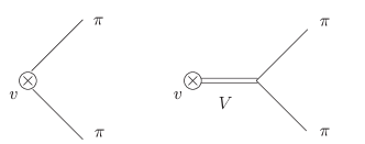
Figure 1: Tree-level contributions to the vector form factor of the pion. A single line stands for a pseudo-Goldstone boson while a double line indicates a resonance.

Within Resonance Chiral Theory the diagrams contributing to the VFF at leading order in $1/N_{C}$ are shown in figure 1. They generate the result

$$\mathcal{F}_{R\chi T}\left(s\right) = 1+\frac{F_{V}G_{V}}{F^{2}}\frac{s}{M_{V}^{2}-s}\,.$$ (6)

Considering that the form factor is constrained to be zero at infinite momentum transfer [26], the vector couplings should satisfy

$$F_{V}G_{V} = F^{2}\,,$$ (7)

which implies

$$\mathcal{F}_{R\chi T}\left(s\right) = \frac{M_{V}^{2}}{M_{V}^{2}-s}\,.$$ (8)

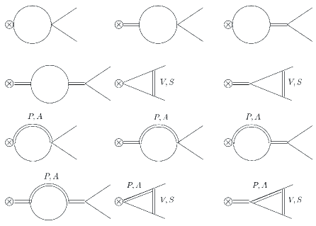
Figure 2: One-loop contributions to the vector form factor of the pion with absorptive cut. A single line stands for a pseudo-Goldstone boson while a double line indicates a resonance.

The subleading corrections can be calculated by means of dispersive relations. Once the one-loop absorptive parts of $\mathcal{F}_{R\chi T}\left(s\right)$ are known, one can reconstruct the full form factor up to appropriate subtraction terms. We can separate then the leading and subleading parts of the amplitude in the form

$$\mathcal{F}_{R\chi T}\left(s\right) = \,\frac{\displaystyle M_{V}^{2}}{\displaystyle M_{V}^{2}-s}\,\,+\,\,\mathcal{F}(s)_{{}_{\rm NLO}}\,,$$ (9)

with $\mathcal{F}(s)^{{}^{\rm NLO}}$ containing the one-loop contribution and the subleading part $\delta_{{}_{\rm NLO}}$ of the resonance coupling combination $F_{V}G_{V}/F^{2}=1+\delta_{{}_{\rm NLO}}$ (for details see appendix E):

$$\mathcal{F}(s)_{{}_{\rm NLO}}\,\,=\,\,\delta_{{}_{\rm NLO}}\,\frac{\displaystyle s}{\displaystyle M_{V}^{2}-s}\,\,+\,\,\mathcal{F}^{1\ell}(s)\,.$$ (10)

The explicit form for the subtracted one-loop amplitude $\mathcal{F}^{1\ell}(s)$ can be found in Appendices A and C, being fully determined by the spectral function Im$\mathcal{F}(s)$ through a once-subtracted dispersion relation. It vanishes at $s=0$ and has no contribution to the real part of the pole at $s=M_{V}^{2}$. The subleading correction to the couplings, $\delta_{{}_{\rm NLO}}$, is fixed by means of the high-energy matching after demanding that it cancels the bad behaviour of $\mathcal{F}^{1\ell}(s)=\delta_{{}_{\rm NLO}}+{\cal O}(s^{-1})$ when $s\to\infty$. Furthermore, the NLO term $\mathcal{F}(s)_{{}_{\rm NLO}}$ can be neatly separated into its different contributions from the various two-meson absorptive channels $\mathcal{F}(s)_{{}_{\rm NLO}}|_{m_{1},m_{2}}$, given by the corresponding $\mathcal{F}^{1\ell}(s)|_{m_{1},m_{2}}$ and the consequent $\delta_{{}_{\rm NLO}}|_{m_{1},m_{2}}$. These details are relegated to Appendices B and C.

Although in this article we follow the procedure of refs. [17, 18], our results can be also derived in an utterly equivalent way through a Feynman diagram computation and the standard renormalization procedure. This derivation is slightly more complex and its detailed explaination is relegated to appendix E.

We will consider only the effects of absorptive loops with two pseudo-Goldstones ($\pi\pi$) or with one pseudo-Goldstone and a resonance ($R\pi$). Two-resonance channels $RR^{\prime}$ have their thresholds at $(M_{R}+M_{R}^{\prime})^{2}\stackrel{{\scriptstyle>}}{{{}_{\sim}}}2$ GeV² and their impact on the LEC determination is expected to be negligible [18]. Taking this into account, we extract our R$\chi$T form factor through the following short-distance matching procedure:

1. Determine the spectral function of the considered absorptive cuts ($\pi\pi$ and $R\pi$). The full expressions are shown in eqs. (32), (33) and (34) of appendix B.

2. We demand Im$\mathcal{F}(s)$ to be well-behaved at high energies, i.e., it must vanish when $s\to\infty$. In the present work, we will actually impose this constraint channel by channel, i.e., we will demand that each separate two-meson cut Im$\mathcal{F}(s)|_{m_{1},m_{2}}$ vanishes at $s\to\infty$. For spin–0 mesons this must be so as its one-loop contribution to the spectral function is essentially its VFF at LO (which vanishes at infinite momentum) times the partial-wave scattering amplitude at LO (which is upper bounded). For higher spin resonances the derivation is more cumbersome as the Lorentz structure allows for the proliferation of form factors and the unitarity relations are not that simple. Still, in many situations it has been already found that amplitudes with massive spin–1 mesons as final states must go to zero at high energies even faster, due to the presence of extra powers of momenta in the unitarity relations coming from intermediate longitudinal polarizations [18]. In summary, we will assume Im$\mathcal{F}(s)|_{m_{1},m_{2}}\to 0$ when $s\to\infty$ for every absorptive two-meson cut under consideration, regardless of the spin of the intermediate mesons.

   In the case of the $\pi\pi$ cut we have found two constraints, which are consistent with the literature,

   $$F_{V}G_{V}\,=\,F^{2}\,,\qquad\qquad 3\,G_{V}^{2}+2\,c_{d}^{2}\,=\,F^{2}\,,$$ (11)

   where the first one coincides with eq. (7), that is, with the constraint obtained with the vector form factor at leading-order [8]. The second one was derived in ref. [27] from the LO $\pi\pi$ scattering amplitude. It is interesting to remark that the $c_{d}=0$ limit of this second relation, $G_{V}=F/\sqrt{3}$, has been obtained recently from a study of $\tau^{-}\to P^{-}\,\gamma\,\nu_{\tau}$ decays ($P=\pi,K$) [28]. We have used these constraints to fix $F_{V}$ and $c_{d}^{2}$.

   For the $P\pi$ cut, the only possible solution is to kill the whole contribution by means of

   $$\lambda_{1}^{\mathrm{PV}}\,=\,0\,,$$ (12)

   which is consistent with the large-$N_{C}$ constraint from the vector form factor into $P\pi$, studied in ref. [18].

   The analysis of the $A\pi$ cut leads to more than one real solution. We have chosen the solutions consistent with previous works [15, 18], where the NLO contributions in $1/N_{C}$ to the $\Pi_{VV}(s)$ correlator coming from tree-level form factors to resonance fields were studied:

   $$-2\lambda_{2}^{\mathrm{VA}}+\lambda_{3}^{\mathrm{VA}}=0\,,\phantom{\frac{1}{2}}\qquad-\lambda_{3}^{\mathrm{VA}}+\lambda_{4}^{\mathrm{VA}}+2\lambda_{5}^{\mathrm{VA}}=\frac{F_{A}}{F_{V}}\,,$$

   $$\lambda_{1}^{\mathrm{SA}}=-\frac{F_{A}\,G_{V}\left(M_{A}^{2}-4\,M_{V}^{2}\right)}{3\sqrt{2}M_{A}^{2}c_{d}\,F_{V}}\,.$$ (13)

   The first two constraints, in the first line, come from the analysis of the $A\pi$ vector form-factor. The last relation with $\lambda_{1}^{SA}$ is then needed to make Im$\mathcal{F}(s)|_{A\pi}\to 0$ for $s\to\infty$.

   After imposing the relations (11), (12) and (13) the spectral functions can be expressed in terms of $G_{V}$, $F_{A}$, $F$ and masses, as shown in eqs. (36), (37) and (38).

3. The spectral function is now ready for the once-subtracted dispersion relation provided in the appendix A in eq. (29), which allows to reconstruct the full form factor up to the pole position at $s=M_{V}^{2}$ and the real part of its residue.

4. Finally, we impose that the whole $\mathcal{F}_{R\chi T}(s)$ vanishes at short distances –not only its imaginary part–. This fixes the real part of the residue at $s=M_{V}^{2}$ and, consequently, the NLO correction $\delta_{\mathrm{NLO}}$ in eq. (10). In order to ease the reading of the manuscript, the complicated expressions for the well-behaved contributions to the different channels are provided in appendix C, in eqs. (39), (40) and (41).

4 The chiral couplings $L_{9}(\mu)$ and $C_{88}(\mu)-C_{90}(\mu)$

The low-momentum expansion of $\mathcal{F}(s)$ is determined by $\chi$PT [2, 23]. The corresponding expression in the chiral limit reads

$$\begin{array}[]{rl}&\mathcal{F}_{\chi PT}\left(s\right)=1+\displaystyle\frac{2\,s}{F^{2}}\left\{L_{9}(\mu)+\frac{\Gamma_{9}}{32\pi^{2}}\left(\frac{5}{3}-\log\frac{-s}{\mu^{2}}\right)\right\}\\ &\qquad-\,\displaystyle\frac{4\,s^{2}}{F^{4}}\left\{C_{88}(\mu)-C_{90}(\mu)-\frac{\Gamma_{88}^{(L)}-\Gamma_{90}^{(L)}}{32\pi^{2}}\left(\frac{5}{3}-\log\frac{-s}{\mu^{2}}\right)+\mathcal{O}\!\left(N_{C}^{0}\right)\right\}+\mathcal{O}\!\left(s^{3}\right)\,,\end{array}$$

with [2, 3]

$$\Gamma_{9}\,=\,\frac{1}{4},\qquad\qquad\Gamma_{88}^{(L)}-\Gamma_{90}^{(L)}\,=\,-\frac{2L_{1}}{3}+\frac{L_{2}}{3}-\frac{L_{3}}{2}+\frac{L_{9}}{4}\,.$$ (14)

The couplings $F^{2}$, $L_{9},\,C_{88}/F^{2}$ and $C_{90}/F^{2}$ are of ${\cal O}(N_{C})$, while $\Gamma_{9}$, $\Gamma_{88}^{(L)}/F^{2}$ and $\Gamma_{90}^{(L)}/F^{2}$ are of ${\cal O}(N_{C}^{0})$ and represent a NLO effect.

The low-energy expansion of eqs. (8) and (9), obtained, respectively, within Resonance Chiral Theory at leading-order and at next-to-leading order in the $1/N_{C}$ expansion, allows to determine the chiral couplings $L_{9}$ and $C_{88}-C_{90}$ at LO and at NLO.

4.1 The large-$N_{C}$ limit

At leading-order in $1/N_{C}$, eq. (4) becomes

$$\mathcal{F}_{\chi PT}\left(s\right)\,=\,1+\frac{2\,s}{F^{2}}\left\{L_{9}+\mathcal{O}\!\left(N_{C}^{0}\right)\right\}-\frac{4\,s^{2}}{F^{4}}\left\{C_{88}-C_{90}+\mathcal{O}\!\left(N_{C}\right)\right\}+\mathcal{O}\!\left(s^{3}\right)\,.$$ (15)

Within R$\chi$T in the large-$N_{C}$ limit, eq. (8) can be now expanded at low energies:

$$\mathcal{F}_{R\chi T}\left(s\right)\,=\,\frac{M_{V}^{2}}{M_{V}^{2}-s}\,=\,1+\frac{s}{M_{V}^{2}}+\frac{s^{2}}{M_{V}^{4}}+\mathcal{O}\!\left(s^{3}\right)\,.$$ (16)

The matching between (15) and (16) fixes $L_{9}$ and $C_{88}-C_{90}$ at LO [8, 9],

$$L_{9}\,=\,\frac{F^{2}}{2M_{V}^{2}}\,,\qquad\qquad C_{88}-C_{90}\,=\,-\frac{F^{4}}{4M_{V}^{4}}\,.$$ (17)

4.2 $L_{9}(\mu)$ and $C_{88}(\mu)-C_{90}(\mu)$ at NLO

Following the same steps as before, let us determine the related $\mathcal{O}(p^{4})$ and $\mathcal{O}(p^{6})$ low-energy constants by matching eq. (4) and the low-energy expansion of eq. (9),

$$\mathcal{F}_{R\chi T}\left(s\right) = 1+\displaystyle\frac{2s}{F^{2}}\left\{\frac{F^{2}}{2M_{V}^{2}}+\bar{\xi}^{(2)}+\frac{\Gamma_{9}}{32\pi^{2}}\left(\frac{5}{3}-\log\frac{-s}{M_{V}^{2}}\right)\right\}$$

$$-\displaystyle\frac{4\,s^{2}}{F^{4}}\left\{-\frac{F^{4}}{4M_{V}^{4}}+\bar{\xi}^{(4)}-\frac{\Gamma_{88}^{(L)}-\Gamma_{90}^{(L)}}{32\pi^{2}}\left(\frac{5}{3}-\log\frac{-s}{M_{V}^{2}}\right)\right\}+\mathcal{O}\!\left(s^{3}\right)\,,$$

where the $\bar{\xi}^{(2n)}$ are the relevant $\mathcal{O}(s^{n})$ coefficients of the low-energy expansion of $\mathcal{F}_{{}_{\rm NLO}}(s)$, once the structure coming from the $\chi$PT one-loop diagram has been subtracted from the $\pi\pi$ channel. The separated contributions $\bar{\xi}^{(2n)}_{m_{1},m_{2}}$ from each absorptive two-meson cut $\mathcal{F}_{{}_{NLO}}(s)|_{m_{1},m_{2}}$ are provided in appendix D, being each of them independent of the renormalization scale $\mu$.

By comparing the $\chi$PT expression (4) to the R$\chi$T low-energy expansion (4.2), it is straightforward to estimate the chiral LECs $L_{9}(\mu)$ and $C_{88}(\mu)-C_{90}(\mu)$ up to NLO in $1/N_{C}$:

$$\begin{array}[]{rl}\qquad\qquad\qquad L_{9}(\mu)\,\,=&\,\,\displaystyle\frac{F^{2}}{2M_{V}^{2}}\,\,+\,\,\bar{\xi}^{(2)}\,\,+\,\,\frac{\Gamma_{9}}{32\pi^{2}}\,\ln\frac{M_{V}^{2}}{\mu^{2}}\,,\\ C_{88}(\mu)\!-\!C_{90}(\mu)\,\,=&\,\,-\displaystyle\frac{F^{4}}{4M_{V}^{2}}\,\,+\,\,\bar{\xi}^{(4)}\,\,-\,\,\frac{\Gamma_{88}^{(L)}-\Gamma_{90}^{(L)}}{32\pi^{2}}\!\,\ln\frac{\displaystyle M_{V}^{2}}{\displaystyle\mu^{2}}\,,\end{array}$$ (19)

where

$$\Gamma_{88}^{(L)}-\Gamma_{90}^{(L)}\;\;=\;\;\frac{3G_{V}^{2}}{8M_{V}^{2}}-\frac{c_{d}^{2}}{4M_{S}^{2}}+\frac{F_{V}G_{V}}{8M_{V}^{2}}\;\;=\;\;\frac{F^{2}-3G_{V}^{2}}{8M_{S}^{2}}-\frac{F^{2}+3G_{V}^{2}}{8M_{V}^{2}}$$ (20)

matches the corresponding ${\cal O}(p^{6})$ running at NLO in $1/N_{C}$. Note that the large–$N_{C}$ relations $L_{2}=2L_{1}=\frac{G_{V}^{2}}{4M_{V}^{2}}$, $L_{3}=-\frac{3G_{V}^{2}}{4M_{V}^{2}}+\frac{c_{d}^{2}}{2M_{S}^{2}}$ and $L_{9}=\frac{F_{V}G_{V}}{2M_{V}^{2}}$ [7] have been used in eq.(14). The high-energy constraints $F_{V}G_{V}=F^{2}$ and $2c_{d}^{2}=F^{2}-3G_{V}^{2}$ of eq. (11) have been employed to obtain the result on the r.h.s. of eq. (20).

4.3 Phenomenology

Using $M_{V}\simeq 0.77\,$GeV and $F\simeq 89\,$MeV, one gets the large-$N_{C}$ estimates from eq. (17): $L_{9}\simeq 6.7\cdot 10^{-3}$ and $C_{88}-C_{90}\simeq-4.5\cdot 10^{-5}$. At $\mu_{0}=770$ MeV, the phenomenological determinations $L_{9}(\mu_{0})=\left(6.9\pm 0.7\right)\cdot 10^{-3}$ [2, 6] and $L_{9}(\mu_{0})=\left(5.93\pm 0.43\right)\cdot 10^{-3},C_{88}(\mu_{0})-C_{90}(\mu_{0})=\left(-5.5\pm 0.5\right)\cdot 10^{-5}$ [23], obtained respectively from an $\mathcal{O}(p^{4})$ and an $\mathcal{O}(p^{6})$ ChPT fit, agree approximately with the LO estimates.

Large–$N_{C}$ estimates are naively expected to approximate well the couplings at scales of the order of the relevant dynamics involved ($\mu\sim M_{R}$). However, they always carry an implicit error because of the uncertainty on $\mu$. This theoretical uncertainty is rather important in couplings generated through scalar meson exchange, such as $L_{8}(\mu)$. In the present case, it also has a moderate importance. The size of the NLO corrections in $1/N_{C}$ to $L_{9}(\mu)$ and $C_{88}(\mu)-C_{90}(\mu)$ can be estimated by regarding their variations with $\mu$. These are respectively given by

$$\frac{\partial\,L_{9}(\mu)}{\partial\log\mu^{2}}\,=\,-\,\frac{\Gamma_{9}}{32\pi^{2}}=-0.8\cdot 10^{-3}\,,\quad\frac{\partial\,\left(C_{88}(\mu)-C_{90}(\mu)\right)}{\partial\log\mu^{2}}=\frac{\Gamma_{88}^{(L)}-\Gamma_{90}^{(L)}}{32\pi^{2}}\simeq 0.9\cdot 10^{-5}\,.$$ (21)

So far, we have been working within a $U(3)_{L}\otimes U(3)_{R}$ framework, but we are actually interested on the couplings of the standard $SU(3)_{L}\otimes SU(3)_{R}$ chiral theory. Thus, a matching between the two versions of $\chi$PT must be performed. Nonetheless, on the contrary to what happens with other matrix elements (e.g. the $S-P$ correlator [17]), the spin–1 two-point functions do not gain contributions from the $U(3)$–singlet chiral pseudo-Goldstone; the $\eta_{1}$ does neither enter at tree-level nor in the one-loop correlators. Therefore, the corresponding LECs are identical in both theories at leading and next-to-leading order in $1/N_{C}$: $L_{9}(\mu)^{U(3)}=L_{9}(\mu)^{SU(3)}$, $\left(C_{88}(\mu)-C_{90}(\mu)\right)^{U(3)}=\left(C_{88}(\mu)-C_{90}(\mu)\right)^{SU(3)}$.

The needed input parameters are defined in the chiral limit. We take the ranges [2, 29] $M_{V}=\left(770\pm 5\right)\,$MeV, $M_{S}=\left(1090\pm 110\right)\,$MeV and $F=\left(89\pm 2\right)\,$MeV. The resonance couplings $G_{V}$ and $F_{A}$ can be fixed in terms of $F$ and masses if one considers the short-distance conditions obeyed by the left–right correlator [6]. The constraint of eq. (7), coming from the vector form factor of the pion, and those from the first and second Weinberg sum rules [22] determine the vector and axial-vector couplings at LO in $1/N_{C}$ [15, 18],

$$F_{V}^{2}=F^{2}\frac{M_{A}^{2}}{M_{A}^{2}-M_{V}^{2}},\qquad G_{V}^{2}=F^{2}\frac{M_{A}^{2}-M_{V}^{2}}{M_{A}^{2}},\qquad F_{A}^{2}=F^{2}\frac{M_{V}^{2}}{M_{A}^{2}-M_{V}^{2}},$$ (22)

with $M_{A}>M_{V}$. Due to the large width of the $a_{1}(1260)$ meson, the determination of the Lagrangian parameter $M_{A}$ is far from trivial. From the observed rates $\Gamma(\rho^{0}\to e^{+}e^{-})=(7.02\pm 0.13)$ keV [29] and $\Gamma\left(a_{1}\to\pi\gamma\right)=(650\pm 250)\,$keV [29], and considering (22), one finds $M_{A}=(938\pm 13)$ MeV and $M_{A}=(960\pm 80)$ MeV. Another large–$N_{C}$ determination of $M_{A}$ was obtained in ref. [30] from the study of the $\pi\to e\nu_{e}\gamma$ decay, which yields $M_{A}=(998\pm 49)$ MeV. We cannot use the information coming from $\Gamma(\rho\to 2\pi)=(149.4\pm 1.0)$ MeV [29] in order to determine $M_{A}$, since $G_{V}$ is constrained by eq. (11) to be smaller than $F/\sqrt{3}$, which results in $M_{A}<940\,$MeV. In spite of the dispersion of values for $M_{A}$, one gets a consistent description in the range $M_{A}=(920\pm 20)\,$MeV, which we will take as our input. The resulting numerical predictions for the LECs are

$$L_{9}(\mu_{0}) = \left(7.9\pm 0.4\right)\cdot 10^{-3}\,,$$

$$C_{88}(\mu_{0})-C_{90}(\mu_{0}) = \left(-4.6\pm 0.4\right)\cdot 10^{-5}\,,$$ (23)

being $\mu_{0}$ the usual renormalization scale, $\mu_{0}=770\,$MeV.

	1st Approach		2nd Approach
$10^{3}\cdot L_{9}$ at LO	$6$.	$68$	$6$.	$68$
$10^{3}\cdot\bar{\xi}^{(2)}_{\pi\pi}$	$0$.	$11$	$-0$.	$04$
$10^{3}\cdot\bar{\xi}^{(2)}_{P\pi}$	$0$.	$00$	$0$.	$00$
$10^{3}\cdot\bar{\xi}^{(2)}_{A\pi}$	$1$.	$12$	$1$.	$00$
$10^{5}\cdot\left(C_{88}-C_{90}\right)$ at LO	$-4$.	$46$	$-4$.	$46$
$10^{5}\cdot\bar{\xi}^{(4)}_{\pi\pi}$	$0$.	$76$	$0$.	$71$
$10^{5}\cdot\bar{\xi}^{(4)}_{P\pi}$	$0$.	$00$	$0$.	$00$
$10^{5}\cdot\bar{\xi}^{(4)}_{A\pi}$	$-0$.	$88$	$-0$.	$73$

Table 1: Different contributions to the chiral couplings within the two numerical approaches explained in the text.

Alternatively, one could also use the phenomenological values for $G_{V}$, $F_{A}$ and the axial-vector mass, instead of fixing them through the Weinberg sum-rules. Thus, one may employ $M_{A}=\left(1200\pm 200\right)\,$MeV [29], and $F_{A}=(120\pm 20)\,$MeV, from the observed rate $\Gamma\left(a_{1}\to\pi\gamma\right)=(650\pm 250)\,$keV [29]. The constraint of eq. (11) implies that $G_{V}<F/\sqrt{3}$, so that we take the range $G_{V}\in[40,50]\,$MeV. For the remaining inputs $M_{V}$, $M_{S}$ and $F$, we consider the same values used before, yielding the predictions

$$L_{9}(\mu_{0}) = \left(7.6\pm 0.6\right)\cdot 10^{-3}\,,$$

$$C_{88}(\mu_{0})-C_{90}(\mu_{0}) = \left(-4.5\pm 0.5\right)\cdot 10^{-5}\,.$$ (24)

As it can be observed, the influence of using the first or the second approach is not crucial at the present level of accuracy. We take the values in (23), which include more theoretical constraints, as our final next-to-leading-order estimates for the LECs.

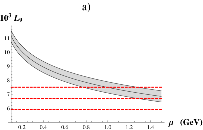
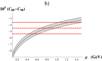
Figure 3: The R$\chi$T predictions (solid gray band) for the $\chi$PT ${\cal O}(p^{4})$ low-energy constant $L_{9}(\mu)$ (a) and the ${\cal O}(p^{6})$ combination $C_{88}(\mu)-C_{90}(\mu)$ (b) are compared to their large–$N_{C}$ estimates (red dashed) for different values of the renormalization scale $\mu$. The error of the large–$N_{C}$ estimate is given by the naive saturation scale uncertainty from eq. (21).

In table 1 we present the different contributions to the LECs within the first and second approaches. A graphical comparison of the NLO predictions and the large–$N_{C}$ estimates has been made in figure 3 for different values of the renormalization scale $\mu$.

It is appropriate to note the appreciable increase of $L_{9}(\mu_{0})$ from the large-$N_{C}$ prediction, for $\mu_{0}=770\,$MeV. In fact, the correction $\delta_{NLO}$ in eq. (10) gets a contribution from the $A\pi$ channel which is still comparable to that from the $\pi\pi$ one. This subleading contribution to $F_{V}G_{V}$, fixed through short-distance matching, increases the value of $L_{9}$ by $1\cdot 10^{-3}$, a quite sizeable shift. For details see appendix E and ref. [31].

5 Conclusions

In this article we have completed the analysis of the VFF at NLO in $1/N_{C}$, initiated in ref. [11], where the general framework was established. We have considered operators with more than one resonance and have studied contributions from intermediate channels with resonances. We get a well-behaved VFF at high-energies, which goes to zero for $q^{2}\to\infty$ [26].

Imposing that each individual absorptive cut vanishes at short distances, one gets stringent constraints on the structure of the VFF, which led to a prediction of the relevant ${\cal O}(p^{4})$ and ${\cal O}(p^{6})$ $\chi$PT  couplings up to NLO in $1/N_{C}$. The required inputs are the resonance masses $M_{V}$, $M_{A}$ and $M_{S}$, and the pion decay constant $F$. As expected for such a well-known observable, the large–$N_{C}$ prediction provides already an excellent estimate and the subleading corrections are relatively small. At the reference scale $\mu_{0}=770$ MeV, we obtain

$$L_{9}(\mu_{0}) = \left(7.9\pm 0.4\right)\cdot 10^{-3}\,,$$

$$C_{88}(\mu_{0})-C_{90}(\mu_{0}) = \left(-4.6\pm 0.4\right)\cdot 10^{-5}\,.$$ (25)

As the matching of R$\chi$T with $\chi$PT is complete up to NLO in $1/N_{C}$, we fully control the running of the LECs up to that order and, e.g., we are able to predict $L_{9}(\mu)$ for any desired value of $\mu$.

	$10^{3}\cdot L_{9}(\mu_{0})$	$10^{5}\cdot\left(C_{88}(\mu_{0})-C_{90}(\mu_{0})\right)$
This work 1st	$7.9\pm 0.4$	$-4.6\pm 0.4$
This work 2nd	$7.6\pm 0.6$	$-4.5\pm 0.5$
Ref. [2]	$6.9\pm 0.7$
Ref. [23]	$5.93\pm 0.43$	$-5.5\pm 0.5$
Ref. [25]	$7.04\pm 0.23$
Ref. [32] at ${\cal O}(p^{4})$	$6.54\pm 0.15$
Ref. [32] at ${\cal O}(p^{6})$	$5.50\pm 0.40$
Ref. [33]	$6.3\pm 0.4$

Table 2: Comparison of our result with other determinations, being $\mu_{0}=770\,$MeV.

This result is in reasonable agreement with previous calculations [2, 23, 25, 32, 33], see table 2, and shows once more the efficacy of R$\chi$T to describe low-energy QCD matrix elements, specially if they are dominated by resonances. It is important to remark not only that the amplitude is dominated by tree-level exchanges but also the fact that the one-loop corrections are not large.

Our determination of $L_{9}(\mu_{0})$ has a larger central value than the result obtained from an ${\cal O}(p^{6})$ chiral fit to the VFF [23] at low energies, and it is closer to the chiral fit determination at ${\cal O}(p^{4})$ [2]. On the other hand, the ALEPH $\tau$-data analysis performed in [25], which is also of ${\cal O}(p^{6})$ but takes higher-energy data into account, yields a value of the order of $7\cdot 10^{-3}$, much closer to our estimate.

In future works, we plan to study the pion scalar form-factor and the LECs $L_{4}(\mu)$ and $L_{5}(\mu)$, where the situation is much less clear since, in that case, one has contributions from broad resonance states like the $f_{0}(600)$.

Appendix A Dispersion relations and loop contribution

One may use a once–subtracted dispersion relation, derived from the identity

$$\frac{\displaystyle\mathcal{F}(s)}{\displaystyle s} = \frac{\displaystyle 1}{\displaystyle 2\pi i}\,\oint\,\ \mathrm{d}t\;\frac{\displaystyle\mathcal{F}(t)}{\displaystyle t\,(t-s)}\,,$$ (26)

where the integration is performed in the usual complex circuit [18]. The form-factor in the integrand can be written as

$$\frac{\displaystyle\mathcal{F}(t)}{\displaystyle t} = \frac{\displaystyle D(t)}{\displaystyle\left(M_{V}^{2}-t\right)^{2}}\,,$$ (27)

where $D(t)$ is an analytical function except for the unitarity logarithmic branch cut and the single pole of $\frac{\mathcal{F}(t)}{t}$ at $t=0$. One gets then

$$\frac{\displaystyle 1}{\displaystyle s}\,\,\mathcal{F}(s) = \frac{\displaystyle 1}{\displaystyle s}\,+\,\frac{\displaystyle 1}{\displaystyle s}\,\mathcal{F}^{1\ell}(s)-\frac{\displaystyle\mbox{Re}D^{\prime}(M_{V}^{2})}{\displaystyle M_{V}^{2}-s}+\frac{\displaystyle\mbox{Re}D(M_{V}^{2})}{\displaystyle\left(M_{V}^{2}-s\right)^{2}}\,,$$ (28)

where the $\frac{1}{s}$ term on the r.h.s. is given by the integration $\frac{1}{2\pi i}\int_{\theta=2\pi^{-}}^{\theta=0^{+}}\frac{dt}{t}\,\frac{\mathcal{F}(t)}{(t-s)}$, with ${t=\epsilon\,e^{i\theta}}$, around $t=0$ of the function $\frac{\mathcal{F}(t)}{t}\approx\frac{1}{t}+{\cal O}(t^{0})$, and the different contributions of each two-meson absorptive cut are given by the dispersive integral,

$$\mathcal{F}^{1\ell}(s)|_{m_{1},m_{2}} = \lim_{\epsilon\to 0}\left[\frac{\displaystyle s}{\displaystyle\pi}\int_{0}^{M_{V}^{2}-\epsilon}\!\!\!\mathrm{d}t\;\frac{\displaystyle\mbox{Im}\mathcal{F}(t)|_{m_{1},m_{2}}}{\displaystyle t\,(t\,-\,s)}\,+\,\frac{\displaystyle s}{\displaystyle\pi}\int_{M_{V}^{2}+\epsilon}^{\infty}\!\!\!\mathrm{d}t\;\frac{\displaystyle\mbox{Im}\mathcal{F}(t)|_{m_{1},m_{2}}}{\displaystyle t\,(t\,-\,s)}\right.$$ (29)

$$\qquad\left.\,-\,\frac{\displaystyle 2s}{\displaystyle\pi\epsilon}\,\lim_{t\to M_{V}^{2}}\left\{(M_{V}^{2}-t)^{2}\,\frac{\displaystyle\mbox{Im}\mathcal{F}(t)|_{m_{1},m_{2}}}{\displaystyle t\,(t\,-\,s)}\right\}\,\,\right]\,.$$

Notice that if the threshold of the channel is above the resonance mass $M_{V}$, then this expression gets simplified into the form

$$\mathcal{F}^{1\ell}(s)|_{m_{1},m_{2}} = \lim_{\epsilon\to 0}\frac{\displaystyle s}{\displaystyle\pi}\int_{(M_{1}+M_{2})^{2}}^{\infty}\!\!\!\mathrm{d}t\;\frac{\displaystyle\mbox{Im}\mathcal{F}(t)|_{m_{1},m_{2}}}{\displaystyle t\,(t\,-\,s)}\,,$$ (30)

with $M_{1}$ ($M_{2}$) the mass of the $m_{1}$ ($m_{2}$) meson.

If we choose the on-shell mass scheme, without double poles in the perturbative expansion, we have then

$$\mathcal{F}(t) = 1\,+\,\sum_{m_{1},m_{2}}\mathcal{F}^{1\ell}(t)|_{m_{1},m_{2}}-\frac{\displaystyle s\,\mbox{Re}D^{\prime}(M_{V}^{2})}{\displaystyle M_{V}^{2}-t}\,,$$ (31)

where $\mbox{Re}D^{\prime}(M_{V}^{2})$ can be identified with $-\frac{F_{V}^{r}G_{V}^{r}}{F^{2}}$ for a convenient renormalization scheme of this combination of vector couplings [17, 18, 19] (see appendix E for further details).

Appendix B The spectral functions $\mathrm{Im}\,\mathcal{F}(s)|_{m_{1},m_{2}}$

In this appendix we show the explicit form of the the spectral functions of the different two-particle absorptive cuts. First we present the functions obtained directly from the Feynman diagrams before imposing any short-distance constraint, i.e., they are badly behaved at high energies.

$$\mathrm{Im}\,\mathcal{F}(s)|_{\pi\pi} =\frac{F^{2}\left(M_{V}^{2}-s\right)+sF_{V}G_{V}}{64\pi F^{6}s^{2}\left(s-M_{V}^{2}\right)}\Bigg{\{}2c_{d}^{2}\left(M_{S}^{4}\log\!\bigg{(}1+\frac{s}{M_{S}^{2}}\bigg{)}\left(-12M_{S}^{2}-6s\right)+s^{3}\right.$$ (32)

$$+12sM_{S}^{4}\!\Bigg{)}\!+\!G_{V}^{2}\!\Bigg{(}\!s^{3}\!-\!6M_{V}^{2}\left(M_{V}^{2}\!+\!2s\right)\left.\!\left(\!\log\!\bigg{(}1\!+\!\frac{s}{M_{V}^{2}}\bigg{)}\left(2M_{V}^{2}\!+\!s\right)\!-\!2s\!\right)\!\right)\!\Bigg{\}}$$

$$+\frac{s^{2}G_{V}\left(F^{2}\left(F_{V}+2G_{V}\right)\left(M_{V}^{2}-s\right)+2sF_{V}G_{V}^{2}\right)}{64\pi F^{6}\left(s-M_{V}^{2}\right)^{2}}+\frac{s}{64\pi F^{2}}\,,$$

$$\mathrm{Im}\,\mathcal{F}(s)|_{P\pi} =\frac{\sqrt{2}c_{d}F_{V}\lambda_{1}^{\mathrm{SP}}\lambda_{1}^{\mathrm{PV}}}{32\pi F^{4}s\left(s-M_{V}^{2}\right)}\Bigg{\{}3M_{P}^{4}\left(4M_{S}^{2}+s\right)-3M_{P}^{2}\left(2M_{S}^{2}+s\right)^{2}-M_{P}^{6}$$ (33)

$$-6M_{S}^{2}\!\left(M_{S}^{2}-M_{P}^{2}\right)\!\left(-M_{P}^{2}+2M_{S}^{2}+s\right)\!\log\!\bigg{(}1\!+\!\frac{s-M_{P}^{2}}{M_{S}^{2}}\bigg{)}+12sM_{S}^{4}+s^{3}\Bigg{\}}$$

$$-\frac{F_{V}G_{V}{\lambda_{1}^{\mathrm{PV}}}^{2}}{32\pi F^{4}s\left(s\!-\!M_{V}^{2}\right)}\Bigg{\{}3M_{P}^{2}\!\left(12sM_{V}^{2}\!+\!4M_{V}^{4}\!+\!s^{2}\right)\!+6M_{V}^{2}\!\left(-3M_{P}^{2}\!\left(M_{V}^{2}\!+\!s\right)\right.$$

$$\left.+M_{P}^{4}+5sM_{V}^{2}+2M_{V}^{4}+2s^{2}\right)\log\!\bigg{(}1\!+\!\frac{s-M_{P}^{2}}{M_{V}^{2}}\bigg{)}-3M_{P}^{4}\left(4M_{V}^{2}+s\right)$$

$$+M_{P}^{6}-s\left(24sM_{V}^{2}+12M_{V}^{4}+s^{2}\right)-\frac{2s\left(s-M_{P}^{2}\right)^{3}}{s-M_{V}^{2}}\Bigg{\}}\,,$$

$$\mathrm{Im}\,\mathcal{F}(s)|_{A\pi} =\frac{-G_{V}\left(s\!-\!M_{A}^{2}\right)^{2}}{32F^{4}\pi M_{A}^{2}s\left(s\!-\!M_{V}^{2}\right)^{2}}\Bigg{\{}\!F_{A}\!\left((2\kappa\!+\!\sigma)M_{A}^{4}\!+\!4s(\kappa\!+\!\sigma)M_{A}^{2}\!+\!s^{2}\sigma\right)\!\left(s\!-\!M_{V}^{2}\right)$$

$$-F_{V}\left(s-M_{A}^{2}\right)\left((2\kappa+\sigma)^{2}M_{A}^{4}+2s\left(\kappa^{2}+4\sigma\kappa+2\sigma^{2}\right)M_{A}^{2}+s^{2}\sigma^{2}\right)\Bigg{\}}\phantom{\frac{1}{2}}\!\!\!\!$$

$$-\frac{G_{V}}{32F^{4}\pi M_{A}^{2}s\left(s-M_{V}^{2}\right)}\Bigg{\{}6\log\!\bigg{(}1+\frac{s-M_{A}^{2}}{M_{V}^{2}}\bigg{)}\left(F_{A}\left(s-M_{V}^{2}\right)\left(M_{A}^{2}-M_{V}^{2}\right)\right.$$

$$\left.\left(\kappa M_{A}^{2}\!+\!\sigma\!\left(M_{V}^{2}\!+\!s\right)\!\right)\!+\!F_{V}\!\left(\!\left(M_{A}^{2}\!-\!s\right)\!\left(M_{A}^{2}\!-\!M_{V}^{2}\right)\!\left(M_{V}^{2}\!+\!s\right)\sigma^{2}\!+\!2\kappa M_{A}^{2}\right.\right.\phantom{\frac{1}{2}}\!\!\!\!$$

$$\left.\left.\left(\!M_{A}^{2}\!-\!s\!\right)\!\left(\!M_{A}^{2}\!-\!M_{V}^{2}\!\right)\!\sigma\!+\!\kappa^{2}M_{A}^{2}\!\left(\!3M_{A}^{4}\!-\!5\!\left(\!M_{V}^{2}\!+\!s\!\right)\!M_{A}^{2}\!+\!\left(\!M_{V}^{2}\!+\!2s\!\right)\!\left(\!2M_{V}^{2}\!+\!s\!\right)\!\right)\!\right)\!\right)\!\phantom{\frac{1}{2}}\!\!\!\!$$

$$M_{V}^{2}\!+\!\left(\!M_{A}^{2}\!-\!s\!\right)\!\left(\!F_{A}\!\left(\!s\!-\!M_{V}^{2}\!\right)\!\left((3\kappa\!+\!\sigma)M_{A}^{4}\!+\!\left((3\sigma\!\!-6\kappa)M_{V}^{2}\!+\!s(3\kappa\!+\!4\sigma\!)\right)\!M_{A}^{2}\right.\right.\phantom{\frac{1}{2}}\!\!\!\!$$

$$\left.\left.+\sigma\!\left(s^{2}\!-\!6M_{V}^{4}\!-\!3sM_{V}^{2}\right)\!\right)\!+\!F_{V}\!\left(\!\left(M_{A}^{2}\!-\!s\right)\!\left(M_{A}^{4}\!+\!4sM_{A}^{2}\!-\!6M_{V}^{4}\!+\!s^{2}\right.\right.\right.\phantom{\frac{1}{2}}\!\!\!\!$$

$$\left.\left.\left.+3\left(M_{A}^{2}-s\right)M_{V}^{2}\right)\sigma^{2}+6\kappa M_{A}^{2}\left(M_{A}^{2}-s\right)\left(M_{A}^{2}-2M_{V}^{2}+s\right)\sigma\right.\right.\phantom{\frac{1}{2}}\!\!\!\!$$

$$\left.\left.+\kappa^{2}M_{A}^{2}\left(7M_{A}^{4}-8\left(3M_{V}^{2}+s\right)M_{A}^{2}+12M_{V}^{4}+s^{2}+24sM_{V}^{2}\right)\right)\right)\Bigg{\}}\phantom{\frac{1}{2}}\!\!\!\!$$

$$+\frac{\sqrt{2}c_{d}\lambda_{1}^{\mathrm{SA}}}{32F^{4}\pi s\left(s-M_{V}^{2}\right)}\Bigg{\{}6\log\!\bigg{(}1+\frac{s-M_{A}^{2}}{M_{S}^{2}}\bigg{)}\left(F_{V}\left(2\kappa M_{S}^{4}+(\kappa-\sigma)M_{S}^{2}\right.\right.$$

$$\left.\left.\left(s-M_{A}^{2}\right)+(\kappa+\sigma)M_{A}^{2}\left(s-M_{A}^{2}\right)\right)+F_{A}\left(M_{A}^{2}-M_{S}^{2}\right)\left(M_{V}^{2}-s\right)\right)M_{S}^{2}\phantom{\frac{1}{2}}\!\!\!\!$$

$$+\left(M_{A}^{2}-s\right)\left(F_{V}\left(3\sigma\left(s-M_{A}^{2}\right)\left(M_{A}^{2}-2M_{S}^{2}+s\right)\right.\right.\phantom{\frac{1}{2}}\!\!\!\!$$ (34)

$$\left.\left.+\kappa\left(4sM_{A}^{2}\!-\!5M_{A}^{4}\!+\!12M_{S}^{4}\!+\!s^{2}\right)\!\right)\!+\!3F_{A}\!\left(M_{A}^{2}\!-\!2M_{S}^{2}\!+\!s\right)\!\left(M_{V}^{2}\!-\!s\right)\!\right)\!\!\Bigg{\}}\,,$$

where we have used the combination of couplings $\kappa$ and $\sigma$,

$$\kappa\,=\,-2\lambda_{2}^{\mathrm{VA}}+\lambda_{3}^{\mathrm{VA}}\,,\qquad\qquad\sigma\,=\,2\lambda_{2}^{\mathrm{VA}}-2\lambda_{3}^{\mathrm{VA}}+\lambda_{4}^{\mathrm{VA}}+2\lambda_{5}^{\mathrm{VA}}\,.$$ (35)

After considering the constraints explained in section 3,

$$\begin{array}[]{rlrl}F_{V}G_{V}&=F^{2}\,,\qquad\quad\phantom{\displaystyle\frac{1}{2}}&3\,G_{V}^{2}+2\,c_{d}^{2}&=F^{2}\,,\\ \lambda_{1}^{\mathrm{PV}}&=0\,,\qquad\quad\phantom{\displaystyle\frac{1}{2}}&\kappa&=0\,,\\ \kappa+\sigma&=\displaystyle\frac{F_{A}}{F_{V}}\,,&\lambda_{1}^{\mathrm{SA}}&=-\displaystyle\frac{F_{A}\,G_{V}\left(M_{A}^{2}-4\,M_{V}^{2}\right)}{3\sqrt{2}M_{A}^{2}c_{d}\,F_{V}}\,,\end{array}$$

the imaginary part of each absorptive cut vanishes at short-distances and the following expressions are found,

$$\mathrm{Im}\,\mathcal{F}(s)|_{\pi\pi} =\frac{M_{V}^{2}}{32\pi F^{4}s^{2}\left(s\!-\!M_{V}^{2}\right)^{2}}\Bigg{\{}3M_{S}^{4}\!\left(F^{2}\!-\!3G_{V}^{2}\right)\!\left(M_{V}^{2}\!-\!s\right)\!\log\!\bigg{(}1\!+\!\frac{s}{M_{S}^{2}}\bigg{)}\!\left(2M_{S}^{2}+s\right)$$

$$+G_{V}^{2}M_{V}^{2}\Bigg{(}\log\!\bigg{(}1+\frac{s}{M_{V}^{2}}\bigg{)}\left(-6s^{3}-9s^{2}M_{V}^{2}+6M_{V}^{6}+9sM_{V}^{4}\right)+13s^{3}$$ (36)

$$\Bigg{.}-6s^{2}M_{V}^{2}-6sM_{V}^{4}\Bigg{)}+6sM_{S}^{4}\left(F^{2}-3G_{V}^{2}\right)\left(s-M_{V}^{2}\right)\Bigg{\}}\,,$$

$$\mathrm{Im}\,\mathcal{F}(s)|_{P\pi} =0\,,$$ (37)

$$\mathrm{Im}\,\mathcal{F}(s)|_{A\pi} =\frac{F_{A}^{2}G_{V}^{2}\left(M_{V}^{2}\!-\!M_{A}^{2}\right)}{32\pi F^{6}sM_{A}^{2}\left(s\!-\!M_{V}^{2}\right)^{2}}\Bigg{\{}M_{A}^{4}\Bigg{(}2M_{S}^{2}\left(M_{V}^{2}\!-s\right)\left(\log\!\bigg{(}1\!+\frac{s-M_{A}^{2}}{M_{S}^{2}}\bigg{)}\!-\!1\right)$$

$$+4sM_{V}^{2}-7M_{V}^{4}-3s^{2}\Bigg{)}+2M_{A}^{2}\left(s^{2}M_{V}^{2}\left(3\log\!\bigg{(}1+\frac{s-M_{A}^{2}}{M_{V}^{2}}\bigg{)}-2\right)\right.$$

$$\left.+M_{S}^{4}\left(s-M_{V}^{2}\right)\log\!\bigg{(}1+\frac{s-M_{A}^{2}}{M_{S}^{2}}\bigg{)}-M_{S}^{2}\left(s-M_{V}^{2}\right)\right.$$ (38)

$$\left.\left(s\!-\!4M_{V}^{2}\left(\log\!\bigg{(}1\!+\!\frac{s\!-\!M_{A}^{2}}{M_{S}^{2}}\bigg{)}\!-\!1\right)\right)\!-\!3M_{V}^{6}\left(\log\!\bigg{(}1\!+\!\frac{s\!-\!M_{A}^{2}}{M_{V}^{2}}\bigg{)}\!-1\right)\right)$$

$$+M_{V}^{2}\!\left(s^{2}M_{V}^{2}\!\left(7\!-\!6\log\!\bigg{(}1\!+\!\frac{s\!-\!M_{A}^{2}}{M_{V}^{2}}\bigg{)}\right)\!+\!8M_{S}^{4}\left(M_{V}^{2}\!-\!s\right)\log\!\bigg{(}1\!+\!\frac{s\!-\!M_{A}^{2}}{M_{S}^{2}}\bigg{)}\right.$$

$$\left.+6M_{V}^{6}\log\!\bigg{(}1\!+\!\frac{s\!-\!M_{A}^{2}}{M_{V}^{2}}\bigg{)}\!+\!8sM_{S}^{2}\left(s\!-\!M_{V}^{2}\right)\!-\!6sM_{V}^{4}\!\right)\!+\!2sM_{A}^{6}\!+\!M_{A}^{8}\!\Bigg{\}}.$$

Appendix C Next-to-leading-order corrections $\mathcal{F}_{{}_{\rm NLO}}(s)|_{m_{1},m_{2}}$

In this appendix we show the explicit form of the NLO corrections generated by the considered two-particle absorptive cuts, eqs. (36), (37) and (38), which have been calculated by using the dispersive method discussed in appendix A. Below, we have summed up the $\delta_{{}_{\rm NLO}}$ contribution to $\mathcal{F}^{1\ell}(s)$, as seen in eq. (10), being the different $\mathcal{F}_{{}_{\rm NLO}}(s)|_{m_{1}m_{2}}$ well-behaved at high energies:

$$\mathcal{F}_{{}_{\rm NLO}} \!\!\!\!(s)|_{\pi\pi}=\frac{M_{V}^{2}}{64\pi^{2}F^{4}s\left(s-M_{V}^{2}\right)^{2}}\Bigg{\{}-12M_{S}^{6}\left(F^{2}-3G_{V}^{2}\right)\left(s-M_{V}^{2}\right)f\!\left(s,M_{S}^{2}\right)\Bigg{.}$$ (39)

$$\Bigg{.}-6M_{S}^{4}\left(F^{2}-3G_{V}^{2}\right)\left(s-M_{V}^{2}\right)\left(sf\!\left(s,M_{S}^{2}\right)+2\log\bigg{(}\frac{-s}{M_{S}^{2}}\bigg{)}-2\right)$$

$$\Bigg{.}+G_{V}^{2}M_{V}^{2}\Bigg{(}-6\left(3s^{2}M_{V}^{2}-3sM_{V}^{4}-2M_{V}^{6}+2s^{3}\right)f\!\left(s,M_{V}^{2}\right)$$

$$\Bigg{.}\left.+s^{2}\left(-26\log\bigg{(}\frac{-s}{M_{V}^{2}}\bigg{)}+27\right)+12M_{V}^{4}\left(\log\bigg{(}\frac{-s}{M_{V}^{2}}\bigg{)}-1\right)\right.\Bigg{.}$$

$$\left.\Bigg{.}+3sM_{V}^{2}\left(4\log\bigg{(}\frac{-s}{M_{V}^{2}}\bigg{)}-5\right)\right)+3sM_{S}^{2}\left(F^{2}-3G_{V}^{2}\right)\left(s-M_{V}^{2}\right)\Bigg{\}}\,,$$

$$\mathcal{F}_{{}_{\rm NLO}} \!\!\!\!(s)|_{P\pi}=0\,,$$ (40)

$$\mathcal{F}_{{}_{\rm NLO}} \!\!\!\!(s)|_{A\pi}=-\frac{F_{A}^{2}G_{V}^{2}\left(M_{A}^{2}-M_{V}^{2}\right)}{32\pi^{2}F^{6}sM_{A}^{2}M_{V}^{4}\left(s-M_{V}^{2}\right)^{2}}\Bigg{\{}M_{A}^{4}M_{V}^{4}\Bigg{(}2sM_{S}^{2}\left(M_{V}^{2}-s\right)g\left(s,M_{A}^{2},M_{S}^{2}\right)$$ (41)

$$\Bigg{.}\left.-6s^{2}\log\!\bigg{(}\!1-\frac{M_{V}^{2}}{M_{A}^{2}}\!\bigg{)}\!+\log\!\bigg{(}\!1-\frac{s}{M_{A}^{2}}\!\bigg{)}\!\left(3s^{2}\!+\!2M_{S}^{2}\!\left(M_{V}^{2}-s\right)\!+\!7M_{V}^{4}\!-\!4sM_{V}^{2}\!\right)\!\!\right)\Bigg{.}$$

$$\Bigg{.}+sM_{V}^{6}\left(M_{V}^{2}\left(-6\left(s^{2}-M_{V}^{4}\right)g\left(s,M_{A}^{2},M_{V}^{2}\right)+6M_{V}^{2}\left(\log\bigg{(}1-\frac{s}{M_{A}^{2}}\bigg{)}-1\right.\right.\right.\Bigg{.}$$

$$\Bigg{.}\left.\left.\left.+\log\bigg{(}\frac{M_{A}^{2}}{M_{V}^{2}}\bigg{)}\!\right)\!+s\!\left(\!-7\log\!\bigg{(}1-\frac{s}{M_{A}^{2}}\bigg{)}\!-6\log\!\bigg{(}\frac{M_{A}^{2}}{M_{V}^{2}}\bigg{)}\!+\log\!\bigg{(}1-\frac{M_{V}^{2}}{M_{A}^{2}}\bigg{)}\!+6\!\right)\!\right)\right.\Bigg{.}$$

$$\Bigg{.}\left.+8M_{S}^{4}\!\left(M_{V}^{2}-s\right)\!g\!\left(s,M_{A}^{2},M_{S}^{2}\right)\!-\!8M_{S}^{2}\!\left(s-M_{V}^{2}\right)\!\left(\!\log\!\bigg{(}1\!-\!\frac{s}{M_{A}^{2}}\!\bigg{)}\!+\log\!\bigg{(}\frac{M_{A}^{2}}{M_{S}^{2}}\bigg{)}\!\right.\right.\Bigg{.}$$

$$-1\!\Bigg{)}\!\Bigg{)}\!+M_{A}^{2}M_{V}^{4}\!\left(\!M_{V}^{2}\!\left(\!6\left(s^{3}-sM_{V}^{4}\right)g\left(s,M_{A}^{2},M_{V}^{2}\right)+s^{2}\!\left(\!4\log\bigg{(}1-\frac{s}{M_{A}^{2}}\bigg{)}\right.\right.\right.\Bigg{.}$$

$$\Bigg{.}\left.\left.\left.+2\log\bigg{(}1-\frac{M_{V}^{2}}{M_{A}^{2}}\bigg{)}-7\right)-6M_{V}^{4}\log\bigg{(}1-\frac{s}{M_{A}^{2}}\bigg{)}+7sM_{V}^{2}\right)\right.\Bigg{.}$$

$$\Bigg{.}\left.+2sM_{S}^{4}\left(s-M_{V}^{2}\right)g\left(s,M_{A}^{2},M_{S}^{2}\right)\right.\Bigg{.}$$

$$\Bigg{.}\left.+2M_{S}^{2}\!\left(s-M_{V}^{2}\right)\!\left(\!4sM_{V}^{2}g\left(s,M_{A}^{2},M_{S}^{2}\right)\!+s\!\left(\!\log\!\bigg{(}1-\frac{s}{M_{A}^{2}}\bigg{)}\!+\log\!\bigg{(}\frac{M_{A}^{2}}{M_{S}^{2}}\bigg{)}\!-1\!\right)\right.\right.\Bigg{.}$$

$$\Bigg{.}\left.\left.+4M_{V}^{2}\log\bigg{(}1-\frac{s}{M_{A}^{2}}\bigg{)}\right)\right)+M_{A}^{8}\left(s^{2}\log\bigg{(}1-\frac{M_{V}^{2}}{M_{A}^{2}}\bigg{)}-M_{V}^{4}\log\bigg{(}1-\frac{s}{M_{A}^{2}}\bigg{)}\right)\Bigg{.}$$

$$\Bigg{.}+sM_{A}^{6}M_{V}^{2}\!\left(\!M_{V}^{2}\!\left(\!-2\log\!\bigg{(}1-\frac{s}{M_{A}^{2}}\bigg{)}\!-\!1\!\right)\!+2s\log\!\bigg{(}1-\frac{M_{V}^{2}}{M_{A}^{2}}\bigg{)}\!+s\right)\!\Bigg{\}}\,,$$

where the functions $f(s,M^{2})$ and $g(s,M_{1}^{2},M_{2}^{2})$ have been introduced for simplicity,

$$f\left(s,M^{2}\right) = \frac{1}{s}\left(\mathrm{Li}_{2}\bigg{(}1+\frac{s}{M^{2}}\bigg{)}-\frac{\pi^{2}}{6}\right)\,,$$

$$g\left(s,M_{1}^{2},M_{2}^{2}\right) = \frac{1}{s}\left(\mathrm{Li}_{2}\bigg{(}1+\frac{s}{M_{2}^{2}}-\frac{M_{1}^{2}}{M_{2}^{2}}\bigg{)}-\mathrm{Li}_{2}\bigg{(}1-\frac{M_{1}^{2}}{M_{2}^{2}}\bigg{)}\right)\,.$$ (42)

Appendix D NLO contributions to $L_{9}(\mu)$ and $C_{88}(\mu)-C_{90}(\mu)$

In this appendix we give the full expressions of the NLO contributions to $L_{9}(\mu)$ and $C_{88}(\mu)-C_{90}(\mu)$, following the notation of eqs. (4.2) and (19), i.e., $\bar{\xi}^{(2)}_{m_{1},m_{2}}$ and $\bar{\xi}^{(4)}_{m_{1},m_{2}}$:

$$\bar{\xi}^{(2)}_{\pi\pi} = \frac{1}{768\pi^{2}F^{2}}\Bigg{\{}F^{2}\left(6\log\!\bigg{(}\frac{M_{S}^{2}}{M_{V}^{2}}\bigg{)}-11\right)+G_{V}^{2}\left(38-18\log\!\bigg{(}\frac{M_{S}^{2}}{M_{V}^{2}}\bigg{)}\right)\Bigg{\}}\,,$$ (43)

$$\bar{\xi}^{(2)}_{P\pi} = 0\,,$$ (44)

$$\bar{\xi}^{(2)}_{A\pi} = \frac{F_{A}^{2}G_{V}^{2}}{128\pi^{2}F^{4}M_{A}^{2}M_{V}^{8}\left(M_{A}^{2}-M_{S}^{2}\right)}\Bigg{\{}2M_{A}^{10}\left(M_{S}^{2}-M_{A}^{2}\right)\log\!\bigg{(}1-\frac{M_{V}^{2}}{M_{A}^{2}}\bigg{)}$$ (45)

$$-2M_{A}^{8}M_{V}^{2}\left(M_{A}^{2}-M_{S}^{2}\right)\left(\log\!\bigg{(}1-\frac{M_{V}^{2}}{M_{A}^{2}}\bigg{)}+1\right)+M_{A}^{6}M_{V}^{4}\left(M_{A}^{2}-M_{S}^{2}\right)$$

$$\left(\!16\log\!\bigg{(}1\!-\!\frac{M_{V}^{2}}{M_{A}^{2}}\bigg{)}\!-\!3\right)\!+\!M_{A}^{4}M_{V}^{6}\!\left(\!M_{S}^{2}\!\left(\!-2\log\!\bigg{(}\frac{M_{A}^{2}}{M_{S}^{2}}\bigg{)}\!+\!16\log\!\bigg{(}1\!-\!\frac{M_{V}^{2}}{M_{A}^{2}}\bigg{)}\!-11\right)\right.$$

$$\left.+M_{A}^{2}\left(11\!-\!16\log\!\bigg{(}1\!-\!\frac{M_{V}^{2}}{M_{A}^{2}}\bigg{)}\right)\right)\!+\!M_{A}^{2}M_{V}^{8}\left(M_{S}^{2}\left(10\log\!\bigg{(}\frac{M_{A}^{2}}{M_{S}^{2}}\bigg{)}\!-\!12\log\!\bigg{(}\frac{M_{A}^{2}}{M_{V}^{2}}\bigg{)}\right.\right.$$

$$\left.\left.-2\log\!\bigg{(}1-\frac{M_{V}^{2}}{M_{A}^{2}}\bigg{)}+11\right)+M_{A}^{2}\left(12\log\!\bigg{(}\frac{M_{A}^{2}}{M_{V}^{2}}\bigg{)}+2\log\!\bigg{(}1-\frac{M_{V}^{2}}{M_{A}^{2}}\bigg{)}-11\right)\right)$$

$$+M_{V}^{10}\left(M_{A}^{2}\left(-6\log\!\bigg{(}\frac{M_{A}^{2}}{M_{V}^{2}}\bigg{)}+2\log\!\bigg{(}1-\frac{M_{V}^{2}}{M_{A}^{2}}\bigg{)}+5\right)\right.$$

$$\left. -M_{S}^{2}\left(8\log\!\bigg{(}\frac{M_{A}^{2}}{M_{S}^{2}}\bigg{)}-6\log\!\bigg{(}\frac{M_{A}^{2}}{M_{V}^{2}}\bigg{)}+2\log\!\bigg{(}1-\frac{M_{V}^{2}}{M_{A}^{2}}\bigg{)}+5\right)\right)\Bigg{\}}\,,$$

$$\bar{\xi}^{(4)}_{\pi\pi} = \frac{1}{3072\pi^{2}M_{V}^{2}}\Bigg{\{}2F^{2}\left(11-6\log\!\bigg{(}\frac{M_{S}^{2}}{M_{V}^{2}}\bigg{)}\right)+G_{V}^{2}\left(36\log\!\bigg{(}\frac{M_{S}^{2}}{M_{V}^{2}}\bigg{)}-11\right)\Bigg{\}}$$ (46)

$$+\frac{\left(F^{2}-3G_{V}^{2}\right)}{3072\pi^{2}M_{S}^{2}}\Bigg{\{}12\log\!\bigg{(}\frac{M_{S}^{2}}{M_{V}^{2}}\bigg{)}-19\Bigg{\}}\,,$$

$$\bar{\xi}^{(4)}_{P\pi} = 0\,,$$ (47)

$$\bar{\xi}^{(4)}_{A\pi} = \frac{-F_{A}^{2}G_{V}^{2}}{384\pi^{2}F^{2}M_{A}^{2}M_{V}^{10}\left(M_{A}^{2}-M_{S}^{2}\right)^{2}\left(M_{A}^{2}-M_{V}^{2}\right)}\Bigg{\{}-6M_{A}^{10}M_{V}^{2}\left(M_{A}^{2}-M_{S}^{2}\right)^{2}$$

$$+8M_{V}^{14}\!\left(\!M_{S}^{2}\!\left(\!\log\!\bigg{(}\frac{M_{A}^{2}}{M_{S}^{2}}\bigg{)}\!+\!1\!\right)\!-\!M_{A}^{2}\!\right)\!-\!M_{V}^{12}\!\left(\!2M_{A}^{2}M_{S}^{2}\!\left(\!3\log\!\bigg{(}\frac{M_{A}^{2}}{M_{S}^{2}}\bigg{)}\!+\!6\log\!\bigg{(}\frac{M_{A}^{2}}{M_{V}^{2}}\bigg{)}\right.\right.$$

$$\left.\left.-6\log\!\bigg{(}1\!-\!\frac{M_{V}^{2}}{M_{A}^{2}}\bigg{)}\!+\!4\!\right)\!+\!M_{S}^{4}\!\left(\!12\log\!\bigg{(}\frac{M_{A}^{2}}{M_{S}^{2}}\bigg{)}\!-\!6\log\!\bigg{(}\frac{M_{A}^{2}}{M_{V}^{2}}\bigg{)}\!+\!6\log\!\bigg{(}1\!-\!\frac{M_{V}^{2}}{M_{A}^{2}}\bigg{)}\!+\!5\!\right)\right.$$

$$\left.+M_{A}^{4}\left(-6\log\!\bigg{(}\frac{M_{A}^{2}}{M_{V}^{2}}\bigg{)}+6\log\!\bigg{(}1-\frac{M_{V}^{2}}{M_{A}^{2}}\bigg{)}-13\right)\right)-3M_{A}^{2}M_{V}^{10}\Bigg{(}M_{A}^{2}M_{S}^{2}$$

$$\left.\left(\!5\log\!\bigg{(}\frac{M_{A}^{2}}{M_{S}^{2}}\bigg{)}\!-\!12\log\!\bigg{(}\frac{M_{A}^{2}}{M_{V}^{2}}\bigg{)}\!+\!22\!\right)\!+\!M_{S}^{4}\!\left(\!-9\log\!\bigg{(}\frac{M_{A}^{2}}{M_{S}^{2}}\bigg{)}\!+\!6\log\!\bigg{(}\frac{M_{A}^{2}}{M_{V}^{2}}\bigg{)}\!-\!13\right)\right.$$

$$\left.+M_{A}^{4}\left(6\log\!\bigg{(}\frac{M_{A}^{2}}{M_{V}^{2}}\bigg{)}-9\right)\right)+2M_{A}^{4}M_{V}^{8}\left(M_{A}^{2}M_{S}^{2}\left(8\log\!\bigg{(}\frac{M_{A}^{2}}{M_{S}^{2}}\bigg{)}-18\log\!\bigg{(}\frac{M_{A}^{2}}{M_{V}^{2}}\bigg{)}\right.\right.$$

$$\left.\left.-54\log\!\bigg{(}1\!-\!\frac{M_{V}^{2}}{M_{A}^{2}}\bigg{)}\!+\!71\!\right)\!+\!9M_{S}^{4}\!\left(\!\log\!\bigg{(}\frac{M_{A}^{2}}{M_{V}^{2}}\bigg{)}\!\!-\log\!\bigg{(}\frac{M_{A}^{2}}{M_{S}^{2}}\bigg{)}\!+\!3\log\!\bigg{(}1\!-\!\frac{M_{V}^{2}}{M_{A}^{2}}\bigg{)}\!-\!4\!\right)\right.$$

$$\left.+M_{A}^{4}\left(9\log\!\bigg{(}\frac{M_{A}^{2}}{M_{V}^{2}}\bigg{)}+27\log\!\bigg{(}1-\frac{M_{V}^{2}}{M_{A}^{2}}\bigg{)}-35\right)\right)-M_{A}^{6}M_{V}^{6}\left(M_{A}^{2}-M_{S}^{2}\right)$$

$$\left(\!M_{S}^{2}\!\left(\!3\log\!\bigg{(}\frac{M_{A}^{2}}{M_{S}^{2}}\bigg{)}\!-\!96\log\!\bigg{(}1\!-\!\frac{M_{V}^{2}}{M_{A}^{2}}\bigg{)}\!+\!47\!\right)\!+\!M_{A}^{2}\!\left(\!96\log\!\bigg{(}1\!-\!\frac{M_{V}^{2}}{M_{A}^{2}}\bigg{)}\!-\!47\!\right)\!\right)$$

$$+\!3M_{A}^{8}M_{V}^{4}\!\left(\!M_{A}^{2}\!-\!M_{S}^{2}\!\right)^{2}\!\left(\!18\log\!\bigg{(}1\!-\!\frac{M_{V}^{2}}{M_{A}^{2}}\bigg{)}\!-\!1\!\right)\!-\!6M_{A}^{12}\!\left(\!M_{A}^{2}\!-\!M_{S}^{2}\!\right)^{2}\!\log\!\bigg{(}1\!-\!\frac{M_{V}^{2}}{M_{A}^{2}}\bigg{)}\!\Bigg{\}}\,.$$

Appendix E Description in terms of Feynman diagrams

The subleading corrections can be calculated by means of dispersive relations. Once the NLO absorptive parts of $\mathcal{F}_{R\chi T}\left(s\right)$ are known, one can reconstruct the full form factor up to appropriate subtraction terms. Alternatively, we can compute and separate the tree-level and one-loop amplitudes in the form

$$\mathcal{F}_{R\chi T}\left(s\right) = 1\,+\,\frac{\displaystyle F_{V}G_{V}}{\displaystyle F^{2}}\frac{\displaystyle s}{\displaystyle M_{V}^{2}\,-\,s}\,+\,\frac{\displaystyle 2\widetilde{L}_{9}}{\displaystyle F^{2}}\,s\,\,\,\,+\sum_{m_{1},m_{2}}\mathcal{F}(s)|_{m_{1},m_{2}}\,,$$ (49)

where the one-loop diagrams $\mathcal{F}(s)|_{m_{1},m_{2}}$ can be rewritten by means of a once-subtracted dispersion relation in the form

$$\sum_{m_{1},m_{2}}\mathcal{F}(s)|_{m_{1},m_{2}}=\sum_{m_{1},m_{2}}\mathcal{F}^{1\ell}(s)|_{m_{1},m_{2}}\,+\,\frac{\displaystyle 2\hat{\delta}_{2}}{\displaystyle F^{2}}\,s\,\,\,\,+\,\,\hat{\delta}_{0}\frac{\displaystyle s}{\displaystyle M_{V}^{2}\,-\,s}\,\,+\,\,\hat{\delta}_{-2}\frac{\displaystyle s}{\displaystyle(M_{V}^{2}\,-\,s)^{2}}\,.$$ (50)

The finite part of the loops is contained in the once-subtracted dispersive functions $\mathcal{F}^{1\ell}(s)|_{m_{1},m_{2}}$, fully determined by the imaginary part of Im$\mathcal{F}(s)|_{m_{1},m_{2}}$ through eq. (29). The real parameters $\hat{\delta}_{-2,0,2}$ contain the ultraviolet divergences of the loops, being $\hat{\delta}_{0}$ and $\hat{\delta}_{-2}$ the real part of the pole residues. The local R$\chi$T coupling $\widetilde{L}_{9}$ renormalizes $\hat{\delta}_{2}$, the combination $F_{V}G_{V}$ cancels the divergences in $\hat{\delta}_{0}$ and a convenient shift of the mass, $M_{V}^{(B)\,\,2}=M_{V}^{2}+\delta M_{V}^{2}$ removes the divergent part of $\hat{\delta}_{-2}$. Indeed, we will work in the on-shell scheme and the counterterm $\delta M_{V}^{2}$ will be chosen to completely kill $\hat{\delta}_{-2}$.

In order to finish the short-distance matching we just need to take into account that the once-subtracted loop contribution behaves at short distances like

$$\sum_{m_{1},m_{2}}\mathcal{F}^{1\ell}(s)|_{m_{1},m_{2}}\,\,\,\stackrel{{\scriptstyle s\to\infty}}{{\longrightarrow}}\,\,\,\delta_{0}\,\,\,+\,\,\,{\cal O}(s^{-1})\,,$$ (51)

with $\delta_{0}$ a constant number (denoted before in the text as $\delta_{{}_{NLO}}$). This leads to the VFF high-energy constraints

$$\frac{\displaystyle F_{V}G_{V}}{\displaystyle F^{2}}+\hat{\delta}_{0} = 1+\delta_{0}\,,$$

$$\widetilde{L}_{9}+\hat{\delta}_{2} = 0\,.$$ (52)

Hence, the VFF finally takes the well-behaved structure (9) employed in the article,

$$\mathcal{F}(s)\, = \,1\,\,\,+\,\,\,\big{(}1+\delta_{0}\big{)}\,\frac{\displaystyle s}{\displaystyle M_{V}^{2}-s}\,\,\,+\,\,\,\sum_{m_{1},m_{2}}\mathcal{F}^{1\ell}(s)|_{m_{1},m_{2}}$$ (53)

$$=\,\frac{\displaystyle M_{V}^{2}}{\displaystyle M_{V}^{2}-s}\,+\,\mathcal{F}_{{}_{\rm NLO}}(s)\,.$$

Notice that no real double pole term $\hat{\delta}_{-2}$ remains in our perturbative NLO expression as we have chosen the on-shell mass scheme.

References

• [1] S. Weinberg, Phenomenological Lagrangians, Physica A 96 (1979) 327.
• [2] J. Gasser and H. Leutwyler, Chiral perturbation theory to one loop, Annals Phys. 158 (1984) 142; Chiral perturbation theory: expansions in the mass of the strange quark, Nucl. Phys. B 250 (1985) 465; Low-energy expansion of meson form factors, Nucl. Phys.  B 250 (1985) 517.
• [3] J. Bijnens, G. Colangelo and G. Ecker, The mesonic chiral Lagrangian of order $p^{6}$, JHEP 9902 (1999) 020 [arXiv:hep-ph/9902437]; Renormalization of chiral perturbation theory to order $p^{6}$, Annals Phys.  280 (2000) 100 [arXiv:hep-ph/9907333].
• [4] G. ’t Hooft, A planar diagram theory for strong interactions, Nucl. Phys. B 72 (1974) 461; 75 (1974) 461;
E. Witten, Baryons in the $1/N$ expansion, Nucl. Phys. B 160 (1979) 57.
• [5] M. Knecht and E. de Rafael, Patterns of spontaneous chiral symmetry breaking in the large–$N_{C}$ limit of QCD–like theories, Phys. Lett. B 424 (1998) 335 [arXiv:hep-ph/9712457];
S. Peris, M. Perrottet and E. de Rafael, Matching long and short distances in large–$N_{C}$ QCD, JHEP 9805 (1998) 011 [arXiv:hep-ph/9805442];
M. Golterman and S. Peris, Large–$N_{C}$ QCD meets Regge theory, JHEP 0101 (2001) 028 [arXiv:hep-ph/0101098].
• [6] A. Pich, Low-Energy Constants from Resonance Chiral Theory, [arXiv:0812.2631 [hep-ph]].
• [7] G. Ecker, J. Gasser, A. Pich and E. de Rafael, The role of resonances in chiral perturbation theory, Nucl. Phys. B 321 (1989) 311.
• [8] G. Ecker, J. Gasser, H. Leutwyler, A. Pich and E. de Rafael, Chiral Lagrangians for massive spin 1 fields, Phys. Lett. B 223 (1989) 425.
• [9] V. Cirigliano, G. Ecker, M. Eidemüller, R. Kaiser, A. Pich and J. Portolés, Towards a consistent estimate of the chiral low-energy constants, Nucl. Phys. B 753 (2006) 139 [arXiv:hep-ph/0603205].
• [10] O. Catà and S. Peris, An example of resonance saturation at one loop, Phys. Rev. D 65 (2002) 056014 [arXiv:hep-ph/0107062].
• [11] I. Rosell, J. J. Sanz-Cillero and A. Pich, Quantum loops in the resonance chiral theory: the vector form factor, JHEP 0408 (2004) 042 [arXiv:hep-ph/0407240].
• [12] I. Rosell, P. Ruiz-Femenía and J. Portolés, One-loop renormalization of resonance chiral theory: scalar and pseudoscalar resonances, JHEP 0512 (2005) 020 [arXiv:hep-ph/0510041].
• [13] J.J. Sanz-Cillero, On the structure of two-point Green-functions at next-to-leading order in $1/N_{C}$, Phys. Lett. B 649 (2007) 180-185 [arXiv:hep-ph/0702217];
L.Y. Xiao and J.J. Sanz-Cillero, Renormalizable sectors in resonance chiral theory: $S\to\pi\pi$ decay amplitude, Phys. Lett. B 659 (2008) 452-456 [arXiv:0705.3899 [hep-ph]].
• [14] I. Rosell, P. Ruiz-Femenía and J. Portolés, Vanishing chiral couplings in the large-N(c) resonance theory, Phys. Rev.  D 75 (2007) 114011 [arXiv:hep-ph/0611375];
I. Rosell, P. Ruiz-Femenía and J. J. Sanz-Cillero, Resonance saturation of the chiral couplings at NLO in 1/Nc, Phys. Rev.  D 79 (2009) 076009 [arXiv:0903.2440 [hep-ph]].
• [15] I. Rosell, Quantum corrections in the resonance chiral theory, Ph. D. Thesis (Advisors: Antonio Pich, Jorge Portolés) [arXiv:hep-ph/0701248].
• [16] K. Kampf, J. Novotny and J. Trnka, Renormalization and additional degrees of freedom within the chiral effective theory for spin-1 resonances, Phys. Rev. D 81 (2010) 116004 [arXiv:0912.5289 [hep-ph]].
• [17] I. Rosell, J.J. Sanz-Cillero and A. Pich, Towards a determination of the chiral couplings at NLO in $1/N_{C}$: $L^{r}_{8}(\mu)$ and $C_{38}^{r}(\mu)$, JHEP 0701 (2007) 039. [arXiv:hep-ph/0610290].
• [18] A. Pich, I. Rosell and J. J. Sanz-Cillero, Form-factors and current correlators: chiral couplings $L_{10}(\mu)$ and $C_{87}(\mu)$ at NLO in $1/N_{C}$, JHEP 0807 (2008) 014 [arXiv:0803.1567 [hep-ph]].
• [19] J.J. Sanz-Cillero and J. Trnka, High energy constraints in the octet SS-PP correlator and resonance saturation at NLO in $1/N_{C}$, Phys. Rev. D 81 (2010) 056005 [arXiv:0912.0495 [hep-ph]].
• [20] J. Bijnens, E. Gámiz, E. Lipartia and J. Prades, QCD short-distance constraints and hadronic approximations, JHEP 0304 (2003) 055 [arXiv:hep-ph/0304222];
S. Peris, Large–$N_{C}$ QCD and Pade approximant theory, Phys. Rev. D 74 (2006) 054013 [arXiv:hep-ph/0603190];
P. Masjuan and S. Peris, A Rational approach to resonance saturation in large–$N_{C}$ QCD, JHEP 0705 (2007) 040 [arXiv:0704.1247 [hep-ph]].
• [21] M. Golterman, S. Peris, B. Phily and E. De Rafael, Testing an approximation to large–$N_{C}$ QCD with a toy model, JHEP 0201 (2002) 024 [arXiv:hep-ph/0112042];
J. J. Sanz-Cillero, Spin–1 correlators at large $N_{C}$: matching OPE and resonance theory up to ${\cal O}(\alpha_{s})$, Nucl. Phys. B 732 (2006) 136 [arXiv:hep-ph/0507186];
M. Golterman and S. Peris, On the relation between low-energy constants and resonance saturation, Phys. Rev. D 74 (2006) 096002 [arXiv:hep-ph/0607152].
• [22] S. Weinberg, Precise relations between the spectra of vector and axial vector mesons, Phys. Rev. Lett.  18 (1967) 507;
M. A. Shifman, A. I. Vainshtein and V. I. Zakharov, QCD And Resonance Physics. Sum Rules, Nucl. Phys.  B 147 (1979) 385.
• [23] J. Bijnens, G. Colangelo and P. Talavera, The vector and scalar form factors of the pion to two loops, JHEP 9805 (1998) 014 [arXiv:hep-ph/9805389];
J. Bijnens and P. Talavera, Pion and kaon electromagnetic form factors, JHEP 0203 (2002) 046 [arXiv:hep-ph/0203049].
• [24] F. Guerrero and A. Pich, Effective field theory description of the pion form factor, Phys. Lett. B 412 (1997) 382 [arXiv:hep-ph/9707347];
D. Gomez Dumm, A. Pich and J. Portolés, The hadronic off-shell width of meson resonances, Phys. Rev. D 62 (2000) 054014 [arXiv:hep-ph/0003320]; $\tau$ $\to$ $\pi\pi\nu_{\tau}$ decays in the resonance effective theory, Phys. Rev. D 69 (2004) 073002 [arXiv:hep-ph/0312183];
J. A. Oller, E. Oset and J. E. Palomar, Pion and kaon vector form factors, Phys. Rev. D 63 (2001) 114009 [arXiv:hep-ph/0011096];
A. Pich and J. Portolés, The vector form factor of the pion from unitarity and analyticity: A model-independent approach, Phys. Rev. D 63 (2001) 093005 [arXiv:hep-ph/0101194];
J.J. Sanz-Cillero, Renormalization group equations in resonance chiral theory, Phys. Lett. B 681 (2009) 100-104 [arXiv:0905.3676 [hep-ph]].
• [25] J. J. Sanz-Cillero and A. Pich, Rho meson properties in the chiral theory framework, Eur. Phys. J. C 27 (2003) 587 [arXiv:hep-ph/0208199].
• [26] G. P. Lepage and S. J. Brodsky, Exclusive processes in Quantum Chromodynamics: evolution equations for hadronic wave functions and the form-factors of mesons, Phys. Lett.  B 87 (1979) 359; Exclusive processes in perturbative Quantum Chromodynamics, Phys. Rev.  D 22 (1980) 2157.
• [27] Z. H. Guo, J. J. Sanz Cillero and H. Q. Zheng, Partial waves and large N(c) resonance sum rules, JHEP 0706 (2007) 030 [arXiv:hep-ph/0701232].
• [28] Z.-H. Guo and P. Roig, One meson radiative tau decays, [arXiv:1009.2542 [hep-ph]].
• [29] K. Nakamura et al. [Particle Data Group], “Review of particle physics,” J. Phys. G 37 (2010) 075021.
• [30] V. Mateu and J. Portolés, Form Factors in radiative pion decay, Eur. Phys. J.  C 52 (2007) 325 [arXiv:0706.1039 [hep-ph]].
• [31] J. J. Sanz-Cillero, “One loop predictions for the pion VFF in Resonance Chiral Theory,” AIP Conf. Proc.  1317 (2011) 116 [arXiv:1009.6012 [hep-ph]].
• [32] M. Gonzalez-Alonso, A. Pich and J. Prades, Determination of the Chiral Couplings $L_{10}$ and $C_{87}$ from Semileptonic Tau Decays, Phys. Rev.  D 78 (2008) 116012 [arXiv:0810.0760 [hep-ph]].
• [33] P. Masjuan, S. Peris and J. J. Sanz-Cillero, “Vector Meson Dominance as a first step in a systematic approximation: the pion vector form factor,” Phys. Rev.  D 78 (2008) 074028 [arXiv:0807.4893 [hep-ph]].