Static and Expanding Grid Coverage with Ant Robots : Complexity Results

Abstract

In this paper we study the strengths and limitations of collaborative teams of simple agents. In particular, we discuss the efficient use of “ant robots” for covering a connected region on the $\mbox{\bf Z}^{2}$ grid, whose area is unknown in advance, and which expands at a given rate, where $n$ is the initial size of the connected region. We show that regardless of the algorithm used, and the robots’ hardware and software specifications, the minimal number of robots required in order for such coverage to be possible is $\Omega({\sqrt{n}})$. In addition, we show that when the region expands at a sufficiently slow rate, a team of $\Theta(\sqrt{n})$ robots could cover it in at most $O(n^{2}\ln n)$ time. This completion time can even be achieved by myopic robots, with no ability to directly communicate with each other, and where each robot is equipped with a memory of size $O(1)$ bits w.r.t the size of the region (therefore, the robots cannot maintain maps of the terrain, nor plan complete paths). Regarding the coverage of non-expanding regions in the grid, we improve the current best known result of $O(n^{2})$ by demonstrating an algorithm that guarantees such a coverage with completion time of $O(\frac{1}{k}n^{1.5}+n)$ in the worst case, and faster for shapes of perimeter length which is shorter than $O(n)$.

url]www.cs.technion.ac.il/ yanival

url]www.cs.technion.ac.il/ freddy

1 Introduction

Motivation. In nature, ants, bees or birds often cooperate to achieve common goals and exhibit amazing feats of swarming behavior and collaborative problem solving. It seems that these animals are “programmed” to interact locally in such a way that the desired global behavior will emerge even if some individuals of the colony die or fail to carry out their task for some other reasons. It is suggested to consider a similar approach to coordinate a group of robots without a central supervisor, by using only local interactions between the robots. When this decentralized approach is used much of the communication overhead (characteristic to centralized systems) is saved, the hardware of the robots can be fairly simple, and better modularity is achieved. A properly designed system should be readily scalable, achieving reliability and robustness through redundancy.

Multi-Agent Robotics and Swarm Robotics. Significant research effort has been invested during the last few years in design and simulation of multi-agent robotics and intelligent swarm systems, e.g. (1, 2, 3).

Swarm based robotic systems can generally be defined as highly decentralized collectives, i.e. groups of extremely simple robotic agents, with limited communication, computation and sensing abilities, designed to be deployed together in order to accomplish various tasks.

Tasks that have been of particular interest to researchers in recent years include synergetic mission planning (4, 5), patrolling (6, 7), fault-tolerant cooperation (8, 9), network security (10), swarm control (11, 12), design of mission plans (13, 14), role assignment (15, 16, 17), multi-robot path planning (18, 7, 19), traffic control (20, 21), formation generation (22, 23, 24), formation keeping (25, 26), exploration and mapping (27, 28, 29), target tracking (30, 31) and distributed search, intruder detection and surveillance (32, 33).

Unfortunately, the mathematical / geometrical theory of such multi agent systems is far from being satisfactory, as pointed out in (34, 35, 36, 37) and many other papers.

Multi Robotics in Dynamic Environments. The vast majority of the works mentioned above discuss challenges involving a multi agent system operating on static domains. Such models, however, are often too limited to capture “real world” problems which, in many cases, involve external element, which may influence their environment, activities and goals. Designing robotic agents that can operate in such environments presents a variety of mathematical challenges.

The main difference between algorithms designed for static environments and algorithms designed to work in dynamic environments is the fact that the agents’ knowledge base (either central or decentralized) becomes unreliable, due to the changes that take place in the environment. Task allocation, cellular decomposition, domain learning and other approaches often used by multi agents systems — all become impractical, at least to some extent. Hence, the agents’ behavior must ensure that the agents generate a desired effect, regardless the changing environment.

One example is the use of multi agents for distributed search. While many works discuss search after “idle targets”, recent works considered dynamic targets, meaning targets which while being searched for by the searching robots, respond by performing various evasive maneuvers intended to prevent their interception. This problem, dating back to World War II operations research (see e.g. (38, 39)), requires the robotic agents to cope with a search area that expands while scanned. The first documented example for search in dynamic domains discussed a planar search problem, considering the scanning of a corridor between parallel borders. This problem was solved in (40) in order to determine optimal strategies for aircraft searching for moving ships in a channel.

A similar problem was presented in (41), where a system consisting of a swarm of UAVs (Unmanned Air Vehicles) was designed to search for one or more “smart targets” (representing for example enemy units, or alternatively a lost friendly unit which should be found and rescued). In this problem the objective of the UAVs is to find the targets in the shortest time possible. While the swarm comprises relatively simple UAVs, lacking prior knowledge of the initial positions of the targets, the targets are assumed to be adversarial and equipped with strong sensors, capable of telling the locations of the UAVs from very long distances. The search strategy suggested in (41) defines flying patterns for the UAVs to follow, designed for scanning the (rectangular) area in such a way that the targets cannot re-enter areas which were already scanned by the swarm without being detected. This problem was further discussed in (42), where an improved decentralized search strategy was discussed, demonstrating nearly optimal completion time, compared to the theoretical optimum achievable by any search algorithm.

Collaborative Coverage of Expanding Domains. In this paper we shall examine a problem in which a group of ant-like robotic agents must cover an unknown region in the grid, that possibly expands over time. This problem is also strongly related to the problem of distributed search after mobile and evading target(s) (43, 44, 42) or the problems discussed under the names of “Cops and Robbers” or “Lions and Men” pursuits (45, 46, 47, 48).

We analyze such issues using the results presented in (49, 50, 51), concerning the Cooperative Cleaners problem, a problem that assumes a regular grid of connected ‘pixels’ / ‘tiles’ / ‘squares’ / ‘rooms’, part of which are ‘dirty’, the ‘dirty’ pixels forming a connected region of the grid. On this dirty grid region several agents move, each having the ability to ‘clean’ the place (the ‘room’, ‘tile’, ‘pixel’ or ‘square’) it is located in. In the dynamic variant of this problem a deterministic evolution of the environment in assumed, simulating a spreading contamination (or spreading fire). In the spirit of (52) we consider simple robots with only a bounded amount of memory (i.e. finite-state-machines).

First, we discuss the collaborative coverage of static grids. We demonstrate that the best completion time known to date ($O(n^{2})$, achievable for example using the LRTA* search algorithm (53)) can be improved to guarantee grid coverage in $O(\frac{1}{k}n^{1.5}+n)$.

Later, we discuss the problem of covering an expanding domain, namely — a region in which “covered” tiles that are adjacent to “uncovered” tiles become “uncovered” every once in a while. Note that the grid is infinite, namely although initial size of the region is $n$, it can become much greater over time. We show that using any conceivable algorithm, and using as sophisticated and potent robotic agents as possible, the minimal number of robots below which covering such a region is impossible equals $\Omega({\sqrt{n}})$. We then show that when the region expands sufficiently slow, specifically — every $O(\frac{c_{0}}{\gamma_{1}})$ time steps (where $c_{0}$ is the circumference of the region and where $\gamma_{1}$ is a geometric property of the region, which ranges between $O(1)$ and $O(\ln n)$), a group of $\Theta(\sqrt{n})$ robots can successfully cover the region. Furthermore, we demonstrate that in this case a cover time of $O(n^{2}\ln n)$ can be guaranteed.

These results are the first analytic results ever concerning the complexity of the number of robots required to cover an expanding grid, as well as for the time such a coverage requires.

2 Related Work

In general, most of the techniques used for the task of a distributed coverage use some sort of cellular decomposition. For example, in (54) the area to be covered is divided between the agents based on their relative locations. In (55) a different decomposition method is being used, which is analytically shown to guarantee a complete coverage of the area. Another interesting work is presented in (56), discussing two methods for cooperative coverage (one probabilistic and the other based on an exact cellular decomposition). All of the works mentioned above, however, rely on the assumption that the cellular decomposition of the area is possible. This in turn, requires the use of memory resources, used for storing the dynamic map generated, the boundaries of the cells, etc’. As the initial size and geometric features of the area are generally not assumed to be known in advance, agents equipped with merely a constant amount of memory will not be able to use such algorithms.

Surprisingly, while some existing works concerning distributed (and decentralized) coverage present analytic proofs for the ability of the system to guarantee the completion of the task (for example, in (56, 55, 57)), most of them lack analytic bounds for the coverage time (although in many cases an extensive amount of empirical results of this nature are made available by extensive simulations).

An interesting work discussing a decentralized coverage of terrains is presented in (58). This work examines domains with non-uniform traversability. Completion times are given for the proposed algorithm, which is a generalization of the forest search algorithm (59). In this work, though, the region to be searched is assumed to be known in advance — a crucial assumption for the search algorithm, which relies on a cell-decomposition procedure.

A search for analytic results concerning the completion time of ant-robots covering an area in the grid revealed only a handful of works. The main result in this regard is that of (60, 61), where a swarm of ant-like robots is used for repeatedly covering an unknown area, using a real time search method called node counting. By using this method, the robots are shown to be able to efficiently perform such a coverage mission (using integer markers that are placed on the graph’s nodes), and analytic bounds for the coverage time are discussed. Based on a more general result for strongly connected undirected graphs shown in (62, 63), the cover time of teams of ant robots (of a given size) that use node counting is shown to be $t_{k}(n)=O(n^{\sqrt{n}})$, when $t_{k}(n)$ the cover time of a region of size $n$ using $k$ robots. It should be mentioned though, that in (60) the authors clearly state that it is their belief that the coverage time for robots using node counting in grids is much smaller. This evaluation is also demonstrated experimentally. However, no analytic evidence for this was available thus far.

Another algorithm to be mentioned in this scope is the LRTA* search algorithm. This algorithm was first introduced in (53) and its multi-robotics variant is shown in (62) to guarantee cover time of undirected connected graphs in polynomial time. Specifically, on grids this algorithm is shown to guarantee coverage in $O(n^{2})$ time (again, using integer markers).

Vertex-Ant-Walk, a variant of the node counting algorithm is presented in (64), is shown to achieve a coverage time of $O(n\delta_{G})$, where $\delta_{G}$ is the graph’s diameter. Specifically, the cover time of regions in the grid is expected to be $O(n^{2})$ (however for various “round” regions, a cover time of approximately $O(n^{1.5})$ can be achieved). This work is based on a previous work in which a cover time of $O(n^{2}\delta_{G})$ was demonstrated (65).

Another work called Exploration as Graph Construction, provides a coverage of degree bounded graphs in $O(n^{2})$ time, can be found in (66). Here a group of limited ant robots explore an unknown graph using special “markers”.

Interestingly, a similar performance can be obtained by using the simplest algorithm for multi robots navigation, namely — random walk. Although in general undirected graphs a group of $k$ random walking robots may require up to $O(n^{3})$ time, in degree bounded undirected graphs such robots would achieve a much faster covering, and more precisely, $O\left(\frac{|E|^{2}log^{3}n}{k^{2}}\right)$ (67). For regular graphs or degree bounded planar graphs a coverage time of $O(n^{2})$ can be achieved (68), although in such case there is also a lower bound for the coverage time, which equals $\Omega(n(\log n)^{2})$ (69).

We next show that the problem of collaborative coverage in static grid domains can be completed in $O(\frac{1}{k}n^{1.5}+n)$ time and that collaborative coverage of dynamic grid domains can be achieved in $O(n^{2}\ln n)$.

3 The Dynamic Cooperative Cleaners Problem

Following is a short summary of the Cooperative Cleaners problem, as appears in (49) (static variant) and (50, 51) (dynamic variant).

We shall assume that the time is discrete. Let the undirected graph $G(V,E)$ denote a two dimensional integer grid $\mbox{\bf Z}^{2}$, whose vertices (or “tiles”) have a binary property called ‘contamination’. Let $cont_{t}(v)$ state the contamination state of the tile $v$ at time $t$, taking either the value “on” or “off”. Let $F_{t}$ be the contaminated sub-graph of $G$ at time $t$, i.e. : $F_{t}=\left\{v\in G\ |\ cont_{t}(v)=on\right\}$. We assume that $F_{0}$ is a single connected component. Our algorithm will preserve this property along its evolution.

Let a group of $k$ robots that can move on the grid $G$ (moving from a tile to its neighbor in one time step) be placed at time $t_{0}$ on $F_{0}$, at point $p_{0}\in F_{t}$. Each robot is equipped with a sensor capable of telling the contamination status of all tiles in the digital sphere of diameter 7, surrounding the robot (namely, in all the tiles that their Manhattan distance from the robot is equal or smaller than 3. See an illustration in Figure 1). A robot is also aware of other robots which are located in these tiles, and all the robots agree on a common direction. Each tile may contain any number of robots simultaneously. Each robot is equipped with a memory of size $O(1)$ bits. When a robot moves to a tile $v$, it has the possibility of cleaning this tile (i.e. causing $cont(v)$ to become off. The robots do not have any prior knowledge of the shape or size of the sub-graph $F_{0}$ except that it is a single and simply connected component.

Figure 1: An illustration of a digital sphere of diameter 7, placed around a robot.

The contaminated region $F_{t}$ is assumed to be surrounded at its boundary by a rubber-like elastic barrier, dynamically reshaping itself to fit the evolution of the contaminated region over time. This barrier is intended to guarantee the preservation of the simple connectivity of $F_{t}$, crucial for the operation of the robots, due to their limited memory. When a robot cleans a contaminated tile, the barrier retreats, in order to fit the void previously occupied by the cleaned tile. Every $d$ time steps, the contamination spreads. That is, if $t=nd$ for some positive integer $n$, then :

$$\forall v\in F_{t}\ \forall u\in 4-Neighbors(v)\ ,\ cont_{t+1}(u)=on$$

Here, the term $4-Neighbors(v)$ simply means the four tiles adjacent to tile $v$ (namely, the tiles whose Manhattan distance from $v$ equals 1). While the contamination spreads, the elastic barrier stretches while preserving the simple-connectivity of the region, as demonstrated in Figure 2. For the robots who travel along the tiles of $F$, the barrier signals the boundary of the contaminated region.

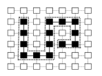
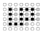
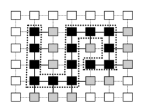
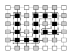
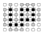
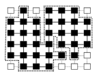
Figure 2: A demonstration of the barrier expansion process as a result of a contamination spread.

The robots’ goal is to clean $G$ by eliminating the contamination entirely.

It is important to note that no central control is allowed, and that the system is fully decentralized (i.e. all robots are identical and no explicit communication between the robots is allowed). An important advantage of this approach, in addition to the simplicity of the robots, is fault-tolerance — even if almost all the robots die and evaporate before completion, the remaining ones will eventually complete the mission, if possible.

A Survey of Previous Results. The cooperative cleaners problem was previously studied in (49) (static version) and (50, 51) (dynamic version). A cleaning algorithm called SWEEP was proposed (used by a decentralized group of simple mobile robots, for exploring and cleaning an unknown “contaminated” sub-grid $F$, expanding every $d$ time steps) and its performance analyzed.

The SWEEP algorithm is based in a constant traversal of the contaminated region, preserving the connectivity of the region while cleaning all non critical points — points which when cleaned disconnect the contaminated region. Using this algorithm the agents are guaranteed to stop only upon completing their mission. The algorithm can be implemented using only local knowledge, and local interactions by immediately adjacent agents. At each time step, each agent cleans its current location (assuming it is not a critical point), and moves according to a local movement rule, creating the effect of a clockwise “sweeping” traversal along the boundary of the contaminated region. As a result, the agents “peel” layers from the region, while preserving its connectivity, until the region is cleaned entirely. An illustration of two agents working according to the protocol can be seen in Figure 3.

Figure 3: An example of two agents using the SWEEP protocol, at time step 40 (with contamination spreading speed $d>40$). All the tiles presented were contaminated at time 0. The black dot denotes the starting point of the agents. The X’s mark the critical points which are not cleaned. The black tiles are the tiles cleaned by the first agent. The second layer of marked tiles represent the tiles cleaned by the second agent.

In order to formally describe the SWEEP algorithm, we should first define several additional terms. Let $\tau(t)=\big{(}\tau_{1}(t),\tau_{2}(t),\ldots,\tau_{k}(t)\big{)}$ denote the locations of the $k$ agents at time $t$. In addition, let $\tilde{\tau_{i}}(t)$ denote the “previous location” of agent $i$. Namely, the last tile that agent $i$ had been at, which is different than $\tau_{i}(t)$. This is formally defined as :

$$\tilde{\tau_{i}}(t)\triangleq\tau_{i}(x)\emph{ s.t. }x=\max\{j\in\mathbb{N}\ |\ j<t\emph{ and }\tau_{i}(j)\neq\tau_{i}(t)\}$$

The term $\partial F$ denotes the boundary of $F$, defined via :

$$\partial F=\{v\ |\ v\in F\ \wedge\ 8-Neighbors(v)\ \cap\ (G\ \setminus\ F)\ \neq\ \emptyset\}$$

The term ‘rightmost’ can now be defined as follows :

• If $t=0$ then select the tile as instructed in Figure 4.

• If $\tilde{\tau_{i}}(t)\in\partial F_{t}$ then starting from $\tilde{\tau_{i}}(t)$ (namely, the previous boundary tile that the agent had been in) scan the four neighbors of $\tau_{i}(t)$ in a clockwise order until a boundary tile (excluding $\tilde{\tau_{i}}(t)$) is found.

• If not $\tilde{\tau_{i}}(t)\in\partial F_{t}$ then starting from $\tilde{\tau_{i}}(t)$ scan the four neighbors of $\tau_{i}(t)$ in a clockwise order until the second boundary tile is found.

Figure 4: When $t=0$ the first movement of an agent located in $(x,y)$ should be decided according to initial contamination status of the neighbors of $(x,y)$, as appears in these charts — the agent’s initial location is marked with a filled circle while the destination is marked with an empty one. All configurations which do not appear in these charts can be obtained by using rotations. This definition is needed in order to initialize the traversal behavior of the agents in the correct direction.

A schematic flowchart of the protocol, describing its major components and procedures is presented in Figure 5. The complete pseudo-code of the protocol and its sub-routines appears in Figures 6 and 7. Upon initialization of the system, the System Initialization procedure is called (defined in Figure 6). This procedure sets various initial values of the agents, and calls the protocol’s main procedure — SWEEP (defined in Figure 7). This procedure in turn, uses various sub-routines and functions, all defined in Figure 6. The SWEEP procedure is comprised of a loop which is executed continuously, until detecting one of two possible break conditions. The first, implemented in the Check Completion of Mission procedure, is in charge of detecting cases where all the contaminated tiles have been cleaned. The second condition, implemented in the Check Near Completion of Mission procedure, is in charge of detecting scenarios in which every contaminated tile contains at least a single agent. In this case, the next operation would be a simultaneous cleaning of the entire contaminated tiles. Until these conditions are met, each agent goes through the following sequence of commands. First each agent calculates its desired destination at the current turn. Then, each agent calculated whether it should give a priority to another agent located at the same tile, and wishes to move to the same destination. When two or more agents are located at the same tile, and wish to move towards the same direction, the agent who had entered the tile first gets to leave the tile, while the other agents wait. In case several agents had entered the tile at the same time, the priority is determined using the Priority function. Before actually moving, each agent who had obtained a permission to move, must now locally synchronize its movement with its neighbors, in order to avoid simultaneous movements which may damage the connectivity of the region. This is done using the waiting dependencies mechanism, which is implemented by each agent via an internal positioning of itself in a local ordering of his neighboring agents. When an agent is not delayed by any other agent, it executes its desired movement. It is important to notice that at any given time, waiting or resting agents may become active again, if the conditions which made them become inactive in the first place, had changed.

Figure 5: A schematic flow chart of the SWEEP protocol. The smooth lines represent the basic flow of the protocol while the dashed lines represent cases in which the flow is interrupted. Such interruptions occur when an agent calculates that it must not move until other agents do so (either as a result of waiting or resting dependencies — see lines 6 and 14 of SWEEP for more details).

1: System Initialization

2:       Arbitrarily choose a pivot point $p_{0}$ in $\partial F_{0}$, and mark it as critical point

3:       Place all the agents on $p_{0}$

4:       For ($i=1$; $i\leq k$; $i++$) do

5:             Call Agent Reset for agent i

6:             Call SWEEP for agent i

7:             Wait two time steps

8:       End for

9: End procedure  

10: Agent Reset

11:       resting $\leftarrow$ false

12:       dest $\leftarrow$ null /* destination */

13:       near completion $\leftarrow$ false

14:       saturated perimeter $\leftarrow$ false

15:       waiting $\leftarrow$ $\emptyset$

16: End procedure  

17: Priority

18:       /* Assuming the agent moved from $(x_{0},y_{0})$ to $(x_{1},y_{1})$ */

19:       priority $\leftarrow$ $2(x_{1}-x_{0})+(y_{1}-y_{0})$

20: End procedure  

21: Check Completion of Mission

22:      If ($(x,y)=p_{0}$) and $(x,y)$ has no contaminated neighbors then

23:            If $(x,y)$ is contaminated then

24:                 Clean $(x,y)$

25:            STOP

26: End procedure  

27: Check “Near Completion” of Mission

28:       /* Cases where every tile in $F_{t}$ contains at least a single agent */

29:       near completion $\leftarrow$ false

30:       If each of the contaminated neighbors of (x,y) contains at least one agent then

31:            near completion $\leftarrow$ true

32:       If each of the contaminated neighbors of (x,y) satisfies near completion then

33:            Clean $\left(x,y\right)$ and STOP

34:       /* Cases where every non-critical tile in $\partial F_{t}$ contains at least 2 agents */

35:       saturated perimeter $\leftarrow$ false

36:       If $\left(\left(x,y\right)\in\partial F_{t}\right)$ and both $\left(x,y\right)$ and all of its non-critical neighbors       in $\partial F_{t}$ contain at least two agents then

37:            saturated perimeter $\leftarrow$ true

38:       If $\left(\left(x,y\right)\in\partial F_{t}\right)$ and both $\left(x,y\right)$ and all of its neighbors in $\partial F_{t}$ has       saturated perimeter = true then

39:            Ignore resting commands for this time step

40: End procedure

Figure 6: The first part of the SWEEP cleaning protocol.

1: SWEEP Protocol /* Controls agent $i$ after Agent Reset */

2:     Check Completion of Mission

3:     Check “Near Completion” of Mission

4:     dest $\leftarrow$ rightmost neighbor of (x,y) /* Calculate destination */

5:     destination signal bits $\leftarrow$ dest /* Signaling the desired destination */

6:     /* Calculate resting dependencies (solves agents’ clustering problem) */

7:     From all agents in (x,y) except agent $i$ we define be the following groups:

8:         $K_{1}$ : Agents signaling towards dest which entered (x,y) before agent $i$

9:         $K_{2}$ : Agents signaling towards dest which entered (x,y) with agent $i$,               and with higher priority than this of agent $i$

10:     resting $\leftarrow$ false

11:     If ($K_{1}\neq\emptyset$) or ($K_{2}\neq\emptyset$) then

12:         resting $\leftarrow$ true

13:         If (current time-step $\mathcal{T}$ did not end yet) then jump to 4 Else jump to 30

14:     waiting $\leftarrow$ $\emptyset$ /* Waiting dependencies (agents synchronization) */

15:     Let active agent denote a non-resting agent which didn’t move in $\mathcal{T}$ yet

16:     If (x-1,y) $\in F_{t}$ contains an active agent then waiting $\leftarrow$ waiting $\cup$ {left}

17:     If (x,y-1) $\in F_{t}$ contains an active agent then waiting $\leftarrow$ waiting $\cup$ {down}

18:     If (x-1,y-1) $\in F_{t}$ contains an active agent then waiting $\leftarrow$ waiting $\cup$ {l-d}

19:     If (x+1,y-1) $\in F_{t}$ contains an active agent then waiting $\leftarrow$ waiting $\cup$ {r-d}

20:     If dest = right and (x+1,y) contains an active agent $j$, and dest${}_{j}\neq$ left, and     there are no other agents delayed by agent $i$ (i.e. (x-1,y) does not contain     active agent $l$ with dest${}_{l}=$right and no active agents in (x,y+1),(x+1,y+1),     (x-1,y+1), and (x+1,y) does not contain active agent $n$ with dest${}_{n}=$ left),     then (waiting $\leftarrow$ waiting $\cup$ {right}) and $\left(\emph{waiting}_{j}\leftarrow\emph{waiting}_{j}\setminus\{\emph{left}\}\right)$

21:     If dest = up and (x,y+1) contains an active agent $j$, and dest${}_{j}\neq$ down, and     there are no other agents delayed by agent $i$ (i.e. (x,y-1) does not contain     active agent $l$ with dest${}_{l}=$up and no active agents in (x+1,y),(x+1,y+1),     (x-1,y+1), and (x,y+1) does not contain active agent $n$ with dest${}_{n}=$ down),     then (waiting $\leftarrow$ waiting $\cup$ {up}) and $\left(\emph{waiting}_{j}\leftarrow\emph{waiting}_{j}\setminus\{\emph{down}\}\right)$

22:     If (waiting $\neq\emptyset$) then

23:         If ($\mathcal{T}$ has not ended yet) then jump to 4 Else jump to 30

24:     /* Decide whether or not (x,y) should be cleaned */

25:     If $\neg$ ((x,y) $\in\partial F_{t}$) or ((x,y) $\equiv p_{0}$) or (x,y) has 2 contaminated tiles in its     $4Neighbors{}$ which are not connected via a path of contaminated tiles from its     $8Neighbors$ then

26:         (x,y) is an internal point or a critical point and should not be cleaned

27:     Else

28:         Clean (x,y) if and only if it does not still contain other agents

29:     Move to dest

30:     Wait until $\mathcal{T}$ ends.

31:     Return to 2

Figure 7: The SWEEP cleaning protocol.

Following are several results that we will later use. While using these results, we note that completely cleaning a region is at least as strong as covering it, as the number of “uncovered” tiles at any given time can be modeled by the number of “contaminated” tiles, since the number of uncovered tiles in the original region to be explored is clearly upper bounded at all times by the number of remaining contaminated tiles that belong to this region.

Result 1.

(Cleaning a Non-Expanding Contamination) The time it takes for a group of $K$ robots using the SWEEP algorithm to clean a region $F$ of the grid is at most:

$$t_{static}\triangleq\frac{8(|\partial F_{0}|-1)\cdot(W(F_{0})+k)}{k}+2k$$

Here $W(F)$ denotes the depth of the region $F$ (the shortest path from some internal point in $F$ to its boundary, for the internal point whose shortest path is the longest) and as defined above, $\partial F$ denotes the boundary of $F$, defined via :

$$\partial F=\{v\ |\ v\in F\ \wedge\ 8-Neighbors(v)\ \cap\ (G\ \setminus\ F)\ \neq\ \emptyset\}$$

The term $8-Neighbors(v)$ is used to denote the eight tiles that tile $v$ is immediately surrounded by.

Result 2.

(Universal Lower Bound on Contaminated Area) Using any cleaning algorithm, the area at time $t$ of a contaminated region that expands every $d$ time steps can be recursively lower bounded, as follows :

$$S_{t+d}\geq S_{t}-d\cdot k+\left\lfloor 2\sqrt{2\cdot(S_{t}-d\cdot k)-1}\right\rfloor$$

Here $S_{t}$ denotes the area of the contaminated region at time $t$ (such that $S_{0}=n$).

Result 3.

(Upper Bound on Cleaning Time for SWEEP on Expanding Domains) For a group of $k$ robot using the SWEEP algorithm to clean a region $F$ on the grid, that expands every $d$ time steps, the time it takes the robots to clean $F$ is at most $d$ multiplied by the minimal positive value of the following two numbers :

$$\frac{(A_{4}-A_{1}A_{3})\pm\sqrt{(A_{1}A_{3}-A_{4})^{2}-4A_{3}(A_{2}-A_{1}-A_{1}A_{4})}}{2A_{3}}$$

where :

$$A_{1}=\frac{c_{0}+2-\gamma_{2}}{4}\ ,\ A_{2}=\frac{c_{0}+2+\gamma_{2}}{4}\ ,\ A_{3}=\frac{8\cdot\gamma_{2}}{d\cdot k}\ ,\$$

$$A_{4}=\gamma_{1}-\frac{\gamma_{2}\cdot\gamma}{d}\ \ ,\ \ \gamma_{1}=\psi\left(1+A_{2}\right)-\psi\left(1+A_{1}\right)\$$

$$\gamma_{2}=\sqrt{(c_{0}+2)^{2}-8S_{0}+8}$$

$$\gamma=\frac{8(k+W(F_{0}))}{k}-\frac{d-2k}{|\partial F_{0}|-1}$$

Here $c_{0}$ is the circumference of the initial region $F_{0}$, and where $\psi(x)$ is the Digamma function (studied in (70)) — the logarithmic derivative of the Gamma function, defined as :

$$\psi(x)=\frac{d}{dx}\ln\Gamma(x)=\frac{\Gamma^{\prime}(x)}{\Gamma(x)}$$

or as :

$$\psi(x)=\int_{0}^{\infty}\left(\frac{e^{-t}}{t}-\frac{e^{-xt}}{1-e^{-t}}\right)\,dt$$

Note that although $c_{0}=O(|\partial F|)$ the actual length of the perimeter of the region can be greater than its cardinality, as several tiles may be traversed more than once. In fact, in (49) it is shown that $c_{0}\leq 2\cdot|\partial F|-2$.

4 Grid Coverage — Analysis

We note again that when discussing the coverage of regions on the grid, either static or expanding, it is enough to show that the region can be cleaned by the team of robots, as clearly the cleaned sites are always a subset of the visited ones. We first present the cover time of a group of robots operating in non-expanding domains, using the SWEEP algorithm.

Theorem 1.

Given a connected region of $S_{0}=n$ grid tiles and perimeter $c_{0}$, that should be covered by a team of $k$ ant-like robots, the robots can cover it using $O\left(\frac{1}{k}S_{0}^{1.5}+S_{0}\right)$ time.

Proof.

Since $|\partial F_{0}|=\Theta(c_{0})$, and $W(F_{0})=O(\sqrt{S_{0}})$, recalling Result 1 we can see that :

$$t_{k}(n)=t_{static}(k)=O\left(\frac{1}{k}\sqrt{S_{0}}\cdot c_{0}+c_{0}+k\right)$$

As $c_{0}=O(S_{0})$ and as for practical reasons we assume that $k<n$ this would equal in the worse case to :

$$t_{k}(n)=t_{static}(k)=O\left(\frac{1}{k}S_{0}^{1.5}+S_{0}\right)$$

∎

We now examine the problem of covering expanding domains. The lower bound for the number of robots required for completing is as follows.

Theorem 2.

Given a region of size $S_{0}\geq 3$ tiles, expanding every $d$ time steps, then a team of less than $\frac{\sqrt{S_{0}}}{d}$ robots cannot clean the region, regardless of the algorithm used.

Proof.

Recalling Result 2 we can see that :

$$S_{t+d}-S_{t}\geq\left\lfloor 2\sqrt{2\cdot(S_{t}-d\cdot k)-1}\right\rfloor-d\cdot k$$

By assigning $k=\frac{\sqrt{S_{0}}}{d}$ we can see that :

$$\Delta S_{t}=S_{t+d}-S_{t}\geq\left\lfloor 2\sqrt{2\cdot(S_{t}-\sqrt{S_{0}})-1}\right\rfloor-\sqrt{S_{0}}$$

For any $S_{0}\geq 3$, we see that $\Delta S_{0}>0$. In addition, for every $S_{0}\geq 3$ we can see that $\frac{dS_{t}}{dt}>0$ for every $t\geq 0$. Therefore, for every $S_{0}\geq 3$ the size of the region will be forever growing. ∎

Corollary 1.

Given a region of size $S_{0}$ tiles, expanding every $d$ time steps, where $d=O(1)$ w.r.t $S_{0}$, then a team of less than $\Omega(\sqrt{S_{0}})$ robots cannot clean the region, regardless of the algorithm used.

Theorem 3.

Given a region $F$ of size $S_{0}$ tiles, expanding every $d$ time steps, where $R(F)$ is the perimeter of the bounding rectangle of the region $F$, then a team of $k$ robots that at $t=0$ are located at the same tile cannot clean the region, regardless of the algorithm used, as long as $d^{2}k<\Omega(R(F))$.

Proof.

For every $v\in F$ let $l(v)$ denote the maximal distance between $v$ and any of the tiles of $F$, namely :

$$l(v)=\max\{d(v,u)|u\in F\}$$

Let $C(F)=l(v_{c})$ such that $v_{c}\in F$ is the tile with minimal value of $l(v)$.

Let $v_{s}$ denote the tile the agents are located in at $t=0$. Let $v_{d}\in F$ denote some contaminated tile such that $d(v_{s},v_{d})=l(v_{s})$. Regardless of the algorithm used by the agents, until some agent reaches $v_{d}$ there will pass at least $l(v_{s})$ time steps. Let us assume w.l.o.g that $v_{d}$ is located to the right (or of the same horizontal coordinate) and to the top (or of the same vertical coordinate) of $v_{s}$. Then by the time some agent is able to reach $v_{d}$ there exists an upper-right quarter of a digital sphere of radius $\left\lfloor\frac{l(v_{s})}{d}\right\rfloor+1$, whose center is $v_{d}$.

The number of tiles in such a quarter of digital sphere equals :

$$\frac{1}{2}\left\lfloor\frac{l(v_{s})}{d}\right\rfloor^{2}+\frac{3}{2}\left\lfloor\frac{l(v_{s})}{d}\right\rfloor+1=\Theta\left(\frac{l(v_{s})^{2}}{d^{2}}\right)$$

It is obvious that the region cannot be cleaned until $v_{d}$ is cleaned. Let $t_{d}$ denote the time at which the first agent reaches $v_{d}$. It is easy to see that $t_{d}\geq l(v_{s})$. Therefore, regardless of activities of the agents until time step $t_{d}$, there are now $k$ agents that has to clean a region of at least $\Theta\left(\frac{l(v_{s})^{2}}{d^{2}}\right)$ tiles, spreading every $d$ time steps. Using Theorem 2 we know that $k$ agents cannot clean an expanding region of $k=\frac{\sqrt{S_{0}}}{d}$ tiles. Namely, at time $t_{d}$ $k$ agents could not clean the contaminated tiles if :

$$d^{2}k<\Omega\left(l(v_{s})\right)$$

As $l(v_{s})\geq C(F)$ we know that $k$ agents could not clean an expanding contaminated region where : $d^{2}k<\Omega\left(C(F)\right)$. It is easy to see that for every region $F$, if $R(F)$ is the length of the perimeter of the bounding rectangle of $F$ then $C(F)=\Theta(R(F))$. ∎

Lemma 1.

For every connected region of size $S_{0}\geq 3$ and perimeter of length $c_{0}$ :

$$\frac{1}{2}c_{0}<\gamma_{2}<c_{0}$$

Proof.

let us assume by contradiction that $(c_{0}+2)^{2}\leq(8S_{0}+8)$. This means $c_{0}\leq\sqrt{8S_{0}+8}-2$. However, the minimal circumference of a region of size $S_{0}$ is achieved when the region is arranged in the form of an 8-connected digital sphere, in which case $c_{0}\geq 4\sqrt{S_{0}}-4$, contradicting the assumption that $c_{0}\leq\sqrt{8S_{0}+8}-2$ for every $S_{0}>5$. Therefore, $\gamma_{2}\in\mathbb{R}$.

Let us assume by contradiction that $\gamma_{2}<\frac{1}{2}c_{0}$. Therefore :

$$(c_{0}+2)^{2}-8S_{0}+8<\frac{1}{4}c_{0}^{2}$$

which implies :

$$c_{0}<-\frac{16}{6}+\sqrt{10\frac{2}{3}S_{0}-8\frac{8}{9}}<3.266\sqrt{S_{0}}-2$$

However, we know that $c_{0}\geq 4\sqrt{S_{0}}-4$, which contradicts the assumption that $\gamma_{2}<\frac{1}{2}c_{0}$ for every $S_{0}\geq 3$.

Let us assume by contradiction that $\gamma_{2}>c_{0}$. Therefore :

$$(c_{0}+2)^{2}-8S_{0}+8>c_{0}^{2}$$

which implies :

$$c_{0}>4S_{0}-6$$

However, we know that $c_{0}\leq 2S_{0}-2$ (as $c_{0}$ is maximized when the tiles are arranged in the form of a straight line), contradicting the assumption that $\gamma_{2}>c_{0}$ for every $S_{0}\geq 3$. ∎

Lemma 2.

For every connected region of size $S_{0}\geq 3$ and perimeter of length $c_{0}$ :

$$\Omega(1)<\gamma_{1}<O(\ln n)$$

Proof.

Let us observe $\gamma_{1}$ :

$$\gamma_{1}\triangleq\psi\left(1+\frac{c_{0}+2+\gamma_{2}}{4}\right)-\psi\left(1+\frac{c_{0}+2-\gamma_{2}}{4}\right)$$

From Lemma 1 we can see that $1<\left(1+\frac{c_{0}+2-\gamma_{2}}{4}\right)<\frac{1}{4}c_{0}$. Note that $\psi(1)=-\hat{\gamma}$ where $\hat{\gamma}$ is the Euler -Mascheroni constant, defined as :

$$\hat{\gamma}=\lim_{n\rightarrow\infty}\left[\left(\sum_{k=1}^{n}\frac{1}{k}\right)-\log(n)\right]=\int_{1}^{\infty}\left({1\over\lfloor x\rfloor}-{1\over x}\right)\,dx$$

which equals approximately $0.57721$. In addition, $\psi(x)$ is monotonically increasing for every $x>0$. As we also know that $\psi(x)$ is upper bounded by $O(\ln x)$ for large values of $x$, we see that :

$$-0.58<\psi\left(1+\frac{c_{0}+2-\gamma_{2}}{4}\right)<O(\ln n)$$ (4.1)

From Lemma 1 we also see that $1<\left(1+\frac{c_{0}+2+\gamma_{2}}{4}\right)<\frac{1.5}{4}c_{0}$ meaning that :

$$\psi\left(1+\frac{c_{0}+2+\gamma_{2}}{4}\right)=\Theta(\ln n)$$ (4.2)

Combining equations 4.1 and 4.2 we see that :

$$\Omega(1)<\gamma_{1}<O(\ln n)$$ (4.3)

∎

Theorem 4.

Result 3 returns a positive real number for the covering time of a region of $S_{0}$ tiles that expands every $d$ time steps, when the number of robots is $\Theta(\sqrt{S_{0}})$ and $d=\Omega(\frac{c_{0}}{\gamma_{1}})$, and where $\gamma_{1}$ shifts from $O(1)$ to $O(\ln S_{0})$ as $c_{0}$ grows from $O(\sqrt{S_{0}})$ to $O(S_{0})$, defined as :

$$\gamma_{1}=\psi\left(1+\frac{c_{0}+2+\gamma_{2}}{4}\right)-\psi\left(1+\frac{c_{0}+2-\gamma_{2}}{4}\right)$$

$$\gamma_{2}=\sqrt{(c_{0}+2)^{2}-8S_{0}+8}$$

Proof.

Following are the requirements that must hold in order for Result 3 to yield a real number :

• $d\cdot k\neq 0$

• $|\partial F|>1$

• $A_{3}\neq 0$

• $(c_{0}+2)^{2}>8S_{0}-8$

• $(A_{1}A_{3}-A_{4})^{2}\geq 4A_{3}(A_{2}-A_{1}-A_{1}A_{4})$

The first and second requirements hold for every non trivial scenario. The third requirement is implied by the fourth. The fourth assumption is a direct result of Lemma 1.

As for the last requirement, we ask that :

$$A_{1}^{2}A_{3}^{2}+A_{4}^{2}\geq 4A_{2}A_{3}-4A_{1}A_{3}-2A_{1}A_{3}A_{4}$$

which subsequently means that we must have :

$$\begin{array}[]{c}\frac{\gamma_{2}^{2}}{d^{2}k^{2}}\left(c_{0}^{2}+\gamma_{2}^{2}-c_{0}\gamma_{2}\right)\\ +\gamma_{1}^{2}+\frac{\gamma_{2}^{2}\gamma^{2}}{d}-\frac{\gamma\gamma_{1}\gamma_{2}}{d}\end{array}\geq 4\frac{\gamma_{2}}{dk}\left(\begin{array}[]{c}4\gamma_{2}-c_{0}\gamma_{1}+\\ c_{0}\frac{\gamma_{2}\gamma}{d}-2\gamma_{1}+2\frac{\gamma_{2}\gamma}{d}+\\ \gamma_{1}\gamma_{2}-\frac{\gamma_{2}^{2}\gamma}{d}\end{array}\right)$$

Using Lemma 1 and Lemma 2 we should make sure that :

$$\frac{\gamma_{2}^{2}}{dk^{2}}c_{0}^{2}+\gamma_{1}^{2}d+\gamma_{2}^{2}\gamma^{2}-\gamma\gamma_{1}\gamma_{2}\geq O\left(\frac{c_{0}\gamma_{2}\gamma_{1}}{k}+\frac{c_{0}\gamma_{2}^{2}\gamma}{dk}\right)$$

Using $W(F)=O(\sqrt{S_{0}})$ and $\Omega(\sqrt{S_{0}})=|\partial F|=O(S_{0})$ and dividing by $\gamma_{2}^{2}$ (which we know to be larger than zero), we can write the above as follows :

$$\frac{c_{0}^{2}}{dk^{2}}+\frac{k^{2}+d\ln^{2}S_{0}}{c_{0}^{2}}+1\geq$$

$$O\left(\frac{\ln S_{0}}{c_{0}}+\frac{k\ln S_{0}}{c_{0}^{2}}+\frac{\ln S_{0}}{k}+\frac{c_{0}\sqrt{S_{0}}}{dk^{2}}+\frac{c_{0}}{dk}+\frac{1}{d}\right)$$

As $c_{0}\geq\sqrt{S_{0}}$ then $\frac{c_{0}^{2}}{dk^{2}}\geq\frac{c_{0}\sqrt{S_{0}}}{dk^{2}}$. In addition, $1\geq\frac{1}{d}$ and also $1\geq\frac{\ln S_{0}}{c_{0}}$ and $1\geq\frac{\ln S_{0}}{k}$ (as Eq. 4.6 shows that $k\geq\ln S_{0}$). In order to have also $1\geq\frac{c_{0}}{dk}$ we must have :

$$d\cdot k=\Omega(c_{0})$$ (4.4)

In addition, we should also require that the result $\mu$ would be positive (as it denotes the coverage time). Namely, that :

$$A_{4}+\sqrt{(A_{1}A_{3}-A_{4})^{2}-4A_{3}(A_{2}-A_{1}-A_{1}A_{4})}>A_{1}A_{3}$$

For this to hold we shall merely require that:

$$A_{2}-A_{1}-A_{1}A_{4}\leq 0$$

(as $A_{3}$ is known to be positive). Assigning the values of $A_{1},A_{2},A_{4}$, this translates to :

$$c_{0}+c_{0}^{2}\frac{\gamma}{d}\leq O(c_{0}\gamma_{1})$$

Dividing by $c_{0}$ we can write :

$$1+c_{0}\frac{1+\frac{\sqrt{S_{0}}}{k}-\frac{d}{c_{0}}+\frac{k}{c_{0}}}{d}\leq O(\gamma_{1})$$

Namely :

$$c_{0}+\frac{c_{0}\sqrt{S_{0}}}{k}+k\leq dO(\gamma_{1})$$

As $c_{0}$ is the dominant element of the left side of the inequation, we see that :

$$d=\Omega\left(\frac{c_{0}}{\gamma_{1}}\right)$$ (4.5)

Assigning this lower bound for $d$ we can now see that :

$$\Omega(\sqrt{S_{0}})\leq k\leq O(c_{0})$$ (4.6)

Therefore, we shall select the value of $k$ such that :

$$k=\Theta(\sqrt{S_{0}})$$

This also satisfies Equation 4.4. ∎

Theorem 5.

The time it takes a group of $k=\Theta(\sqrt{S_{0}})$ robots using the SWEEP algorithm to cover a connected region of size $S_{0}$ tiles, that expands every $d=\Omega(\frac{c_{0}}{\gamma_{1}})$ time steps, is upper bounded as follows :

$$t_{SUCCESS}=O\left(S_{0}^{2}\ln S_{0}\right)$$

where $\gamma_{1}$ shifts from $O(1)$ to $O(\ln S_{0})$ as $c_{0}$ grows from $O(\sqrt{S_{0}})$ to $O(S_{0})$, defined as :

$$\gamma_{1}=\psi\left(1+\frac{c_{0}+2+\gamma_{2}}{4}\right)-\psi\left(1+\frac{c_{0}+2-\gamma_{2}}{4}\right)$$

$$\gamma_{2}=\sqrt{(c_{0}+2)^{2}-8S_{0}+8}$$

Proof.

Recalling Result 1 we know that if :

$$\frac{8(|\partial F_{0}|-1)\cdot(W(F_{0})+k)}{k}+2k<d$$

then the robots could clean the region before it expands even once. In this case, the cleaning time would be $O(\frac{1}{k}\sqrt{S_{0}}\cdot c_{0}+c_{0})$ as was shown in Theorem 1. Therefore, we shall assume that :

$$\frac{8(|\partial F_{0}|-1)\cdot(W(F_{0})+k)}{k}+2k\geq d$$ (4.7)

Observing Result 3 we see that :
$t_{SUCCESS}=$

$$d\cdot O\left(A_{1}+\frac{|A_{4}|}{A_{3}}+\sqrt{A_{1}^{2}+\frac{|A_{1}A_{4}|+A_{1}+A_{2}}{A_{3}}+\frac{A_{4}^{2}}{A_{3}^{2}}}\right)\leq$$

$$d\cdot O\left(A_{1}+\frac{|A_{4}|}{A_{3}}+\frac{\sqrt{A_{3}}\sqrt{|A_{1}A_{4}|+A_{1}+A_{2}}}{A_{3}}+\frac{|A_{4}|}{A_{3}}\right)\leq$$

$$d\cdot O\left(A_{1}+\frac{|A_{4}|}{A_{3}}+\frac{\sqrt{|A_{1}A_{4}|}+\sqrt{A_{1}}+\sqrt{A_{2}}}{\sqrt{A_{3}}}\right)=$$

$$d\cdot O\left(\begin{array}[]{c}c_{0}+\gamma_{2}+dk\frac{\gamma_{1}}{\gamma_{2}}+k\gamma+\\ \sqrt{k}\frac{\sqrt{c_{0}+\gamma_{2}}\sqrt{d\gamma_{1}+\gamma_{2}\cdot\gamma}}{\sqrt{\gamma_{2}}}+\sqrt{\frac{kd}{\gamma_{2}}}\sqrt{c_{0}+\gamma_{2}}\end{array}\right)$$

Using the fact that $\gamma_{2}=\Theta(c_{0})$ (Lemma 1) we can rewrite this expression as :

$$d\cdot O\left(c_{0}+dk\frac{\gamma_{1}}{c_{0}}+k\gamma+\sqrt{k}\sqrt{d\gamma_{1}+c_{0}\gamma}+\sqrt{kd}\right)$$ (4.8)

Recalling Equation 4.7, and as $W(F_{0})=O(\sqrt{S_{0}})$, we can see that :

$$d=O\left(\frac{\sqrt{S_{0}}\cdot c_{0}}{k}+c_{0}+k\right)$$

Therefore, $|\gamma|$ can now be written as :

$$|\gamma|=O\left(\frac{\sqrt{S_{0}}}{k}+\sqrt{S_{0}}+\frac{k}{\sqrt{S_{0}}}+1\right)$$

In addition, remembering that $O(\sqrt{S_{0}})\leq c_{0}\leq O(S_{0})$ we can rewrite the expression of Equation 4.8 as follows :

$$d\cdot O\left(\begin{array}[]{c}c_{0}+dk\frac{\gamma_{1}}{c_{0}}+k\sqrt{S_{0}}+\frac{k^{2}}{\sqrt{S_{0}}}+\\ \sqrt{kc_{0}}\sqrt{\frac{d}{c_{0}}\gamma_{1}+\frac{\sqrt{S_{0}}}{k}+\sqrt{S_{0}}+\frac{k}{\sqrt{S_{0}}}}+\sqrt{kd}\end{array}\right)=$$

$$d\cdot O\left(\begin{array}[]{c}c_{0}+dk\frac{\gamma_{1}}{c_{0}}+k\sqrt{S_{0}}+\frac{k^{2}}{\sqrt{S_{0}}}+\\ \sqrt{kc_{0}}\left(\sqrt{\gamma_{1}}+\sqrt[4]{S_{0}}\sqrt{\frac{\gamma_{1}}{k}}+\sqrt[4]{S_{0}}+\frac{\sqrt{k}}{\sqrt[4]{S_{0}}}\right)+\sqrt{kd}\end{array}\right)$$

Using Lemma 2 we see that :

$$d\cdot O\left(\begin{array}[]{c}c_{0}+dk\frac{\ln S_{0}}{c_{0}}+k\sqrt{S_{0}}+\frac{k^{2}}{\sqrt{S_{0}}}+\\ \sqrt{c_{0}\ln S_{0}\sqrt{S_{0}}}+\sqrt{c_{0}k\sqrt{S_{0}}}+k\sqrt[4]{S_{0}}+\sqrt{kd}\end{array}\right)=$$

$$d\cdot O\left(\begin{array}[]{c}c_{0}+k\sqrt{S_{0}}\ln S_{0}+\frac{k^{2}}{\sqrt{S_{0}}}+\\ \sqrt{c_{0}\ln S_{0}\sqrt{S_{0}}}+\sqrt{c_{0}k\sqrt{S_{0}}}\end{array}\right)$$ (4.9)

Assuming that $k>O(\ln S_{0})$ and as $c_{0}=O(S_{0})$ we can now write :

$$O\left(\begin{array}[]{c}\frac{S_{0}^{2.5}}{k}+S_{0}^{2}\ln S_{0}+S_{0}^{1.5}k\ln S_{0}+k^{2}\sqrt{S_{0}}\ln S_{0}+\\ \frac{k^{3}}{\sqrt{S_{0}}}+\frac{S_{0}^{2.25}}{\sqrt{k}}+S_{0}^{1.75}\sqrt{k}+S_{0}^{0.75}k^{1.5}\end{array}\right)$$ (4.10)

Using Equation 4.6 we can see that this translates to :

$$O\left(S_{0}^{1.5}k\ln S_{0}\right)$$ (4.11)

∎

5 Conclusions

In this paper we have discussed the problem of cleaning or covering a connected region on the grid using a collaborate team of simple, finite-state-automata robotic agents. We have shown that when the regions are static, this can be done in $O(\frac{1}{k}\sqrt{n}\cdot c_{0}+c_{0}+k)$ time which equals $O(\frac{1}{k}n^{1.5}+n)$ time in the worst case, thus improving the previous results for this problem. In addition, we have shown that when the region is expanding in a constant rate (which is “slow enough”), a team of $\Theta(\sqrt{n})$ robots can still be guaranteed to clean or cover it, in $O(n^{2}\ln n)$ time.

In addition, we have shown that teams of less than $\Omega(\sqrt{n})$ robots can never cover a region that expands every $O(1)$ time steps, regardless of their sensing capabilities, communications and memory resources employed, or the algorithm used. As to regions that expand slower than every $O(1)$ time steps, we have shown the following impossibility results. First, a region of $n$ tiles that expands every $d$ time steps cannot be covered by a group of $k$ agents if $dk\leq O(\sqrt{n})$. Using Theorem 4 we can guarantee a coverage when $dk=\Omega(\frac{n^{1.5}}{\ln n})$, or even for $dk=\Omega(n))$ (when the region’s perimeter $c_{0}$ equals $O(n)$).

Second, a spreading region cannot be covered when $d^{2}k$ is smaller than the order of the perimeter of the bounding rectangle of the region (which equals $O(n)$ in the worse case and $O(\sqrt{n})$ for shapes with small perimeters). Using Theorem 4 we can guarantee a coverage when $d^{2}k=\Omega(\frac{n^{2.5}}{\ln^{2}n})$, or for $d^{2}k=\Omega(n^{1.5})$ (when the region’s perimeter $c_{0}$ equals $O(n)$).

We believe that these results can be easily applied to various other problems in which a team of agents are required to operate in an expanding grid domain. For example, this result can show that a team of $\Theta(\sqrt{n})$ cops can always catch a robber (or for that matter — a group of robbers), moving (slowly) in an unbounded grid. Alternatively, robbers can be guaranteed to escape a team of less than $O(\sqrt{n})$ cops, if the area they are located in is unbounded.

6 Vitae

	Dr. Altshuler received his PhD in Computer Science from the Technion — Israel Institute of Technology (2009), and is now a post-doc researcher at the Deutsche Telekom Research Lab in Ben Gurion University.
	Prof. Bruckstein is a professor at the Computer Science department at the Technion — Israel Institute of Technology, received his PhD in Electrical Engineering from Stanford University (1984).

References

- (1) S. Mastellone, D. Stipanovi, C. Graunke, K. Intlekofer, M. Spong, Formation control and collision avoidance for multi-agent non-holonomic systems: Theory and experiments, The International Journal of Robotics Research 27 (1) (2008) 107–126.
- (2) S. DeLoach, M. Kumar, Intelligence Integration in Distributed Knowledge Management, Idea Group Inc (IGI), 2008, Ch. Multi-Agent Systems Engineering: An Overview and Case Study, pp. 207– 224.
- (3) I. Wagner, A. Bruckstein, From ants to a(ge)nts: A special issue on ant—robotics, Annals of Mathematics and Artificial Intelligence, Special Issue on Ant Robotics 31 (1–4) (2001) 1–6.
- (4) U. V. et. al, RoboCup 2007: Robot Soccer World Cup XI, Vol. 5001 of Lecture Notes in Computer Science, Springer Berlin, 2008.
- (5) R. Alami, S. Fleury, M. Herrb, F. Ingrand, F. Robert, Multi-robot cooperation in the martha project, IEEE Robotics and Automation Magazine 5 (1) (1998) 36–47.
- (6) N. Agmon, S. Kraus, G. Kaminka, Multi-robot perimeter patrol in adversarial settings, in: IEEE International Conference on Robotics and Automation (ICRA 2008), 2008, pp. 2339–2345.
- (7) N. Agmon, V. Sadov, G. Kaminka, S. Kraus, The impact of adversarial knowledge on adversarial planning in perimeter patrol, in: AAMAS ’08: Proceedings of the 7th international joint conference on Autonomous agents and multiagent systems, International Foundation for Autonomous Agents and Multiagent Systems, Richland, SC, 2008, pp. 55–62.
- (8) S. Kraus, O. Shehory, G. Taase, Coalition formation with uncertain heterogeneous information, in: Proceedings of the second international joint conference on Autonomous agents and multiagent systems, 2003, pp. 1–8.
- (9) H. Work, E. Chown, T. Hermans, J. Butterfield, Robust team-play in highly uncertain environments, in: AAMAS ’08: Proceedings of the 7th international joint conference on Autonomous agents and multiagent systems, International Foundation for Autonomous Agents and Multiagent Systems, Richland, SC, 2008, pp. 1199–1202.
- (10) M. Rehak, M. Pechoucek, P. Celeda, V. Krmicek, M. Grill, K. Bartos, Multi-agent approach to network intrusion detection, in: AAMAS ’08: Proceedings of the 7th international joint conference on Autonomous agents and multiagent systems, International Foundation for Autonomous Agents and Multiagent Systems, Richland, SC, 2008, pp. 1695–1696.
- (11) R. Connaughton, P. Schermerhorn, M. Scheutz, Physical parameter optimization in swarms of ultra-low complexity agents, in: AAMAS ’08: Proceedings of the 7th international joint conference on Autonomous agents and multiagent systems, International Foundation for Autonomous Agents and Multiagent Systems, Richland, SC, 2008, pp. 1631–1634.
- (12) M. Mataric, Interaction and intelligent behavior, Ph.D. thesis, Massachusetts Institute of Technology (1994).
- (13) E. Manisterski, R. Lin, S. Kraus, Understanding how people design trading agents over time, in: AAMAS ’08: Proceedings of the 7th international joint conference on Autonomous agents and multiagent systems, International Foundation for Autonomous Agents and Multiagent Systems, Richland, SC, 2008, pp. 1593–1596.
- (14) D. MacKenzie, R. Arkin, J. Cameron, Multiagent mission specification and execution, Autonomous Robots 4 (1) (1997) 29–52.
- (15) G. Chalkiadakis, C. Boutilier, Sequential decision making in repeated coalition formation under uncertainty, in: Proceedings of the 7th international joint conference on Autonomous agents and multiagent systems, 2008, pp. 347–354.
- (16) X. Zheng, S. Koenig, Reaction functions for task allocation to cooperative agents, in: Proceedings of the 7th international joint conference on Autonomous agents and multiagent systems, 2008, pp. 559–566.
- (17) C. Candea, H. Hu, L. Iocchi, D. Nardi, M. Piaggio, Coordinating in multi-agent robocup teams, Robotics and Autonomous Systems 36 (2–3) (2001) 67–86.
- (18) R. Sawhney, K. Krishna, K. Srinathan, M. Mohan, On reduced time fault tolerant paths for multiple uavs covering a hostile terrain, in: AAMAS ’08: Proceedings of the 7th international joint conference on Autonomous agents and multiagent systems, International Foundation for Autonomous Agents and Multiagent Systems, Richland, SC, 2008, pp. 1171–1174.
- (19) A. Yamashita, M. Fukuchi, J. Ota, T. Arai, H. Asama, Motion planning for cooperative transportation of a large object by multiple mobile robots in a 3d environment, in: In Proceedings of IEEE International Conference on Robotics and Automation, 2000, pp. 3144–3151.
- (20) A. Agogino, K. Tumer, Regulating air traffic flow with coupled agents, in: AAMAS ’08: Proceedings of the 7th international joint conference on Autonomous agents and multiagent systems, International Foundation for Autonomous Agents and Multiagent Systems, Richland, SC, 2008, pp. 535–542.
- (21) S. Premvuti, S. Yuta, Consideration on the cooperation of multiple autonomous mobile robots, in: Proceedings of the IEEE International Workshop of Intelligent Robots and Systems, 1990, pp. 59–63.
- (22) R. Bhatt, C. Tang, V. Krovi, Formation optimization for a fleet of wheeled mobile robots a geometric approach, Robotics and Autonomous Systems 57 (1) (2009) 102–120.
- (23) J. Fredslund, M. Mataric, Robot formations using only local sensing and control, in: Proceedings of the International Symposium on Computational Intelligence in Robotics and Automation (IEEE CIRA 2001), 2001, pp. 308–313.
- (24) N. Gordon, I. Wagner, A. Bruckstein, Discrete bee dance algorithms for pattern formation on a grid, in: IEEE International Conference on Intelligent Agent Technology (IAT03), 2003, pp. 545–549.
- (25) K. Bendjilali, F. Belkhouche, B. Belkhouche, Robot formation modelling and control based on the relative kinematics equations, The International Journal of Robotics and Automation 24 (1) (2009) 3220–.
- (26) T. Balch, R. Arkin, Behavior-based formation control for multi-robot teams, IEEE Transactions on Robotics and Automation 14 (6) (1998) 926–939.
- (27) S. Sariel, T. Balch, Real time auction based allocation of tasks for multi-robot exploration problem in dynamic environments, in: In Proceedings of the AAAI-05 Workshop on Integrating Planning into Scheduling, 2005, pp. 27–33.
- (28) M. Pfingsthorn, B. Slamet, A. Visser, RoboCup 2007: Robot Soccer World Cup XI, Vol. 5001 of Lecture Notes in Computer Science, Springer Berlin, 2008, Ch. A Scalable Hybrid Multi-robot SLAM Method for Highly Detailed Maps, pp. 457–464.
- (29) I. Rekleitis, G. Dudek, E. Milios, Experiments in free-space triangulation using cooperative localization, in: IEEE/RSJ/GI International Conference on Intelligent Robots and Systems (IROS), 2003.
- (30) I. Harmatia, K. Skrzypczykb, Robot team coordination for target tracking using fuzzy logic controller in game theoretic framework, Robotics and Autonomous Systems 57 (1) (2009) 75–86.
- (31) L. Parker, C. Touzet, Multi-robot learning in a cooperative observation task, Distributed Autonomous Robotic Systems 4 (2000) 391–401.
- (32) G. Hollinger, S. Singh, J. Djugash, A. Kehagias, Efficient multi-robot search for a moving target, The International Journal of Robotics Research 28 (2) (2009) 201–219.
- (33) S. LaValle, D. Lin, L. Guibas, J. Latombe, R. Motwani, Finding an unpredictable target in a workspace with obstacles, in: Proceedings of the 1997 IEEE International Conference on Robotics and Automation (ICRA-97), 1997, pp. 737–742.
- (34) A. Efraim, D.Peleg, Distributed algorithms for partitioning a swarm of autonomous mobile robots, Structural Information and Communication Complexity, Lecture Notes in Computer Science 4474 (2007) 180–194.
- (35) R. Olfati-Saber, Flocking for multi-agent dynamic systems: Algorithms and theory, IEEE Transactions on Automatic Control 51 (3) (2006) 401–420.
- (36) E. Bonabeau, M. Dorigo, G. Theraulaz, Swarm Intelligence: From Natural to Artificial Systems, Oxford University Press, US, 1999.
- (37) G. Beni, J. Wang, Theoretical problems for the realization of distributed robotic systems, in: IEEE Internal Conference on Robotics and Automation, 1991, pp. 1914–1920.
- (38) A. Thorndike, Summary of antisubmarine warfare operations in world war ii, Summary report, NDRC Summary Report (1946).
- (39) P. Morse, G. Kimball, Methods of operations research, MIT Press and New York: Wiley, 1951.
- (40) B. Koopman, Search and Screening: General Principles with Historical Applications, Pergamon Press, 1980.
- (41) P. Vincent, I. Rubin, A framework and analysis for cooperative search using uav swarms, in: ACM Simposium on applied computing, 2004.
- (42) Y. Altshuler, V. Yanovsky, A. Bruckstein, I. Wagner, Efficient cooperative search of smart targets using uav swarms, ROBOTICA 26 (2008) 551–557.
- (43) S. Koenig, M. Likhachev, X. Sun, Speeding up moving-target search, in: AAMAS ’07: Proceedings of the 6th international joint conference on Autonomous agents and multiagent systems, ACM, New York, NY, USA, 2007, pp. 1–8.
- (44) R. Borie, C. Tovey, S. Koenig, Algorithms and complexity results for pursuit-evasion problems, In Proceedings of the International Joint Conference on Artificial Intelligence (IJCAI) (2009) 59–66.
- (45) R. Isaacs, Differential Games: A Mathematical Theory with Applications to Warfare and Pursuit, Control and Optimization, John Wiley and Sons, Reprinted by Dover Publications 1999, 1965.
- (46) V. Isler, S. Kannan, S. Khanna, Randomized pursuit-evasion with local visibility, SIAM Journal of Discrete Mathematics 20 (2006) 26–41.
- (47) A. Goldstein, E. Reingold, The complexity of pursuit on a graph, Theoretical Computer Science 143 (1995) 93–112.
- (48) J. Flynn, Lion and man: the general case, SIAM Journal of Control 12 (1974) 581–597.
- (49) I. Wagner, Y. Altshuler, V. Yanovski, A. Bruckstein, Cooperative cleaners: A study in ant robotics, The International Journal of Robotics Research (IJRR) 27 (1) (2008) 127–151.
- (50) Y. Altshuler, A. Bruckstein, I. Wagner, Swarm robotics for a dynamic cleaning problem, in: IEEE Swarm Intelligence Symposium, 2005, pp. 209–216.
- (51) Y. Altshuler, I. Wagner, A. Bruckstein, Swarm ant robotics for a dynamic cleaning problem — upper bounds, The 4th International conference on Autonomous Robots and Agents (ICARA-2009) (2009) 227–232.
- (52) V. Braitenberg, Vehicles, MIT Press, 1984.
- (53) R. Korf, Real-time heuristic search, Artificial Intelligence 42 (1990) 189–211.
- (54) I. Rekleitis, V. Lee-Shuey, A. P. Newz, H. Choset, Limited communication, multi-robot team based coverage, in: IEEE International Conference on Robotics and Automation, 2004.
- (55) Z. Butler, A. Rizzi, R. Hollis, Distributed coverage of rectilinear environments, in: Proceedings of the Workshop on the Algorithmic Foundations of Robotics, 2001.
- (56) E. Acar, Y. Zhang, H. Choset, M. Schervish, A. Costa, R. Melamud, D. Lean, A. Gravelin, Path planning for robotic demining and development of a test platform, in: International Conference on Field and Service Robotics, 2001, pp. 161–168.
- (57) M. Batalin, G. Sukhatme, Spreading out: A local approach to multi-robot coverage, in: 6th International Symposium on Distributed Autonomous Robotics Systems, 2002.
- (58) X. Zheng, S. Koenig, Robot coverage of terrain with non-uniform traversability, in: In Proceedings of the IEEE International Conference on Intelligent Robots and Systems (IROS), 2007, pp. 3757–3764.
- (59) X. Zheng, S. Jain, S. Koenig, D. Kempe, Multi-robot forest coverage, in: In Proc. IROS, press, 2005, pp. 3852–3857.
- (60) J. Svennebring, S. Koenig, Building terrain-covering ant robots: A feasibility study, Autonomous Robots 16 (3) (2004) 313–332.
- (61) S. Koenig, Y. Liu, Terrain coverage with ant robots: A simulation study, in: AGENTS’01, 2001.
- (62) S. Koenig, B. Szymanski, Y. Liu, Efficient and inefficient ant coverage methods, Annals of Mathematics and Artificial Intelligence 31 (2001) 41–76.
- (63) B. Szymanski, S. Koenig, The complexity of node counting on undirected graphs, Technical Report, Computer Science Department, Rensselaer Polytechnic Institute, Troy, NY.
- (64) I. Wagner, M. Lindenbaum, A. Bruckstein, Efficiently searching a graph by a smell-oriented vertex process, Annals of Mathematics and Artificial Intelligence 24 (1998) 211–223.
- (65) S. B. Thrun., Efficient exploration in reinforcement learning — technical report cmu-cs-92-102, Technical report, Carnegie Mellon University (1992).
- (66) G. Dudek, M. Jenkin, E. Milios, D. Wilkes, Robotic exploration as graph construction, IEEE Transactions on Robotics and Automation 7 (1991) 859–865.
- (67) A. Broder, A. Karlin, P. Raghavan, E. Upfal, Trading space for time in undirected connectivity, in: ACM Symposium on Theory of Computing (STOC), 1989, pp. 543–549.
- (68) L. Lovasz, Random walks on graphs: A survey, Combinatorics, Paul Erdos is Eighty 2 (1996) 353 –398.
- (69) J. Jonasson, O. Schramm, On the cover time of planar graphs, Electron. Comm. Probab. 5 (2000) 85–90 (electronic).
- (70) M. Abramowitz, I. Stegun, Handbook of Mathematical Functions, Applied Mathematics Series, National Bureau of Standards, 1964, p. 55.