Orbital angular momentum in phase space

Abstract

A comprehensive theory of the Weyl-Wigner formalism for the canonical pair angle-angular momentum is presented. Special attention is paid to the problems linked to rotational periodicity and angular-momentum discreteness.

1 Introduction

Phase-space methods were introduced in the very early times of quantum mechanics to avoid some of the troubles arising in the abstract Hilbert-space formulation. The pioneering works of Weyl [1], Wigner [2], and Moyal [3] paved thus the way to formally representing quantum mechanics as a statistical theory on phase space [4, 5, 6, 7, 8, 9, 10, 11].

In this approach one looks for a mapping relating operators (in Hilbert space) to functions (in phase space). In particular, quasiprobability distributions are the functions connected with the density operator [12, 13, 14, 15, 16, 17, 18]. Usually, the relevant theoretical tools are illustrated with continuous variables (such as Cartesian position and momentum), for which much physical knowledge has been inferred. Likewise, the increasing role of qudits in modern quantum information has fuelled a lot of interest in consistently extending these achievements to the case of a discrete phase space [19, 20, 21, 22, 23, 24, 25, 26, 27, 28, 29].

However, other physical problems call for different topologies of the phase space [30, 31, 32, 33]. Specifically, in this paper we focus on the discrete cylinder $\mathcal{S}_{1}\times\mathbb{Z}$ ($\mathcal{S}_{1}$ denotes here the unit circle and $\mathbb{Z}$ the integers), which is associated to the canonical pair angle-angular momentum. A number of systems, such as molecular rotations, electron wave packets, Hall fluids, and light fields, to cite only a few examples, can be described in terms of this geometry [34, 35]. In quantum optics, it is of primary importance to deal with the orbital angular momentum of twisted photons [36, 37], which have been proposed for numerous applications [38, 39].

The proper definition of angles in quantum mechanics has a long history and requires more care than perhaps might be expected [40, 41, 42, 43]. Since the conjugate angular momentum has an unbounded spectrum (that includes positive and negative integers), it is, in principle, possible to introduce a bona fide angle operator. Periodicity, however, brings out subtleties that have triggered long and heated discussions. We think that a phase-space treatment of this variable may shed light on the origin of all those problems.

A pioneer attempt in that direction was made by Mukunda [44, 45], who for the first time constructed a Wigner function on the discrete cylinder. This work was subsequently reelaborated and developed in a variety of directions by other authors [46, 47, 48, 49, 50, 51]. Coherent states for this pair have also attracted much attention [52, 53, 54, 55, 56, 57]. These accomplishments, as well as some other related questions, such as the associated minimum uncertainty states, are reviewed in great detail by Kastrup [58].

In spite of this considerable progress, there is still the need, in our view, for a comprehensive geometrical approach to this problem, which allows us to integrate in a structured way all the previous knowledge, while providing the right tools to attack recent and attractive problems, such as, e.g., the tomography of these systems [59]. The purpose of this paper is precisely to provide such a description.

2 Phase space for quantum continuous variables

In this section we recall the structures needed to set up a phase-space description of Cartesian quantum mechanics. This will facilitate comparison with the cylinder later on. For simplicity, we choose one degree of freedom, so the associated phase space is the plane $\mathbb{R}^{2}$.

The relevant observables are the Hermitian coordinate and momentum operators $\hat{q}$ and $\hat{p}$, with canonical commutation relation (with $\hbar=1$ throughout)

$$[\hat{q},\hat{p}]=i\,\hat{\leavevmode\hbox{\small 1\normalsize\kern-3.30002pt1}}\,,$$ (1)

so that they are the generators of the Heisenberg-Weyl algebra [60]. Ubiquitous and profound, this algebra has become the hallmark of noncommutativity in quantum theory.

To avoid technical problems with the unboundedness of $\hat{q}$ and $\hat{p}$, it is convenient to work with their unitary counterparts

$$\hat{U}(q)=\exp(-iq\,\hat{p})\,,\qquad\hat{V}(p)=\exp(ip\,\hat{q})\,,$$ (2)

whose action in the bases of eigenvectors of position and momentum is

$$\hat{U}(q^{\prime})|q\rangle=|q+q^{\prime}\rangle\,,\qquad\hat{V}(p^{\prime})|p\rangle=|p+p^{\prime}\rangle\,,$$ (3)

so they represent displacements along the corresponding coordinate axes. The commutation relations are then expressed in the Weyl form [61]

$$\hat{V}(p)\hat{U}(q)=e^{iqp}\,\hat{U}(q)\hat{V}(p)\,.$$ (4)

Their infinitesimal version immediately gives (1), but (4) is more useful in many instances.

In terms of $\hat{U}$ and $\hat{V}$ a general displacement operator can be introduced as

$$\hat{D}(q,p)=\hat{U}(p)\hat{V}(q)e^{-iqp/2}=\exp[i(p\hat{q}-q\hat{p})]\,,$$ (5)

with the parameters $(q,p)$ labeling phase-space points. These operators form a complete trace-orthonormal set (in the continuum sense) in the space of operators acting on $\mathcal{H}$ (the Hilbert space of square integrable functions on $\mathbb{R}$):

$$\mathop{\mathrm{Tr}}\nolimits[\hat{D}(q,p)\,\hat{D}^{\dagger}(q^{\prime},p^{\prime})]=2\pi\,\delta(q-q^{\prime})\delta(p-p^{\prime})\,.$$ (6)

Note that $\hat{D}^{\dagger}(q,p)=\hat{D}(-q,-p)$, while $\hat{D}(0,0)=\hat{\leavevmode\hbox{\small 1\normalsize\kern-3.30002pt1}}$. In addition, they obey the simple composition law

$$\hat{D}(q,p)\,\hat{D}(q^{\prime},p^{\prime})=\exp[i(qp^{\prime}-pq^{\prime})/2]\,\hat{D}(q+q^{\prime},p+p^{\prime})\,.$$ (7)

We can also work with the Fourier transform of $\hat{D}(q,p)$

$$\hat{w}(q,p)=\frac{1}{(2\pi)^{2}}\int_{\mathbb{R}^{2}}\exp[-i(pq^{\prime}-qp^{\prime})]\,\hat{D}(q^{\prime},p^{\prime})\,dq^{\prime}dp^{\prime}\,,$$ (8)

which is called a Stratonovich-Weyl quantizer [4]. One can check that the operators $\hat{w}(q,p)$ are also a complete trace-orthonormal set that transforms properly under displacements

$$\hat{w}(q,p)=\hat{D}(q,p)\,\hat{w}(0,0)\,\hat{D}^{\dagger}(q,p)\,,$$ (9)

where

$$\hat{w}(0,0)=\int_{\mathbb{R}^{2}}\hat{D}(q,p)\,dqdp=2\hat{P}\,,$$ (10)

and

$$\hat{P}=\int_{\mathbb{R}}|q\rangle\langle-q|\,dq=\int_{\mathbb{R}}|p\rangle\langle-p|\,dp$$ (11)

is the parity operator.

Let $\hat{A}$ be an arbitrary (Hilbert-Schmidt) operator acting on $\mathcal{H}$. Using the Stratonovich-Weyl quantizer we can associate to $\hat{A}$ a tempered distribution $a(q,p)$ on $\mathbb{R}^{2}$ representing the action of the corresponding dynamical variable in phase space. In fact, this is known as the Wigner-Weyl map and reads as

$$a(q,p)=\mathop{\mathrm{Tr}}\nolimits[\hat{A}\,\hat{w}(q,p)]\,.$$ (12)

The function $a(q,p)$ is the symbol of the operator $\hat{A}$. Conversely, we can reconstruct the operator from its symbol through

$$\hat{A}=\frac{1}{(2\pi)^{2}}\int_{\mathbb{R}^{2}}a(q,p)\,\hat{w}(q,p)\,dqdp\,.$$ (13)

The symbols form an associative algebra endowed with a noncommutative (star) product inherited by the operator product. Let the functions $a(q,p)$ and $b(q,p)$ correspond to the operators $\hat{A}$ and $\hat{B}$, respectively. If we denote by $(a\star b)(q,p)$ the function corresponding to $\hat{A}\hat{B}$, some simple manipulations lead us to [16]

$$(a\star b)(q,p)=\frac{4}{(2\pi)^{2}}\int_{\mathbb{R}^{2}}\int_{\mathbb{R}^{2}}a(q+q^{\prime},p+p^{\prime})\,\exp[2i(q^{\prime}p^{\prime\prime}-q^{\prime\prime}p^{\prime})]\,b(q+q^{\prime\prime},p+p^{\prime\prime})\,dq^{\prime}dp^{\prime}dq^{\prime\prime}dp^{\prime\prime}\,.$$ (14)

Expanding the functions $a$ and $b$ in a formal Taylor series at the point $(q,p)\in\mathbb{R}^{2}$ we obtain

$$(a\star b)(q,p)=a(q,p)\,\exp\left(-\frac{i}{2}\overleftrightarrow{\mathcal{P}}\right)\,b(q,p)\,,$$ (15)

where $\overleftrightarrow{\mathcal{P}}$ is the Poisson operator

$$\overleftrightarrow{\mathcal{P}}=\frac{\overleftarrow{\partial}}{\partial q}\frac{\overrightarrow{\partial}}{\partial p}-\frac{\overleftarrow{\partial}}{\partial p}\frac{\overrightarrow{\partial}}{\partial q}\,,$$ (16)

in terms of which we can define the Moyal bracket [3]

$$\{a,b\}_{M}=\frac{1}{i}(a\star b-b\star a)\,,$$ (17)

which is the phase-space counterpart of the commutator in the Hilbert-space formulation. Consequently, the time evolution of $a(q,p)$ can be expressed as

$$\frac{da}{dt}=\{h,a\}_{M}\,,$$ (18)

where $h$ is the symbol of the Hamiltonian.

In this context, the Wigner function is nothing but the symbol of the density matrix $\hat{\varrho}$. Therefore,

$$W_{\hat{\varrho}}(q,p)=\mathop{\mathrm{Tr}}\nolimits[\hat{\varrho}\,\hat{w}(q,p)]\,,$$

(19)

$$\hat{\varrho}=\displaystyle\frac{1}{(2\pi)^{2}}\int_{\mathbb{R}^{2}}\hat{w}(q,p)W_{\hat{\varrho}}(q,p)\,dqdp\,.$$

For a pure state $|\Psi\rangle$, it can be represented as

$$W_{\hat{\varrho}}(q,p)=\frac{1}{2\pi}\int_{\mathbb{R}}\exp(ipq^{\prime})\,\Psi(q-q^{\prime}/2)\,\Psi^{\ast}(q+q^{\prime}/2)\,dq^{\prime}\,,$$ (20)

which is, perhaps, the most convenient form for actual calculations. According to (18), the Liouville-von Neumann equation in phase space is

$$\frac{dW_{\hat{\varrho}}}{dt}=\{h,W_{\hat{\varrho}}\}_{M}\,.$$ (21)

When applying this equation in practical cases, one needs the following mapping for the action of the basic variables $\hat{q}$ and $\hat{p}$ on $\hat{\varrho}$:

$$\begin{array}[]{rcl}\hat{q}\,\hat{\varrho}&\mapsto&\displaystyle\left(q-\frac{i}{2}\frac{\partial}{\partial p}\right)W_{\hat{\varrho}}(q,p)\,,\\ &&\\ \hat{\varrho}\,\hat{q}&\mapsto&\displaystyle\left(q+\frac{i}{2}\frac{\partial}{\partial p}\right)W_{\hat{\varrho}}(q,p)\,,\end{array} \begin{array}[]{rcl}\hat{p}\,\hat{\varrho}&\mapsto&\displaystyle\left(p+\frac{i}{2}\frac{\partial}{\partial q}\right)W_{\hat{\varrho}}(q,p)\,,\\ &&\\ \hat{\varrho}\,\hat{p}&\mapsto&\displaystyle\left(p-\frac{i}{2}\frac{\partial}{\partial q}\right)W_{\hat{\varrho}}(q,p)\,.\end{array}$$ (28)

The Wigner function defined in (19) fulfills all the basic properties required for any good probabilistic description. First, due to the Hermiticity of $\hat{w}(q,p)$, it is real for Hermitian operators. Second, on integrating $W(q,p)$ over the lines $q_{\phi}=q\cos\phi+p\sin\phi$, the probability distributions of the rotated quadratures $q_{\phi}$ are reproduced

$$\int_{\mathbb{R}^{2}}W_{\hat{\varrho}}(q,p)\,\delta(q-q_{\phi})\,dqdp=\langle q_{\phi}|\hat{\varrho}|q_{\phi}\rangle\,.$$ (29)

In particular, the probability distributions for the canonical variables can be obtained as the marginals

$$\int_{\mathbb{R}}W_{\hat{\varrho}}(q,p)\,dp=\langle q|\hat{\varrho}|q\rangle\,,\qquad\int_{\mathbb{R}}W_{\hat{\varrho}}(q,p)\,dq=\langle p|\hat{\varrho}|p\rangle\,.$$ (30)

Third, $W_{\hat{\varrho}}(q,p)$ is translationally covariant, which means that for the displaced state $\hat{\varrho}^{\prime}=\hat{D}(q^{\prime},p^{\prime})$ $\hat{\varrho}\,\hat{D}^{\dagger}(q^{\prime},p^{\prime})$, one has

$$W_{\hat{\varrho}^{\prime}}(q,p)=W_{\hat{\varrho}}(q-q^{\prime},p-p^{\prime})\,,$$ (31)

so that it follows displacements rigidly without changing its form, reflecting the fact that physics should not depend on a certain choice of the origin. The same holds true for any linear canonical transformation.

Finally, the overlap of two density operators is proportional to the integral of the associated Wigner functions:

$$\mathop{\mathrm{Tr}}\nolimits(\hat{\varrho}\,\hat{\varrho}^{\prime})\propto\int_{\mathbb{R}^{2}}W_{\hat{\varrho}}(q,p)W_{\hat{\varrho}^{\prime}}(q,p)\,dqdp\,.$$ (32)

This property (known as traciality) offers practical advantages, since it allows one to predict the statistics of any outcome, once the Wigner function of the measured state is known.

However, the Wigner function can take on negative values, a property which distinguishes it from a true probability distribution. Indeed, this negativity is associated with the existence of quantum interference, which itself may be identified as a signal of nonclassical behavior [62]. The characterization of quantum states that are classical, in the sense of giving rise to nonnegative Wigner functions, is a topic of undoubted interest. Among pure states, it was proven by Hudson [63] that the only states that have nonnegative Wigner functions are Gaussian states [64, 65].

Coherent states are closely linked with the notion of Gaussian states. The displacements constitute a basic ingredient for their definition: indeed, if we choose a fixed normalized reference state $|\Psi_{0}\rangle$, we have [66]

$$|q,p\rangle=\hat{D}(q,p)\,|\Psi_{0}\rangle\,,$$ (33)

so they are parametrized by phase-space points. These states have a number of remarkable properties inherited from those of $\hat{D}(q,p)$. In particular, $\hat{D}(q,p)$ transforms any coherent state in another coherent state:

$$\hat{D}(q^{\prime},p^{\prime})\,|q,p\rangle=\exp[i(q^{\prime}p-p^{\prime}q)/2]\,|q+q^{\prime},p+p^{\prime}\rangle\,.$$ (34)

The standard choice for the fiducial vector $|\Psi_{0}\rangle$ is the vacuum $|0\rangle$. This has quite a number of relevant properties, but the one we want to stress for what follows is that $|0\rangle$ is an eigenstate of the Fourier transform (as they are all the Fock states) [67, 68]. In fact, over this apparently trivial property rests a huge amount of physical knowledge. So, $|\Psi_{0}\rangle$ is taken as the Gaussian

$$\Psi_{0}(q)=\frac{1}{\pi^{1/4}}\,\exp(-q^{2}/2)\,,$$ (35)

in appropriate units. In addition, this wave function, as any coherent state, represents a minimum uncertainty state, namely

$$(\Delta q)^{2}\,(\Delta p)^{2}=\frac{1}{4}\,,$$ (36)

where $(\Delta q)^{2}$ and $(\Delta p)^{2}$ are the corresponding variances.

As a last illustration of the role played by the displacement operators, we note that their completeness allows us to write for any observable $\hat{A}$

$$\hat{A}=\frac{1}{2\pi}\int_{\mathbb{R}^{2}}\mathop{\mathrm{Tr}}\nolimits[\hat{A}\hat{D}^{\dagger}(q,p)]\,\hat{D}(q,p)\,dqdp\,.$$ (37)

Evaluating the trace in terms of the set of eigenvectors of the rotated quadratures $\hat{q}_{\phi}$ we obtain [69, 70]

$$W_{\hat{\varrho}}(q,p)=\frac{1}{2\pi}\int_{0}^{\pi}d\phi\int_{-\infty}^{\infty}p(q_{\phi},\phi)\,K(q\cos\phi+p\sin\phi-q_{\phi})\,dq_{\phi}d\phi\,,$$ (38)

where $K(x)$ is the kernel

$$K(x)=\frac{1}{2}\lim_{\eta\downarrow 0}\mathrm{Re}\frac{1}{(x+i\eta)^{2}}\,.$$ (39)

The tomograms $p(q_{\phi},\phi)=\langle q_{\phi}|\hat{\varrho}|q_{\phi}\rangle$ are measured in a homodyne detector. This shows that these rotated quadratures provide a complete quorum to reconstruct the density operator and hence the Wigner function.

3 Phase space for angle-angular momentum

3.1 Geometrical properties of the discrete cylinder

In this Section we trace the changes required when we replace the Cartesian position by a periodic angular position $\phi\in\mathcal{S}_{1}$. For definiteness, we take the window $(-\pi,\pi)$ in further considerations. The canonical conjugate variable, denoted now as $L$, is the component of the angular momentum along the axis orthogonal to the rotation plane. While classically a point particle is necessarily located at a single value of the angle $\phi$, the corresponding quantum wave function is an object extended around $\mathcal{S}_{1}$ and can be directly affected by the nontrivial topology.

One may be tempted to think that angular position should stand in the same relationship to angular momentum as ordinary position stands to linear momentum. This would prompt to use the commutation relation $[\hat{\phi},\hat{L}]=i\,\hat{\leavevmode\hbox{\small 1\normalsize\kern-3.30002pt1}}$ and interpret the angle operator as multiplication by $\phi$, while $\hat{L}$ is the differential operator $\hat{L}=-i\partial_{\phi}$. Nevertheless, the use of this operator may entail many pitfalls for the unwary and needs a very subtle analysis [40, 71, 72].

As stressed in the Introduction, a long discussion about the properties of this angle operator turns out to be unnecessary to settle a phase-space description. Indeed, let us denote by $|\ell\rangle$ the basis of angular-momentum eigenstates. In principle, the corresponding eigenvalues can be arbitrary. However, when some invariance principles hold [52, 58], we can restrict our attention to integer values. In this case, the states

$$|\phi\rangle=\frac{1}{\sqrt{2\pi}}\sum_{{\ell}\in\mathbb{Z}}e^{-i\ell\phi}|\ell\rangle\,,$$ (40)

constitute a basis of states with well-defined angle, so that $\langle\phi|\phi^{\prime}\rangle=\delta_{2\pi}(\phi-\phi^{\prime})$, where $\delta_{2\pi}$ represents the periodic delta function (or Dirac comb) of period $2\pi$ [73], and they allow for a resolution of the identity. Denoting the wave function components in both bases as $\Psi_{\ell}=\langle\ell|\Psi\rangle$ and $\Psi(\phi)=\langle\phi|\Psi\rangle$, we have

$$\Psi(\phi)=\frac{1}{\sqrt{2\pi}}\sum_{{\ell}\in\mathbb{Z}}e^{i\ell\phi}\,\Psi_{\ell}\,,\qquad\Psi_{\ell}=\int_{-\pi}^{\pi}\!\!\!e^{-i\ell\phi}\,\Psi(\phi)\,d\phi\,,$$ (41)

which translates the Fourier relationship inherent to any canonical pair.

To proceed further, we restrict ourselves to the exponentiated version of the canonical pair

$$\hat{U}(\phi)=\exp(-i\phi\,\hat{L})\,,\qquad\hat{V}(\ell)=\exp(i\ell\,\hat{\phi})\,,$$ (42)

which, in addition, are experimentally feasible operations [74, 75]. We have the action

$$\hat{U}(\phi^{\prime})|\phi\rangle=|\phi+\phi^{\prime}\rangle\,,\qquad\hat{V}(\ell^{\prime})|\ell\rangle=|\ell+\ell^{\prime}\rangle\,,$$ (43)

so that they represent displacements along the coordinate axes of the cylinder $\mathcal{S}_{1}\times\mathbb{Z}$. Throughout, the angle addition and subtraction must be understood modulo $2\pi$. In dealing with this pair, it is customary also to take as the fundamental angular variable the complex exponential of the angle

$$\hat{E}=\exp(-i\hat{\phi})\,,$$ (44)

instead of the angle itself.

The Weyl form for this pair reads as

$$\hat{V}(\ell)\hat{U}(\phi)=e^{i\ell\phi}\,\hat{U}(\phi)\hat{V}(\ell)\,,$$ (45)

and following the ideas of Section 2, the displacement operators can be introduced as

$$\hat{D}(\ell,\phi)=\exp[i\alpha(\ell,\phi)]\,\hat{V}(\ell)\hat{U}(\phi)\,,$$ (46)

where $\alpha(\ell,\phi)$ is a phase. The reasonable condition $\hat{D}^{\dagger}(\ell,\phi)=\hat{D}(-\ell,-\phi)$ imposes

$$\exp[i\alpha(\ell,\phi)+i\alpha(-\ell,-\phi)]=\exp(-i\ell\phi)\,.$$ (47)

We cannot rewrite now equation (46) as an entangled exponential.

These displacement operators form a complete trace-orthonormal set

$$\mathop{\mathrm{Tr}}\nolimits[\hat{D}(\ell,\phi)\,\hat{D}^{\dagger}(\ell^{\prime},\phi^{\prime})]=2\pi\,\delta_{\ell\ell^{\prime}}\,\delta_{2\pi}(\phi-\phi^{\prime})\,,$$ (48)

whose resemblance with the relation (6) is evident. One can also introduce the Stratonovich-Weyl quantizer as

$$\hat{w}(\ell,\phi)=\frac{1}{(2\pi)^{2}}\sum_{{\ell^{\prime}}\in\mathbb{Z}}\int_{-\pi}^{\pi}\exp[-i(\ell^{\prime}\phi-\ell\phi^{\prime})]\,\hat{D}(\ell^{\prime},\phi^{\prime})\,d\phi^{\prime}\,,$$ (49)

so that it fulfills the covariance condition

$$\hat{w}(\ell,\phi)=\hat{D}(\ell,\phi)\,\hat{w}(0,0)\,\hat{D}^{\dagger}(\ell,\phi)\,.$$ (50)

Note carefully that $\hat{w}(0,0)$ cannot be identified now with the parity operator on the cylinder

$$\hat{P}=\sum_{\ell\in\mathbb{Z}}|\ell\rangle\langle-\ell|=\int_{-\pi}^{\pi}|\phi\rangle\langle-\phi|\,∂d\phi\,,$$ (51)

as it is the case for continuous variables. This is due to the fact that $\hat{D}(\ell,\phi)\,\hat{P}\,\hat{D}^{\dagger}(\ell,\phi)$ do not constitute an operator basis. One gets a basis if one supplements $\hat{P}$ by $\hat{E}\hat{P}$ (or $\hat{P}\hat{E}$), $\hat{E}$ being the exponential of the angle (44).

The symbol of an operator $\hat{A}$ turns out to be

$$a(\ell,\phi)=\mathop{\mathrm{Tr}}\nolimits[\hat{A}\,\hat{w}(\ell,\phi)]\,,$$ (52)

while the inversion is given by

$$\hat{A}=2\pi\sum_{{\ell}\in\mathbb{Z}}\int_{-\pi}^{\pi}a(\ell,\phi)\,\hat{w}(\ell,\phi)\,d\phi\,.$$ (53)

As explained by Plebański and coworkers [76], this Wigner-Weyl correspondence on the cylinder directly distinguishes between the “classical” phase space $\mathcal{S}_{1}\times\mathbb{R}$ from the “quantum” phase space $\mathcal{S}_{1}\times\mathbb{Z}$: only the former admits a formalism based on the use of symbols.

We can also look for the form of the star product. In close analogy with equation (14), we have the integral form

$$(a\star b)(\ell,\phi)=\displaystyle\frac{1}{2\pi}\sum_{{\ell^{\prime},\ell^{\prime\prime}}\in\mathbb{Z}}\int_{-\pi}^{\pi}a(\ell+\ell^{\prime},\phi+\phi^{\prime}/2)\,\exp[i(\ell^{\prime\prime}\phi^{\prime}-\ell^{\prime}\phi^{\prime\prime})]\,b(\ell+\ell^{\prime\prime},\phi+\phi^{\prime\prime}/2)\,d\phi^{\prime}d\phi^{\prime\prime}\,.$$ (54)

Expanding the functions $a$ and $b$ in a formal Taylor series at $(\ell,\phi)$, this result can also be rewritten in a “differential” form [compare with equation (15)]

$$(a\star b)(\ell,\phi)=a(\ell,\phi)\,\exp\left(-\frac{i}{2}\overleftrightarrow{\mathbb{P}}\right)\,b(\ell,\phi)\,,$$ (55)

where $\overleftrightarrow{\mathbb{P}}$ is the counterpart of the Poisson operator (16) on the cylinder

$$\overleftrightarrow{\mathbb{P}}=\overleftarrow{\delta}_{\ell}\frac{\overrightarrow{\partial}}{\partial\phi}-\frac{\overleftarrow{\partial}}{\partial\phi}\overrightarrow{\delta}_{\ell}\,.$$ (56)

Here $\delta_{\ell}$ is some sort of a continuous interpolation between discrete translations, and is defined through

$$\exp(\lambda\delta_{\ell})f(\ell)=\frac{1}{2\pi}\int_{-\pi}^{\pi}\exp[i(\ell+\lambda)\phi]\,\tilde{f}(\phi)\,d\phi\,,$$ (57)

$\tilde{f}(\phi)$ being the Fourier transform of the function $f(\ell)$.

With this star product, we can introduce a Moyal bracket as in equation (17) and the time evolution of dynamical variables is also given by (18).

To conclude, some remarks concerning the phase $\alpha(\ell,\phi)$ in (46) are in order. Although many of the results in this paper are independent of $\alpha(\ell,\phi)$, a judicious choice of this factor may greatly facilitate calculations. The periodicity in $\phi$ requires $\hat{D}(\ell,\phi)=\hat{D}(\ell,\phi+2\pi)$ [apart from (47)]. Obviously, there are many admissible functions. For example, quadratic definitions like $\exp[i\alpha(\ell,\phi)]=\exp[-i\ell(\ell+1)\phi/2]$ or $\exp[i\ell(\ell-1)\phi/2]$ are legitimate, but we discard them because they introduce a lot of difficulties when computing practical Wigner functions.

Another possibility is

$$\exp[i\alpha(\ell,\phi)]=\exp(-i\ell\phi/2)\,\exp\{i\phi\,[1-(-1)^{\ell}]/4\}\,,$$ (58)

leading to the Wigner kernel

$$\hat{w}(\ell,\phi)=\frac{1}{2\pi}\hat{D}(\ell,\phi)\,(\hat{P}+\hat{E}\,\hat{P})\,\hat{D}^{\dagger}(\ell,\phi)\,,$$ (59)

which, as discussed before, contains the complete set $\hat{P}$ and $\hat{E}\hat{P}$. In addition, this option brings the advantage of very easy calculations, especially for states given in the angular momentum representation. However, in this case the term $\hat{w}(0,0)\propto\hat{P}+\hat{E}\,\hat{P}$ in Eq. (59) is not parity invariant. Since the phase space should not have a “preferred direction”, we will also discard this definition.

We finally fix the phase $\alpha$ as

$$\exp[i\alpha(\ell,\phi)]=\exp(-i\ell\phi/2)\,,$$ (60)

which may lead to slightly more involved calculations than (58), but has the clear advantage of a parity-invariant kernel. We stress that this definition of $\alpha$ is related to the choice of the $2\pi$ window for $\phi$, so it is exclusively valid for $\phi\in[-\pi,\pi]$.

3.2 Wigner function on the cylinder

Since the Wigner function is the symbol associated with the density matrix, we have the mapping

$$W_{\hat{\varrho}}(\ell,\phi)=\mathop{\mathrm{Tr}}\nolimits[\hat{\varrho}\,\hat{w}(\ell,\phi)]\,,$$

(61)

$$\displaystyle\hat{\varrho}=2\pi\sum_{{\ell}\in\mathbb{Z}}\int_{-\pi}^{\pi}\hat{w}(\ell,\phi)\,W_{\hat{\varrho}}(\ell,\phi)\,d\phi\,.$$

To obtain an operational form of this Wigner function, we note that with the phase definition (60), the quantizer kernel (49) becomes

$$\hat{w}(\ell,\phi) = \displaystyle\frac{1}{(2\pi)^{2}}\sum_{{\ell^{\prime},\ell^{\prime\prime}}\in\mathbb{Z}}\int_{-\pi}^{\pi}\exp[i(\ell^{\prime}/2-\ell^{\prime\prime})\phi^{\prime}]\exp[i(\ell\phi^{\prime}-\ell^{\prime}\phi)]\,|\ell^{\prime\prime}\rangle\langle\ell^{\prime\prime}-\ell^{\prime}|\,d\phi^{\prime}\,.$$ (62)

Because of the contribution with a half-integer exponent, to sum over $\ell^{\prime}$ one has to split this sum in two different parts according $\ell^{\prime}$ is either even or odd. After some manipulations, one gets

$$W_{\hat{\varrho}}(\ell,\phi) = \displaystyle\frac{1}{2\pi}\sum_{{\ell^{\prime}}\in\mathbb{Z}}\exp(-2i\ell^{\prime}\phi)\,\langle\ell-\ell^{\prime}|\,\hat{\varrho}\ |\ell+\ell^{\prime}\rangle$$ (63)

$$+ \displaystyle\frac{1}{2\pi^{2}}\sum_{{\ell^{\prime},\ell^{\prime\prime}}\in\mathbb{Z}}\frac{(-1)^{\ell^{\prime\prime}}}{\ell^{\prime\prime}+1/2}\exp[-i(2\ell^{\prime}+1)\phi]\,\langle\ell+\ell^{\prime\prime}-\ell^{\prime}|\hat{\varrho}|\ell+\ell^{\prime\prime}+\ell^{\prime}+1\rangle\,.$$

This expression contains exclusively angular-momentum matrix elements of the density operator and it is involved in practical computations due to the second line, which presents a logarithmically slow convergence due to the fact that for odd $\ell$, the phase (60) as a function of $\phi$ has a discontinuity at $\phi=\pm\pi$. Incidentally, this second line would be greatly simplified by employing the alternative kernel (59).

Sometimes, it is preferable to work in the angle representation, which can be obtained by introducing a resolution of the unity in equation (49). In this way, we get

$$W_{\hat{\varrho}}(\ell,\phi)=\frac{1}{2\pi}\int_{-\pi}^{\pi}\exp(i\ell\phi^{\prime})\langle\phi-\phi^{\prime}/2|\hat{\varrho}\,|\phi+\phi^{\prime}/2\rangle\,d\phi^{\prime}\,,$$ (64)

which coincides with the form introduced in the pioneering work by Mukunda [44]. This Wigner function reproduces the proper marginal distributions

$$\sum_{{\ell}\in\mathbb{Z}}W_{\hat{\varrho}}(\ell,\phi)=\langle\phi|\hat{\varrho}|\phi\rangle\,,\qquad\int_{-\pi}^{\pi}W_{\hat{\varrho}}(\ell,\phi)\,d\phi=\langle\ell|\hat{\varrho}|\ell\rangle\,,$$ (65)

and it is explicitly covariant under displacements on the cylinder. This confirms the good properties of this approach.

Note, in closing, that the time evolution of this Wigner function is given by a Liouville-von Neumann equation analogous to (21). Now, in practical calculations we shall need the following map, which can be easily checked

$$\begin{array}[]{rcl}\begin{array}[]{rcl}\hat{L}\,\hat{\varrho}&\mapsto&\displaystyle\frac{1}{2\pi}\left(\ell-\frac{i}{2}\frac{\partial}{\partial\phi}\right)W_{\hat{\varrho}}(\ell,\phi)\,,\\ &&\\ \hat{\varrho}\,\hat{L}&\mapsto&\displaystyle\frac{1}{2\pi}\left(\ell+\frac{i}{2}\frac{\partial}{\partial\phi}\right)W_{\hat{\varrho}}(\ell,\phi)\,,\end{array}&\begin{array}[]{rcl}\hat{E}\,\hat{\varrho}&\mapsto&\displaystyle\frac{1}{2\pi}e^{-i\phi}\,e^{\frac{1}{2}\delta_{\ell}}\,W_{\hat{\varrho}}(\ell,\phi)\,,\\ &&\\ \hat{\varrho}\,\hat{E}&\mapsto&\displaystyle\frac{1}{2\pi}\,e^{-i\phi}\,e^{-\frac{1}{2}\delta_{\ell}}\,W_{\hat{\varrho}}(\ell,\phi)\,.\end{array}\end{array}$$ (66)

Again, we have taken as the fundamental angular variable the complex exponential of the angle instead of the angle itself.

4 Examples

To further appreciate these ideas, we present a few relevant examples. For an angular momentum eigenstate $|\ell_{0}\rangle$ and for an angle eigenstate $|\phi_{0}\rangle$, one has

$$W_{|\ell_{0}\rangle}(\ell,\phi)=\frac{1}{2\pi}\delta_{\ell,\ell_{0}}\,,\qquad W_{|\phi_{0}\rangle}(\ell,\phi)=\frac{1}{2\pi}\,\delta_{2\pi}(\phi-\phi_{0})\,.$$ (67)

In the first case, the Wigner function is flat in $\phi$ and the integral over the whole phase space gives the unity, reflecting the normalization of $|\ell_{0}\rangle$, while in the second, it is flat in the conjugate variable $\ell$, and thus, the integral over the whole phase space diverges, which is a consequence of the fact that the state $|\phi_{0}\rangle$ is not normalizable.

Next, we consider coherent states. The standard approach due to Perelomov [66] does not work for the cylinder. However, much as in (33), we can introduce them as

$$|\ell,\phi\rangle=\hat{D}(\ell,\phi)\,|\Psi_{0}\rangle\,.$$ (68)

The choice of the fiducial vector is not so obvious. We take [56]

$$\Psi_{0}(\phi)=\frac{1}{\sqrt{2\pi}}\frac{\vartheta_{3}\left(\frac{\phi}{2}\big{|}\frac{1}{e^{1/2}}\right)}{\sqrt{\vartheta_{3}\left(0\big{|}\frac{1}{e}\right)}}\,,$$ (69)

where $\vartheta_{3}$ denotes the third Jacobi theta function [77], which incidentally plays the role of the Gaussian in circular statistics. In this way, the states $|\ell,\phi\rangle$ inherit the properties of $\hat{D}(\ell,\phi)$ and they turn out to be equivalent to the ones defined in [52] by an eigenvalue equation or in [53] via a Zak transform.

The Wigner function for the coherent state $|\ell_{0},\phi_{0}\rangle$ splits as $W_{|\ell_{0},\phi_{0}\rangle}(\ell,\phi)=W^{(+)}_{|\ell_{0},\phi_{0}\rangle}(\ell,\phi)+W^{(-)}_{|\ell_{0},\phi_{0}\rangle}(\ell,\phi)$. The “even” part turns out to be

$$W^{(+)}_{|\ell_{0},\phi_{0}\rangle}(\ell,\phi)=\frac{1}{2\pi\vartheta_{3}\left(0\big{|}\frac{1}{e}\right)}e^{-(\ell-\ell_{0})^{2}}\vartheta_{3}\left(\phi-\phi_{0}\Big{|}\frac{1}{e}\right)\,.$$ (70)

This seems a sensible result, since it is a discrete Gaussian in the variable $\ell$, and the equivalent for a Gaussian for the continuous angle $\phi$ it. However, the “odd” contribution spoils this simple picture:

$$W^{(-)}_{|\ell_{0},\phi_{0}\rangle}(\ell,\phi)=\frac{\exp[i(\phi-\phi_{0})-1/2]}{2\pi^{2}\vartheta_{3}\left(0\big{|}\frac{1}{e}\right)}\vartheta_{3}\left(\phi-\phi_{0}+i/2\Big{|}\frac{1}{e}\right)\,\sum_{{\ell^{\prime}}\in\mathbb{Z}}(-1)^{\ell^{\prime}-\ell+\ell_{0}}\frac{\exp(-\ell^{\prime}{}^{2}-\ell^{\prime})}{\ell^{\prime}+\ell_{0}-\ell+1/2}\,.$$

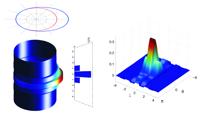
Figure 1: Plot of the Wigner function for a coherent state with $\ell_{0}=0$ and $\phi_{0}=0$. The cylinder extends vertically from $\ell=-4$ to $\ell=+4$. The two corresponding marginal distributions are shown. In the right panel we show the unwrapped version of the Wigner function.

In figure 1, the Wigner function for the coherent state $|\ell_{0}=0,\phi_{0}=0\rangle$ is plotted. A pronounced peak at $\phi=0$ for $\ell=0$ and slightly smaller ones for $\ell=\pm 1$ can be observed. The associated marginal distributions are also plotted. They are strictly positive, as correspond to true probability distributions. For quantitative comparisons, however, sometimes it may be convenient to “cut” this cylindrical plot along a line $\phi$=constant and unwrap it. This is also shown in figure 1.

A closer look at this figure reveals also a remarkable fact: for values close to $\phi=\pm\pi$ and $\ell=\pm 1$, the Wigner function takes negative values. Actually, a numeric analysis suggests the existence of negativities close to $\phi=\pm\pi$ for any odd value of $\ell$.

As our last example, we address the superposition

$$|\Psi\rangle=\frac{1}{\sqrt{2}}(|\ell_{1}\rangle+e^{i\phi_{0}}|\ell_{2}\rangle)$$ (71)

of two angular-momentum eigenstates with a relative phase $e^{i\phi_{0}}$. The Wigner function splits again; now the “even” part reads as

$$W_{|\Psi\rangle}^{(+)}(\ell,\phi)=\frac{1}{4\pi}\{\delta_{\ell,\ell_{1}}+\delta_{\ell,\ell_{2}}+2\delta_{\ell_{1}+\ell_{2},2\ell}\,\cos[\phi_{0}+(\ell_{2}-\ell_{1})\phi]\}\,.$$ (72)

For the “odd” part, the diagonal contributions vanish, and one has

$$W_{|\Psi\rangle}^{(-)}(\ell,\phi)=\frac{1}{\pi^{2}}\cos[\phi_{0}+(\ell_{2}-\ell_{1})\phi]\,\frac{(-1)^{\ell+(\ell_{1}+\ell_{2}-1)/2}}{\ell_{1}+\ell_{2}-2\ell}\delta_{\ell_{1}+\ell_{2}=\mathrm{odd}}\,,$$ (73)

where $\delta_{\ell_{1}+\ell_{2}=\mathrm{odd}}$ indicates that the sum is nonzero only when $\ell_{1}+\ell_{2}$ is odd.

In consequence, when $|\ell_{1}-\ell_{2}|$ is odd, the interference term contains contributions for any $\ell$, damped as $1/\ell$. When $|\ell_{1}-\ell_{2}|$ is an even number, the contribution (73) vanishes and we have three contributions: two flat slices coming from the states $|\ell_{1}\rangle$ and $|\ell_{2}\rangle$ and an interference term located at $\ell=(\ell_{1}+\ell_{2})/2$.

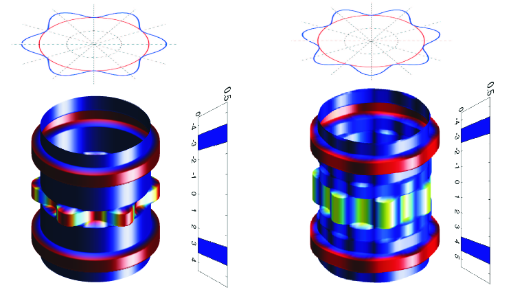
Figure 2: Plot and marginal distributions of the Wigner function for an even superposition $|\ell_{1}\rangle+e^{i\theta}|\ell_{2}\rangle$ with $\ell_{1,2}=\pm 3$ for $\ell=-4$ to $\ell=+4$ (left) and $\ell_{1}=4,\ell_{2}=-3$ for $\ell=-4$ to $\ell=+5$.

These features are nicely illustrated in figure 2. The state $|\Psi\rangle$ is plotted for $\ell_{2}=-3$ and $\ell_{1}=3$ and and $\ell_{2}=-3$ and $\ell_{1}=4$. Changing the relative phase $\phi_{0}$ results in a global rotation of the cylinder. In can be observed in that the two rings at $\ell=-3$ and $\ell=4$ (as opposed to the rings at $\ell=\pm 3$), are not flat in $\phi$, but show a weak dependence on the angle due to the odd contributions added to the flat Kronecker deltas.

In view of these results, one can wonder what are the pure state for which the Wigner function is nonnegative. The answer was found quite recently [78]: the Wigner function $W_{|\Psi\rangle}(\ell,\phi)$ is nonnegative if and only if $|\Psi\rangle$ is an angular momentum eigenstate $|\ell_{0}\rangle$. The proof is rather technical and we skip it. The important point we wish to stress is that while for the continuous case the notions of coherent states, Gaussian wave packets, and states with nonnegative Wigner functions are completely equivalent, special care must be paid in extending these ideas to other physical systems, like angle-angular momentum, since they lose their equivalence.

To round up this section, we illustrate the benefits of our phase-space approach by dealing with the evolution of the “quantum” pendulum

$$\hat{H}=\frac{\hat{L}^{2}}{2}+\frac{\lambda}{2}\left(\hat{E}+\hat{E}^{\dagger}\right)\,.$$ (74)

which has been proposed as a good candidate to describe the evolution of the wave function of Josephson junctions [79]. The corresponding Weyl symbol is

$$h(\ell,\phi)=\frac{1}{2\pi}\left(\frac{\ell^{2}}{2}+\lambda\cos\phi\right)\,.$$ (75)

Using the relations (66), we get the evolution equation for the Wigner function

$$\frac{\partial}{\partial t}W(\ell,\phi)=-\frac{1}{2\pi}\left[\frac{\ell}{2}\frac{\partial}{\partial\phi}-2\lambda\sin\phi\sinh(\delta_{\ell}/2)\right]W(\ell,\phi)\,.$$ (76)

We can directly check that $\exp(\delta_{ell}/2)W(\ell,\phi)=W(\ell+1/2,\phi)$, so (76) becomes

$$\frac{\partial}{\partial t}W(\ell,\phi)=-\frac{1}{2\pi}\left(\frac{\ell}{2}\frac{\partial}{\partial\phi}W(\ell,\phi)-\lambda\sin\phi[W(\ell+1/2,\phi)-W(\ell-1/2,\phi)]\right)\,.$$ (77)

We are interested in the semiclassical evolution, i.e., for states whose angular momentum components are sufficiently concentrated around a certain value $\ell_{0}$ with $|\ell_{0}|\gg 1$. Thus, we may view $W(\ell+1/2,\phi)-W(\ell-1/2,\phi)$ as a derivative respect to $\ell$, so we finally get

$$\frac{\partial}{\partial t}W(\ell,\phi)=-\frac{1}{2\pi}\left(\frac{\ell}{2}\frac{\partial}{\partial\phi}-\lambda\sin\phi\frac{\partial}{\partial\ell}\right)W(\ell,\phi)\,,$$ (78)

whose formal solution is $W(\ell(t),\phi(t))$ in terms of the “classical” trajectories

$$\dot{\ell}=-2\lambda\sin\phi,\qquad\dot{\phi}=-\ell.$$ (79)

This constitutes a nice solution for an involved problem.

4.1 Tomography

To complete our theory we propose a reconstruction scheme for observables in this cylindrical phase space. The equivalent version of (37) reads now, particularized for the density operator,

$$\hat{\varrho}=\sum_{{\ell}\in\mathbb{Z}}\int_{-\pi}^{\pi}\varrho(\ell,\phi)\,\hat{D}(\ell,\phi)\,d\phi\,,$$ (80)

where $\varrho(\ell,\phi)=\mathop{\mathrm{Tr}}\nolimits[\hat{\varrho}\,\hat{D}^{\dagger}(\ell,\phi)]/(2\pi)$. In terms of $\varrho(\ell,\phi)$, the Wigner function is

$$W_{\hat{\varrho}}(\ell,\phi)=\frac{1}{2\pi}\sum_{{\ell^{\prime}}\in\mathbb{Z}}\int_{-\pi}^{\pi}\exp[i(\ell^{\prime}\phi-\ell\phi^{\prime})]\,\varrho(\ell^{\prime},\phi^{\prime})\,d\phi^{\prime}\,.$$ (81)

A reconstruction of this Wigner function is thus tantamount to finding the coefficients $\varrho(\ell,\phi)$. For $\ell=0$, these coefficients

$$\varrho(0,\phi)=\frac{1}{2\pi}\sum_{{\ell}\in\mathbb{Z}}\exp(i\ell\phi)\,\langle\ell|\hat{\varrho}|\ell\rangle$$ (82)

are simply the Fourier transform of the angular-momentum spectrum.

For $\ell\neq 0$, we assume that we are able to experimentally determine $\hat{L}^{2}$ transformations on the input state followed by angular projections, that is,

$$p(\phi,\zeta)=\langle\phi|\exp(i\zeta\hat{L}^{2}/2)\,\hat{\varrho}\,\exp(-i\zeta\hat{L}^{2}|\phi\rangle\,.$$ (83)

One can check that

$$\varrho(\ell,\phi)=\frac{1}{2\pi}\int_{-\pi}^{\pi}\exp(-i\ell\phi^{\prime})\,p(\phi^{\prime},\phi/\ell)\,d\phi^{\prime}\,,$$ (84)

so the measurement of $p(\phi,\zeta)$ allows for the determination $\varrho(\ell,\phi)$ and hence the full reconstruction of the Wigner function via equation (81).

As a rather simple yet illustrative example, let us note that for the vortex state $|\ell_{0}\rangle$, $\hat{L}^{2}$ is diagonal, so the tomograms $p(\phi^{\prime},\phi^{\prime}/\ell)$ are independent of $\phi$ and $\ell$ and all of them equal to $1/(2\pi)$. Performing the integration we obtain precisely the Wigner function in equation (67).

The feasibility of the proposed scheme relies on two crucial points. First, the implementation of the $\hat{L}^{2}$ transformation, which corresponds to a free rotor. This has been used to describe the evolution in a variety of situations. Second, we need to assess the measurement of the angular spectrum, which can be done only approximately. Though the implementation of this scheme may differ depending on the system under considerations, our formulation provides a common theoretical framework on the Hilbert space generated by the action of angle and angular momentum. A experimental demonstration of the method in terms of optical beams has been recently established [80].

For continuous variables, it is possible to make a direct sampling of the Wigner function by a scheme that determines the parity [81, 82]. This is an unexplored territory for the cylinder that is worth investigating.

5 Concluding remarks

In summary, we have shown how to extend in a consistent way all the techniques developed for a continuous-variable phase space to the case of angle and angular momentum. While we have not left aside the mathematical details, our main emphasis has been on presenting a simple and useful toolkit that any practitioner in the field should master. In our view, far from being an academic curiosity, the ideas expressed here have a wide range of potential applications in numerous hot topics.

This paper has greatly benefited from the criticism and advice of Prof. B.-G. Englert. The work was supported by the Spanish Research Directorate (Grants FIS2005-06714 and FIS2008-04356), the UCM-BCSH program (Grant GR-920992), the Mexican CONACyT (Grant 106525), the Czech Ministry of Education (Project MSM6198959213), and the Czech Ministry of Industry and Trade (Project FR-TI1/364).

References

- Weyl [1928] H. Weyl, Gruppentheorie und Quantemechanik, Hirzel-Verlag, Leipzig, 1928.
- Wigner [1932] E. P. Wigner, Phys. Rev. 40 (1932) 749–759.
- Moyal [1949] J. E. Moyal, Proc. Cambridge Phil. Soc. 45 (1949) 99–124.
- Stratonovich [1956] R. L. Stratonovich, JETP 31 (1956) 1012—1020.
- Agarwal and Wolf [1970] G. S. Agarwal, E. Wolf, Phys. Rev. D 2 (1970) 2161–2186.
- Berezin [1975] F. A. Berezin, Commun. Math. Phys. 40 (1975) 153–174.
- Agarwal [1981] G. S. Agarwal, Phys. Rev. A 24 (1981) 2889–2896.
- Bertrand and Bertrand [1987] J. Bertrand, P. Bertrand, Found. Phys. 17 (1987) 397–405.
- Varilly and Gracia-Bondía [1989] J. C. Varilly, J. M. Gracia-Bondía, Ann. Phys. 190 (1989) 107–148.
- Brif and Mann [1998] C. Brif, A. Mann, J. Phys. A 31 (1998) L9–L17.
- Benedict and Czirják [1999] M. G. Benedict, A. Czirják, Phys. Rev. A 60 (1999) 4034–4044.
- Tatarskii [1983] V. I. Tatarskii, Sov. Phys. Usp. 26 (1983) 311–327.
- Balazs and Jennings [1984] N. L. Balazs, B. K. Jennings, Phys. Rep. 104 (1984) 347–391.
- Hillery et al. [1984] M. Hillery, R. F. O. Connell, M. O. Scully, E. P. Wigner, Phys. Rep. 106 (1984) 121–167.
- Lee [1995] H.-W. Lee, Phys. Rep. 259 (1995) 147–211.
- Schroek [1996] F. E. Schroek, Quantum Mechanics on Phase Space, Kluwer, Dordrecht, 1996.
- Schleich [2001] W. P. Schleich, Quantum Optics in Phase Space, Wiley-VCH, Berlin, 2001.
- Zachos et al. [2005] C. K. Zachos, D. B. Fairlie, T. L. Curtright (Eds.), Quantum Mechanics in Phase Space, World Scientific, Singapore, 2005.
- Wootters [1987] W. K. Wootters, Ann. Phys. 176 (1987) 1–21.
- Galetti and de Toledo-Piza [1988] D. Galetti, A. F. R. de Toledo-Piza, Physica A 149 (1988) 267–282.
- Galetti and de Toledo-Piza [1992] D. Galetti, A. F. R. de Toledo-Piza, Physica A 186 (1992) 513–523.
- Wootters [2004] W. K. Wootters, IBM J. Res. Dev. 48 (2004) 99–110.
- Gibbons et al. [2004] K. S. Gibbons, M. J. Hoffman, W. K. Wootters, Phys. Rev. A 70 (2004) 062101.
- Vourdas [2004] A. Vourdas, Rep. Prog. Phys. 67 (2004) 267–320.
- Klimov et al. [2006] A. B. Klimov, C. Muñoz, J. L. Romero, J. Phys. A 39 (2006) 14471–14497.
- Vourdas [2007] A. Vourdas, J. Phys. A 40 (2007) R285–R331.
- Björk et al. [2008] G. Björk, A. B. Klimov, L. L. Sánchez-Soto, Prog. Opt. 51 (2008) 469–516.
- Klimov et al. [2009] A. B. Klimov, J. L. Romero, G. Björk, L. L. Sánchez-Soto, Ann. Phys. 324 (2009) 53–72.
- Durt et al. [2010] T. Durt, B.-G. Englert, I. Bengtsson, K. Zyczkowski, Int. J. Quantum Inf. 8 (2010) 535–640.
- Laidlaw and DeWitt [1971] M. G. G. Laidlaw, C. M. DeWitt, Phys. Rev. D 3 (1971) 1375–1378.
- Schulman [1971] L. S. Schulman, J. Math. Phys. 12 (1971) 304–308.
- Dowker [1972] J. S. Dowker, J. Phys. A 5 (1972) 936–943.
- Acerbi et al. [1993] F. Acerbi, G. Morchio, F. Strocchi, Lett. Math. Phys. 27 (1993) 1–11.
- Allen et al. [2003] L. Allen, S. M. Barnett, M. J. Padgett, Optical Angular Momentum, Institute of Physics Publishing, Bristol, 2003.
- Andrews [2008] D. L. Andrews (Ed.), Structured Light and Its Applications, Academic Press, Boston, 2008.
- Molina-Terriza et al. [2007] G. Molina-Terriza, J. P. Torres, L. Torner, Nat. Phys. 3 (2007) 305–310.
- Franke-Arnold et al. [2008] S. Franke-Arnold, L. Allen, M. Padgett, Laser Photon. Rev. 2 (2008) 299–313.
- Vaziri et al. [2002] A. Vaziri, G. Weihs, A. Zeilinger, J. Opt. B 4 (2002) S47–S51.
- Langford et al. [2004] N. K. Langford, R. B. Dalton, M. D. Harvey, J. L. O’Brien, G. J. Pryde, A. Gilchrist, S. D. Bartlett, A. G. White, Phys. Rev. Lett. 93 (2004) 053601.
- Carruthers and Nieto [1968] P. Carruthers, M. M. Nieto, Rev. Mod. Phys. 40 (1968) 411–440.
- Lynch [1995] R. Lynch, Phys. Rep. 256 (1995) 367–436.
- Peřinova et al. [1998] V. Peřinova, A. Lukš, J. Peřina, Phase in Optics, World Scientific, Singapore, 1998.
- Luis and Sánchez-Soto [2000] A. Luis, L. L. Sánchez-Soto, Prog. Opt. 44 (2000) 421–481.
- Mukunda [1979] N. Mukunda, Am. J. Phys. 47 (1979) 182–187.
- Mukunda et al. [2005] N. Mukunda, G. Marmo, A. Zampini, S. Chaturvedi, R. Simon, J. Math. Phys. 46 (2005) 012106.
- Bizarro [1994] J. P. Bizarro, Phys. Rev. A 49 (1994) 3255–3276.
- Vourdas [1996] A. Vourdas, J. Phys. A 29 (1996) 4275–4288.
- Nieto et al. [1998] L. M. Nieto, N. M. Atakishiyev, S. M. Chumakov, K. B. Wolf, J. Phys. A 31 (1998) 3875—3895.
- Ruzzi and Galetti [2002] M. Ruzzi, D. Galetti, J. Phys. A 35 (2002) 4633–4640.
- Zhang and Vourdas [2003] S. Zhang, A. Vourdas, J. Math. Phys. 44 (2003) 5084–5094.
- Kakazu and Sakai [2006] K. Kakazu, E. Sakai, Prog. Theor. Phys. 115 (2006) 1027–1045.
- Kowalski et al. [1996] K. Kowalski, J. Rembieliński, L. C. Papaloucas, J. Phys. A 29 (1996) 4149–4167.
- González and del Olmo [1998] J. A. González, M. A. del Olmo, J. Phys. A 31 (1998) 8841–8857.
- Ohnuki and Kitakado [1993] Y. Ohnuki, S. Kitakado, J. Math. Phys. 34 (1993) 2827–2851.
- Hall and Mitchell [2002] B. C. Hall, J. J. Mitchell, J. Math. Phys. 43 (2002) 1211–1236.
- Ruzzi et al. [2006] M. Ruzzi, M. A. Marchiolli, E. C. da Silva, D. Galetti, J. Phys. A 39 (2006) 9881–9890.
- Rigas et al. [2010] I. Rigas, L. L. Sánchez-Soto, A. B. Klimov, J. Řeháček, Z. Hradil, Opt. Spectrosc. 108 (2010) 206–212.
- Kastrup [2006] H. A. Kastrup, Phys. Rev. A 73 (2006) 052104.
- Rigas et al. [2008] I. Rigas, L. L. Sánchez-Soto, A. B. Klimov, J. Řeháček, Z. Hradil, Phys. Rev. A 78 (2008) 060101.
- Binz and Pods [2008] E. Binz, S. Pods, The Geometry of Heisenberg Groups, American Mathematical Society, Providence, 2008.
- Galindo and Pascual [1991] A. Galindo, P. Pascual, Quantum Mechanics, Springer, Berlin, 1991.
- Kenfack and Życzkowski [2004] A. Kenfack, K. Życzkowski, J. Opt. B 6 (2004) 396–404.
- Hudson [1974] R. L. Hudson, Rep. Math. Phys. 6 (1974) 249–252.
- Janssen [1984] A. J. E. M. Janssen, SIAM J. Math. Anal. 15 (1984) 170–176.
- Lieb [1990] E. H. Lieb, J. Math. Phys. 31 (1990) 594–599.
- Perelomov [1986] A. Perelomov, Generalized Coherent States and their Applications, Springer, Berlin, 1986.
- Mehta [1987] M. L. Mehta, J. Math. Phys. 28 (1987) 781–785.
- Ruzzi [2006] M. Ruzzi, J. Math. Phys. 47 (2006) 063507.
- Paris and Řeháček [2004] M. G. A. Paris, J. Řeháček (Eds.), Quantum State Estimation, volume 649 of Lect. Not. Phys., Springer, Heidelberg, 2004.
- Lvovsky and Raymer [2009] A. I. Lvovsky, M. G. Raymer, Rev. Mod. Phys. 81 (2009) 299–332.
- Emch [1972] G. G. Emch, Algebraic Methods in Statistical Mechanics and Quantum Field Theory, Wiley, New York, 1972.
- Uffink [1990] J. B. M. Uffink, Measures of Uncertainty and the Uncertainty Principle, Ph.D. thesis, University of Utrecht, 1990.
- Bracewell [1999] R. Bracewell, The Fourier Transform and Its Applications, McGraw-Hill, 3rd ed edition, 1999.
- Hradil et al. [2006] Z. Hradil, J. Řeháček, Z. Bouchal, R. Čelechovský, L. L. Sánchez-Soto, Phys. Rev. Lett. 97 (2006) 243601.
- Řeháček et al. [2008] J. Řeháček, Z. Bouchal, R. Čelechovský, Z. Hradil, L. L. Sánchez-Soto, Phys. Rev. A 77 (2008) 032110.
- Plebański et al. [2000] J. F. Plebański, M. Prazanowski, J. Tosiek, F. K. Turrubiates, Acta Phys. Pol. B 31 (2000) 561–587.
- Mumford [1983] D. Mumford, Tata Lectures on Theta I, Birkhauser, Boston, 1983.
- Rigas et al. [2009] I. Rigas, L. L. Sánchez-Soto, A. B. Klimov, J. Řeháček, Z. Hradil, Phys. Rev. A (2009).
- Anglin et al. [2001] J. R. Anglin, P. Drummond, A. Smerzi, Phys. Rev. A 64 (2001) 063605.
- Řeháček et al. [2010] J. Řeháček, Z. Hradil, Z. Bouchal, A. B. Klimov, I. Rigas, L. L. Sánchez-Soto, Opt. Lett. 35 (2010) 2064–2066.
- Englert et al. [1993] B.-G. Englert, N. Sterpi, H. Walther, Opt. Commun. 100 (1993) 526–535.
- Bertet et al. [2002] P. Bertet, A. Auffeves, P. Maioli, S. Osnaghi, T. Meunier, M. Brune, J. M. Raimond, S. Haroche, Physical Review Letters 89 (2002) 200402.