H i Observations of the Asymptotic Giant Branch Star X Herculis: Discovery of an Extended Circumstellar Wake Superposed on a Compact High-Velocity Cloud

Abstract

We report H i 21-cm line observations of the asymptotic giant branch (AGB) star X Her obtained with the Robert C. Byrd Green Bank Telescope (GBT) and the Very Large Array (VLA). We have unambiguously detected H i emission associated with the circumstellar envelope of the star, with a mass totaling $M_{\rm HI}\approx 2.1\times 10^{-3}~{}M_{\odot}$. The H i distribution exhibits a head-tail morphology, similar to those previously observed around the AGB stars Mira and RS Cnc. The tail is elongated along the direction of the star’s space motion, with a total extent of  $>$$\sim$$6^{\prime}\,.0$ (0.24 pc) in the plane of the sky. We also detect a systematic radial velocity gradient of $\sim$6.5 km s^-1 across the H i envelope. These results are consistent with the H i emission tracing a turbulent wake that arises from the motion of a mass-losing star through the interstellar medium (ISM). GBT mapping of a $2^{\circ}\times 2^{\circ}$ region around X Her reveals that the star lies (in projection) near the periphery of a much larger H i cloud that also exhibits signatures of interaction with the ISM. The properties of the cloud are consistent with those of compact high-velocity clouds. Using ¹²CO $J$=1-0 observations, we have placed an upper limit on its molecular gas content of $N_{H2}<1.3\times 10^{20}$ cm^-2. Although the distance to the cloud is poorly constrained, the probability of a chance coincidence in position, velocity, and apparent position angle of space motion between X Her and the cloud is extremely small, suggesting a possible physical association. However, the large H i mass of the cloud ($~{}\hbox to0.0pt{$>$\hss}{\lower 4.30554pt\hbox{$\sim$}}2.4~{}M_{\odot}$) and the blueshift of its mean velocity relative to X Her are inconsistent with an origin tied directly to ejection from the star.

1 Introduction

Stars on the asymptotic giant branch (AGB) undergo copious mass-loss through cool, low-velocity winds ($V_{\rm outflow}\sim$10 km s^-1). The material dispersed by these winds supplies a primary source of chemical enrichment to the interstellar medium (ISM; e.g., Cristallo et al. 2009 and references therein). In addition, the outflows and space motions of these mass-losing stars play a role in shaping the structure of the ISM on parsec and sub-parsec scales (Villaver et al. 2003; Wareing et al. 2007b). Furthermore, the distribution of circumstellar debris on the largest scales may be important for the evolution of planetary nebulae as well as some Type Ia supernovae (e.g., Wang et al. 2004; Deng et al. 2004).

It has long been recognized that the interstellar environment of evolved stars can have a profound impact on the ultimate mass, size, shape, and chemical composition of their circumstellar envelopes (hereafter CSEs; e.g., Smith 1976; Isaacman 1979; Serabyn et al. 1991; Young et al. 1993; Zijlstra & Weinberger 2002; Villaver et al. 2002, 2003; Wareing et al. 2006b; 2007a, b, c; see also the review by Stencel 2009). Nonetheless, this has been largely ignored in many theoretical investigations of AGB star evolution, which still treat such stars as evolving in isolation. Moreover, the interfaces through which AGB stars interact with their environments have remained poorly studied observationally. One problem is that CSEs can be enormously extended ( $>$$\sim$1 pc), and their chemical composition changes as a function of distance from the star, as densities drop and molecules become dissociated by the interstellar radiation field or other radiation sources. The result is that the some of the most frequently used observational tracers of CSEs (e.g., CO; SiO, H₂O, and OH masers) do not probe the outermost CSE or its interaction zone with the ISM. In some cases, more extended material can be traced via imaging observations in the infrared (Zijlstra & Weinberger 2002; Ueta et al. 2006, 2010a, b; Ladjal et al. 2010) or in the far-ultraviolet (Martin et al. 2007; Sahai & Chronopoulos 2010), but such data do not supply any direct kinematic information.

Our recent work has demonstrated that the H i 21-cm line of neutral hydrogen is a powerful tool for the study of extended CSEs and their interface with their larger-scale environments (e.g., Gérard & Le Bertre 2006; Matthews & Reid 2007; Libert et al. 2007, 2008, 2010a,b; Matthews et al. 2008). Not only is hydrogen the most plentiful constituent of CSEs, but H i line measurements provide kinematic information and can be directly translated into H i mass measurements. Furthermore, because H i is not destroyed by the interstellar radiation field, H i measurements are particularly well-suited to probing the outermost reaches of CSEs.

In this paper, we continue our investigation of the H i properties of evolved stars with a study of the nearby, semi-regular variable star X Herculis (X Her). For the first time, we combine Very Large Array (VLA) H i imaging observations with H i mapping obtained with the Robert C. Byrd Green Bank Telescope (GBT). In concert, these observations allow us to probe the CSE and its environs on spatial scales ranging from $\sim 1^{\prime}$ to $\sim 1^{\circ}$. At the smaller scales, our observations complement previous studies of the inner CSE from CO and SiO line observations. On large scales, our observations show that X Her overlaps in velocity and projected position with a compact high velocity cloud. We investigate the properties of this cloud in detail and evaluate the possibility that it could be associated with X Her.

2 An Overview of X Her

2.1 Stellar Properties

X Her is an oxygen-rich, semi-regular variable star of type SRb and a spectral classification that ranges in the literature from M6 to M8. Its rather large velocity relative to the local standard of rest ($V_{\rm LSR}\approx-73$ km s^-1; Knapp et al. 1998) makes it well-suited for H i observations, since it is well-separated from the bulk of the Galactic emission along the line-of-sight. The star has been found to have both short and long pulsation cycles; periods of 102 and 178 days have been reported by Kiss et al. (1999) based on photometric measurements, while Hinkle et al. (2002) found a longer period of 658 days based on a spectroscopic analysis. The mass and luminosity of X Her are estimated to be $1.9~{}M_{\odot}$ and 3570 $L_{\odot}$, respectively (Dyck et al. 1998; Dumm & Schild 1998). Some additional stellar properties of X Her are summarized in Tables 1 & 2. Throughout this work we adopt a distance of $d_{*}\approx$140 pc based on the Hipparcos parallax measurement of 7.30$\pm$0.40 mas (van Leeuwen 2007).

Table 1: Coordinates and Stellar Properties of X Herculis

Parameter	Value	Ref.
$\alpha$ (J2000.0)	16 02 39.2	1
$\delta$ (J2000.0)	+47 14 25.3	1
$l$	$74^{\circ}\,.46$	1
$b$	$+47^{\circ}\,.78$	1
Distance	140 pc	2
Chemistry	Oxygen-rich	3
Variable Class	SRb	3
Spectral Type	M6-M8	1,4
Periods	102$\pm$5, 178$\pm$5 days, 658.3$\pm$17.0 days	4,5
$T_{\rm eff}$	3281$\pm$130 K	6
Radius	183$\pm$4 $R_{\odot}$	6
Luminosity	3570 $L_{\odot}$	6
Mass	1.9 $M_{\odot}$	7
${\dot{M}}$	(0.34,1.1)$\times 10^{-7}~{}M_{\odot}$ yr-1	8
$V_{\rm outflow}$	3.5 & 9 km s-1	8

Note. — Units of right ascension are hours, minutes, and seconds, and units of declination are degrees, arcminutes, and arcseconds. All quantities have been scaled to the distance adopted in this paper.

References. — (1) SIMBAD database; (2) van Leeuwen 2007; (3) Loup et al. 1993; (4) Hinkle et al. 2002; (5) Kiss et al. 1999. (6) Dyck et al. 1998; (7) Dumm & Schild 1998; (8) Knapp et al. 1998.

Table 2: Previous Radial Velocity Measurements and Mass-Loss Estimates for X Her

Line	$V_{\rm LSR}$ (km s-1)	$V_{\rm out}$ (km s-1)	${\dot{M}}$ ($M_{\odot}$ yr-1)	Ref.
K i	$-80$	…	…	1
Infrared	$-72.8$	…	…	2
SiO(2-1)	$-72.0$	2.5	$4.0\times 10^{-8}$	3
SiO(2-1)	$-73.0$	6.5	$1.5\times 10^{-7}$	3
SiO(5-4)	…	4.9	…	4
CO(1-0)	$-71.0$	6.5	$1.5\times 10^{-7}$	5
CO(2-1)	$-73.2\pm 0.4$	3.2$\pm 0.5$	$3.4\times 10^{-8}$	6
CO(2-1)	$-72.8\pm 0.8$	8.5$\pm$1.0	$1.1\times 10^{-7}$	6
CO(3-2)	$-73.1\pm 0.3$	3.5$\pm 1.4$	$3.4\times 10^{-8}$	6
CO(3-2)	$-73.2\pm 0.5$	9.0$\pm 1.0$	$1.1\times 10^{-7}$	6
H i	$-70.6$	2	$\sim 10^{-7}$	7
H i	$-72.2$	6.5	$\sim 10^{-7}$	7

Note. — Explanation of columns: (1) spectral line used for the measurement; (2) radial velocity relative to the local standard of rest (LSR); (3) outflow velocity; (4) derived mass-loss rate in solar masses per year; (5) reference. Two sets of parameters are quoted for a given spectral line in cases where the line profile was found to be complex.

References. — (1) Wallerstein & Dominy 1988; (2) Hinkle et al. 2002; (3) González Delgado et al. 2003; (4) Sahai & Wannier 1992; (5) Kerschbaum et al. 1996; (6) Knapp et al. 1998; (7) Gardan et al. 2006.

2.2 Previous Studies of the X Her CSE

One of the first detailed studies of the CSE of X Her was by Kahane & Jura (1996), who used the IRAM 30-m telescope to map the circumstellar CO(1-0) and CO(2-1) emission. The authors found the CO line profile shapes to be more complex than those seen in many other AGB stars, comprising both broad and narrow components whose spectral widths correspond to outflow velocities of $\sim$10 km s^-1 and $\sim$3 km s^-1, respectively (see also Knapp et al. 1998). Kahane & Jura were also able to marginally resolve the CSE spatially in their CO(2-1) observations (with a beam FWHM of $12^{\prime\prime}$); based on these data, they argued for the existence of a multi-component wind, including a weakly collimated bipolar outflow.

Subsequent higher resolution CO(1-0) imaging observations by Nakashima (2005; FWHM$\approx 3^{\prime\prime}$) confirmed the presence of a bipolar outflow associated with the broader line component of X Her. This outflow extends to $\sim\pm 10^{\prime\prime}$ ($\pm$1400 AU) from the star. Nakashima suggested that the narrower CO line component might arise either from a second, smaller-scale bipolar outflow, or from a disk that is rotating or expanding. More recent CO imaging observations by Castro-Carrizo et al. (2010) with 1^′′-2^′′ resolution support the latter interpretation—i.e., an expanding, equatorial disk that lies perpendicular to the larger-scale bipolar flow.

The presence of these pronounced deviations from spherical symmetry already during the AGB phase suggests the possibility that X Her may be a binary (Kahane & Jura 1996). However, to date, both speckle interferometry (Lu et al. 1987) and radial velocity searches have failed to provide any evidence for a companion. Radial velocity variations are present, but appear to be due to the star’s pulsation (Hinkle et al. 2002).

In 2006, Gardan et al. published the first H i 21-cm line detection of X Her based on observations with the Nançay Radio Telescope (NRT). The H i line profile obtained by these authors appeared to be composite, comprising both broad (FWHM$\sim$13 km s^-1) and narrow (FWHM$\sim$4 km s^-1) components. However, the linewidths and velocity centroids of these components differed from the broad and narrow line components seen in CO and SiO (Table 2), suggesting they were not obviously related. Based on NRT mapping, Gardan et al. found evidence that the broad H i component arose from material extending over $~{}\hbox to0.0pt{$>$\hss}{\lower 4.30554pt\hbox{$\sim$}}10^{\prime}$ and that was asymmetrically distributed about the star, with a concentration to the northeast. Meanwhile, the narrow component appeared to be unresolved ($<4^{\prime}$) and centered on the star. The total mass of circumstellar hydrogen inferred from the NRT study was $M_{\rm HI}\approx 6.5\times 10^{-3}~{}M_{\odot}$.

Gardan et al. (2006) suggested that the broad H i line component that they observed might be explained by asymmetric mass loss, with an outflow along a preferred direction. The implications of this would be significant, since it would indicate the existence of pronounced large-scale asymmetries in the circumstellar ejecta during the AGB stage—in stark contrast to the commonly held picture of spherical mass-loss (cf. Huggins et al. 2009). Further, this would suggest that the circumstellar atomic hydrogen is largely decoupled from the axisymmetric morphology of the CSE traced on smaller scales via CO emission.

Unfortunately, the limited resolution of the NRT beam [$4^{\prime}$ (E-W)$\times 22^{\prime}$ (N-S)] permits only a coarse characterization of the distribution of H i emission around X Her and its relationship to structures in the CSE on smaller scales. Furthermore, the need to decompose the circumstellar signal from contaminating interstellar emission introduces uncertainties in the line decomposition and derived H i fluxes. For these reasons, we have obtained new, higher spatial resolution H i observations of X Her and its environs using a combination of the VLA and the GBT. In this paper, we describe our new and improved characterization of the large-scale properties of the X Her’s CSE that have resulted from these observations. In addition, we investigate a new puzzle uncovered by our observations—namely the relationship between the CSE of X Her and an adjacent “high-velocity” H i cloud.

3 VLA Observations

X Her was observed in the H i 21-cm line with the VLA of the National Radio Astronomy Observatory (NRAO) on 2007 May 5 and 2007 May 10 using the most compact (D) configuration (0.035-1.0 km baselines). This provided sensitivity to emission on scales of up to $\sim$15^′. The primary beam of the VLA at our observing frequency of 1420.3 MHz is $\sim 31^{\prime}$.

The VLA correlator was used in dual polarization (2AC) mode with a 0.78 MHz bandpass, yielding 256 spectral channels with 3.05 kHz ($\sim$0.64 km s^-1) spacing. The band was centered at a velocity of $-100$ km s^-1 relative to the local standard of rest (LSR); the band center was offset slightly from the systemic velocity of the star ($V_{\rm sys,LSR}\approx-73$ km s^-1; see Table 2) to shift strong Galactic emission away from the band edge.

Observations of X Her were interspersed with observations of the phase calibrator, 1625+415, approximately every 20 minutes. 3C286 (1331+305) was used as a flux calibrator, and an additional strong point source (1411+522) was observed as a bandpass calibrator. To insure that the absolute flux scale and bandpass calibration were not corrupted by Galactic emission in the band, the flux and bandpass calibrators were each observed twice, first with the band shifted by $+$1 MHz and then by $-1$ MHz, relative to the band center used for the observations of X Her and 1625+415. 1625+415 was also observed once at each of these offset frequencies to allow more accurate bootstrapping of the absolute flux scale to the X Her data. The resulting flux scale has an uncertainty of $\sim$5% (see below). In total, $\sim$6.8 hours of integration were obtained on X Her. Approximately 6% of the observed visibilities were flagged because of radio frequency interference (RFI) or hardware problems.

The VLA data were calibrated and reduced using the Astronomical Image Processing System (AIPS). At the time of our observations, the VLA contained 26 operating antennas, 9 of which had been retrofitted as part of the Expanded Very Large Array (EVLA) upgrade. The use of this “hybrid” array necessitated special care in the data reduction process.

Traditionally, the calibration of VLA data sets make use of a “channel 0” data set formed by taking a vector average of the inner 75% of the observing band. However, the mismatch in bandpass response between the VLA and EVLA antennas causes closure errors in the default channel 0 computed this way. Furthermore, the hardware used to convert the digital signals from the EVLA antennas into analog signals for the VLA correlator causes aliased power in the bottom 0.5 MHz of the baseband (i.e., at low-numbered channels). This aliasing is of consequence because of the narrow bandwidth used for our observations. However, it affects EVLA-EVLA baselines only, as it does not correlate on ELVA-VLA baselines.

To mitigate the above effects, we used the following modified approach to the gain calibration. We first applied hanning smoothing to the visibility data and discarded every other channel, resulting in a 128-channel data set. After applying the latest available corrections to the antenna positions and an initial excision of corrupted data, we computed and applied an initial bandpass calibration to our spectral line data to remove closure errors on VLA-EVLA baselines. EVLA-EVLA baselines were flagged during this step. We then computed a new frequency-averaged (channel 0) data set for use in calibrating the frequency-independent complex gains. We excluded from this average the bottom $\sim$0.5 MHz portion of band affected by aliasing (channels 1-79) as well as several edge channels on the upper portion of the band (channels 121-128). After solving for the frequency-independent portion of the complex gains using the newly computed channel 0 file, we computed and applied an additional correction to the bandpass, and then applied time-dependent frequency shifts to the data to compensate for changes caused by the Earth’s motion during the course of the observations.

Prior to imaging the line data, the $u$-$v$ data were continuum-subtracted using a linear fit to the real and imaginary components of the visibilities. Channels 21-32 and 59-120 were determined to be line-free and were used for these fits. These channel ranges correspond to LSR velocities of $-44.6$ to $-58.8$ km s^-1 and $-93.6$ to $-172.1$ km s^-1, respectively. Although the spectral shape of the aliased portion of the continuum as measured toward our continuum calibrators was better approximated by a fourth order polynomial, there was insufficient continuum signal in our line data to adequately constrain such high order fits.

We imaged the VLA line data using the standard AIPS CLEAN deconvolution algorithm and produced data cubes using various weighting schemes (Table 4). We also produced an image of the 21-cm continuum emission in the X Her field using the line-free portion of the band. The peak continuum flux density within the primary beam was $\sim$0.35 Jy. We compared the measured flux densities of several sources in the field with those from the NRAO VLA Sky Survey (Condon et al. 1998) and found agreement to within $\pm$4%.

We found no evidence for 21-cm continuum emission associated with X Her or its circumstellar envelope. We detected a weak ($\sim$12 mJy), unresolved continuum source offset from the position of X Her by $2^{\prime}\,.4$ and overlapping with the star’s H i emission. However, inspection of the Digitized Sky Survey reveals that this most likely arises from a pair of distant, interacting galaxies that are coincident with this position.

Table 3: VLA Calibration Sources

Source	$\alpha$(J2000.0)	$\delta$(J2000.0)	Flux Density (Jy)	Date
3C286a	13 31 08.2879	+30 32 32.958	14.72∗	2007May 5 & 10
1411+522b	14 11 20.6477	+52 12 09.141	22.27$\pm$0.20∗	2007 May 5
…	…	…	22.07$\pm$0.14∗	2007 May 10
1625+415c	16 25 57.6697	+41 34 40.629	1.50$\pm$0.01	2007 May 5
…	…	…	1.50$\pm$0.01	2007 May 10

Note. — Units of right ascension are hours, minutes, and seconds, and units of declination are degrees, arcminutes, and arcseconds.

Table 4: Deconvolved Image Characteristics

Image	$\cal R$	Taper	$\theta_{\rm FWHM}$	PA	rms
Descriptor		(k$\lambda$,k$\lambda$)	(arcsec)	(degrees)	(mJy beam-1)
(1)	(2)	(3)	(4)	(5)	(6)
Robust +1	+1	…	$53^{\prime\prime}\times 48^{\prime\prime}$	$-37$	0.93-1.10
Natural	+5	…	$59^{\prime\prime}\times 55^{\prime\prime}$	$-42$	0.90-1.07
Tapered	+5	2,2	$112^{\prime\prime}\times 93^{\prime\prime}$	$+47$	1.05-1.33
Continuum	+1	…	$52^{\prime\prime}\times 48^{\prime\prime}$	$-37$	0.26

Note. — Explanation of columns: (1) image or data cube designation used in the text; (2) robustness parameter used in image deconvolution (see Briggs 1995); (3) Gaussian taper applied in $u$ and $v$ directions, expressed as distance to 30% point of Gaussian in units of kilolambda; (4) dimensions of synthesized beam; (5) position angle of synthesized beam (measured east from north); (6) rms noise per channel (1$\sigma$; line data) or in frequency-averaged data (continuum).

4 Green Bank Telescope Observations

To better characterize the extended emission distribution of X Her and its larger-scale environment, we obtained H i mapping observations of the X Her field using the 100-m Robert C. Byrd Green Bank Telescope (GBT) of the NRAO on 2008 February 21, 25, 26, and 27. The GBT spectrometer was employed with a 12.5 MHz bandwidth and 9-level sampling. In the raw data, there were 16,384 spectral channels with a 0.7629 kHz (0.16 km s^-1) channel width. In-band frequency switching was used with cycles of 0.8 Hz, alternating between frequency shifts of 0 and $-2.5$ MHz from the center frequency of 1420.4058 MHz. This resulted in a usable LSR velocity range from $-480$ to $+480$ km s^-1. Data were recorded in dual linear polarizations. System temperatures during the run ranged from 15-18 K. The spectral brightness temperature scale was determined from injection of a noise diode signal at a rate of 0.4 Hz and was checked during each session with observations of the line calibrator S6 (Williams 1973).

We obtained data using two complementary mapping approaches. First, to characterize the larger-scale environment of X Her, we mapped a $2^{\circ}\,.2$$\times$$2^{\circ}\,.2$ region centered on the position of the star using on-the-fly (OTF) mapping (see, e.g., Mangum et al. 2007). Second, to probe possible weak, spatially extended emission associated with the CSE of the star, we also obtained deeper grid map observations of a $42^{\prime}\times 42^{\prime}$ region centered on X Her. Both maps were obtained with $3^{\prime}\,.5$ (approximately Nyquist) sampling.

For the OTF map, we scanned in right ascension and obtained two complete passes over the entire region. Five seconds were spent at each position during each pass, with a dump rate of 1.2 seconds.

Reduction of the individual GBT spectra was performed using the GBTIDL package. The total power for individual scans was computed using the two signal spectra and the two reference spectra; these were first combined to produce each calibrated spectrum and then folded to average the two parts of the in-band frequency switched spectrum for increased signal-to-noise. Each processed spectrum was subsequently smoothed with a boxcar function with a kernel width of 5 channels and decimated, resulting in 0.8 km s^-1 channels. Lastly, a third order polynomial baseline was fitted to the line-free portion of the spectrum and subtracted. The channels used for the baseline fit were 1000 to 1350 and 1750 to 2100 in the decimated spectrum (corresponding to LSR velocity ranges of 118 km s^-1 to 400 km s^-1 and $-$123 km s^-1 to $-$405 km s^-1, respectively).

The baseline-subtracted spectra were converted to FITS format using the idlToSdfits program provided by G. Langston. The FITS data sets were then loaded into AIPS for further processing and analysis. After concatenating the spectra taken on different days, the individual spectra from the OTF and grid maps were respectively convolved and sampled onto regular grids using the SDGRD task, resulting in three-dimensional spectral line data cubes. For the gridding, a Bessel$*$Gaussian convolution function was used with cell size of $3^{\prime}\,.5$ (see Mangum et al. 2007). The rms noise per pixel in the resulting maps was $\sim$19 mJy in the OTF data and $\sim$3 mJy in the grid map data.

5 Combining the VLA and GBT Data

Combining the GBT and VLA data allows a more complete characterization of emission in the X Her field over a wider variety of spatial scales than either of these data sets alone. The GBT is well-suited for filling in missing “zero spacing” information for VLA D configuration observations since its diameter comfortably exceeds that of the minimum VLA baseline. Because of their larger area coverage, we utilized the GBT OTF data for this combination, together with the tapered VLA data (see Table 4).

As a first step for making a combined data set, the GBT OTF data were regridded to match the pixel scale of the deconvolved VLA data. The two data sets have different spectral resolution ($\sim$0.8 km s^-1 for the GBT data and $\sim$1.2 km s^-1  for the VLA data). Because of the rather narrow line width of the star (see Table 2), we did not attempt to regrid the data in frequency, but instead manually paired each VLA channel with the GBT channel closest in central velocity. This leads to some frequency smearing, but this was inconsequential for our purposes.

Next, the GBT channel images were multiplied by the VLA primary beam pattern and blanked values were replaced with zeros. Finally the AIPS task IMERG was used to create the combined channel images. IMERG operates by fast Fourier transforming both data sets and combining them in the Fourier domain. The single-dish image is normalized to the deconvolved interferometer image using an overlap region in the $u$-$v$ plane. This overlap annulus was selected to be 35 to 100 m, or 0.166 to 0.476 k$\lambda$. The result was then Fourier transformed back to the image plane. Results from the combined maps are discussed in § 7.

6 VLA Results

6.1 H i Images of the X Her CSE and Surrounding Field

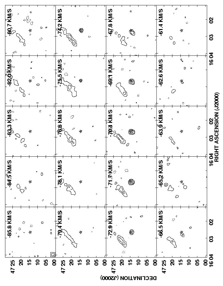
Figure 1: H i channel maps bracketing the LSR velocity of X Her, derived from the Tapered VLA data (see Table 4). A star symbol indicates the position of X Her. Contour levels are (-3,3,6,12)$\times$1.15 mJy beam^-1. The lowest contour is $\sim 3\sigma$. The range of velocities shown corresponds approximately to the range of velocities over which CO(3-2) emission was detected in the CSE of X Her by Knapp et al. 1998. The field-of-view shown is comparable to the VLA primary beam. The size of the synthesized beam is indicated in the lower corner of the upper left panel.

Figure 1 presents selected channel maps from a tapered, naturally weighted VLA H i data cube (see Table 4). The range of velocities shown corresponds approximately to the range over which CO emission has been previously detected in the CSE of X Her (e.g., Knapp et al. 1998). H i emission is detected in all but one of these channels. Toward the position of X Her, we detect H i emission at $\geq 3\sigma$ significance in 10 contiguous channels, ranging in LSR velocity from $-65.2$ km s^-1 to $-76.8$ km s^-1, with the peak emission occurring in the channel centered at $-71.7$ km s^-1. In the same channels, as well as in several additional channels extended toward higher negative velocities, we also detect extended emission to the north and northeast of the star.

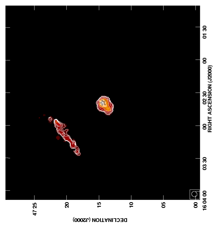
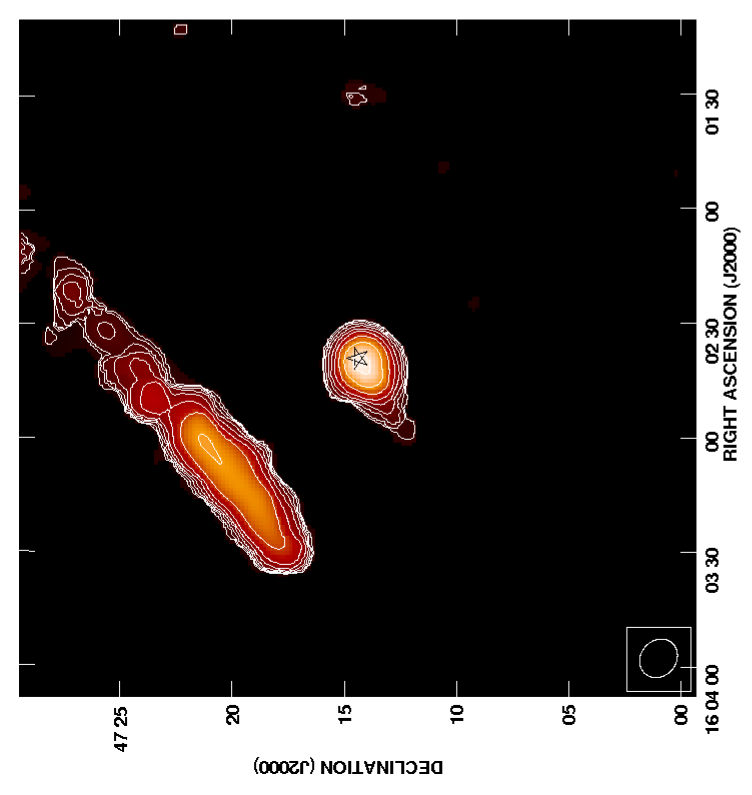
Figure 2: H i total intensity (zeroth moment) maps of X Her derived from the VLA Robust +1 (left) and Tapered data (right) (see Tale 4). Star symbols indicate the position of X Her and the synthesized beam size is indicated in the lower left corner of each panel. Both maps were constructed from emission spanning LSR velocities $-75.5$ to $-65.2$ km s^-1. Intensity levels are 0 to 60 Jy beam^-1 m s^-1 (left) and 0 to 125 Jy beam^-1 m s^-1 (right). Contour levels are (1,1.4,2,…8)$\times$7 Jy beam^-1 (left) and (1,1.4,2,…16)$\times$7 Jy beam^-1 m s^-1 (right). To minimize noise in the maps, data at a given point were blanked if they did not exceed a 2.5$\sigma$ threshold after smoothing by a factor of three spatially and spectrally. The stripe of emission to the northeast is part of a much larger cloud (Cloud I) that does not appear to be directly related to the CSE (see § 7).

The distribution of detected H i emission is further illustrated in Fig. 2, where we show two H i total intensity (moment 0) maps of the region surrounding X Her, derived using two different versions of the VLA data cubes. Spectral channels spanning the velocity range from $-65.2$ km s^-1 to $-75.5$ km s^-1 were used to produce these maps.

In Fig. 2, we see that the emission to the northeast of X Her forms an elongated ridge that appears distinct from the CSE in the VLA data. This ridge is coincident with the direction toward which Gardan et al. (2006) reported evidence of a possible asymmetric outflow from X Her. However, with the VLA we do not detect any adjoining emission between the ridge structure and the emission centered on X Her, suggesting that this material is not directly linked to its CSE. Indeed, as we describe below, our subsequent GBT mapping observations have revealed that the ridge in fact appears to be a local enhancement within a larger H i cloud that lies adjacent (in projection) to the star. We discuss this cloud and its possible origins further below. We focus the remainder of this section on the properties of the H i envelope of X Her as derived from our VLA measurements.

Fig. 2 reveals that the integrated emission toward the position of X Her is significantly extended relative to the synthesized beam. Moreover, the emission exhibits a cometary or “head-tail” morphology, similar to what has been seen previously in the H i envelopes of RS Cnc (Matthews & Reid 2007) and Mira (Matthews et al. 2008). The total extent of the X Her emission as measured from our tapered map (Fig. 2b) is $\sim 6^{\prime}$ (0.24 pc) at a limiting H i column density of $\sim 7.5\times 10^{17}$ atoms cm^-2. The position angle (PA) of the H i “tail” at its outermost measured extent measured from the tapered map is $\sim 121^{\circ}$. However, measurements from the higher resolution map in Fig. 2a yields a PA of $\sim 132^{\circ}$ along the first $\sim 3^{\prime}$ of the tail, indicative of either a curvature or a density asymmetry in the outermost tail material.

The total extent of the H i tail measured by the VLA is approximately a factor of two smaller than the size of the CSE previously derived from IRAS 60$\mu$m measurements ($R_{\rm outer}$=$6^{\prime}\,.2$; Young et al. 1993). This suggests that the CSE may contain even more extended gas to which the VLA is insensitive. This possibility is consistent with our GBT mapping measurements described below (§ 7.2).

In the cases of Mira and RS Cnc, the cometary morphologies of the H i envelopes have been shown to arise from turbulent wakes that are formed as these mass-losing stars barrel through the ISM (Matthews et al. 2008). To evaluate whether a similar scenario can explain the morphology of X Her’s CSE, we have computed the components of the Galactic peculiar space motion of X Her, $(U,V,W)_{\rm pec}$, following the prescription of Johnson & Soderblom (1987). For this calculation we assume a heliocentric radial velocity of $-90.5$ km s^-1, a proper motion in right ascension of $-68.49$ mas yr^-1, and a proper motion in declination of 64.65 mas yr^-1 (van Leeuwen 2007). Correction for the solar motion using the constants of Dehnen & Binney (1998) yields $(U,V,W)_{\rm pec}=(-61,-65,-36)$ km s^-1. Projecting back into an equatorial reference frame yields $(V_{r},V_{\alpha},V_{\delta})_{\rm pec}=(-80,-42,34)$ km s^-1. This implies a space velocity for X Her of $V_{\rm space}\approx 96$ km s^-1 along a position angle of 309^∘. Thus both the position angle of the motion (roughly 180 degrees opposite of the position angle along which the H i tail extends) and the relatively high space velocity of X Her, are consistent with the interpretation of the H i morphology as a gaseous wake trailing the star. The velocity field of the tail material (§ 6.2) further solidifies this interpretation. We note that because the dominant velocity component of X Her is radial, this results in an effective foreshortening of the tail material from our viewing angle. Nonetheless, the tail material contains a record of a significantly extended mass-loss history for X Her (see § 9.1).

6.2 The H i Velocity Field of X Her

6.2.1 Evidence for an Interaction between X Her and the Surrounding ISM

In Fig. 3 we present an H i velocity field derived using the same range of velocities as used to construct the total intensity maps in Fig. 2. The northeastern ridge of emission shows a rather chaotic velocity pattern on these scales. However, across the H i envelope of X Her we see a clear, systematic velocity gradient of $\sim$6.5 km s^-1 along the length of the emission (i.e., a projected gradient $\delta v\sim$35km s^-1 pc^-1). This is further highlighted in Fig. 4, where we plot a position-velocity (P-V) cut extracted along the length of the H i tail. The absolute value of the velocities decrease with increasing distance from the star, which is consistent with deceleration of swept-back wind material owing to its interaction with the surrounding ISM (e.g., Raga & Cantó 2008; hereafter RC08). The same effect has been observed previously in the extended wake of Mira (Matthews et al. 2008).

6.2.2 A Possible Link between the Molecular Outflow and the Atomic Gas in the CSE?

The CO(1-0) observations of Castro-Carrizo et al. (2010) show that the maximum velocity gradient in the molecular outflow (which is confined to $r~{}\hbox to0.0pt{$<$\hss}{\lower 4.30554pt\hbox{$\sim$}}10^{\prime\prime}$) is present along a position angle of $\sim 45^{\circ}$, with blueshifted material to the southwest and redshifted material to the northeast. A closer inspection of the H i velocity field of X Her (Fig. 3) reveals that near the stellar position, the isovelocity contours are somewhat twisted and asymmetric relative to the bisector defined by the trajectory of the star’s motion. A P-V plot extracted from the “robust +1” version of the H i data along the same position angle as the CO outflow (Fig. 5) shows that despite our limited spatial resolution, there is clear evidence for a velocity gradient of $\sim 8\pm 2$ km s^-1 with the same sense as seen in the CO data (i.e., the more blueshifted emission to the southwest). The kinematics of the H i material are consistent with a possible relationship to the molecular outflow, although the axis of symmetry appears to lie near $V_{\rm LSR}\approx-72$ km s^-1 in H i compared with $V_{\rm LSR}\approx-73$ km s^-1 in CO, and the spatial resolution of the H i data is too low to characterize the relationship between the molecular and atomic gas in any detail.

One possibile interpretation of Fig. 5 is that the H i traces a continuation of the molecular outflow beyond the molecular dissociation radius. This would imply that the dynamical age of the outflow is  $>$$\sim$8000 yr (assuming $V_{\rm outflow}=5$ km s^-1). This is roughly an order of magnitude longer than previous estimates based on CO data (cf. Kahane & Jura 1996) and also exceeds by a factor of several or more the typical dynamical ages of the bipolar flows observed in post-AGB stars (e.g., Huggins 2007). Alternatively, the molecular outflow might be a more recent occurrence, with the H i sampling material from a previous (biconical or spherical) mass-loss episode. H i observations with higher spatial and spectral resolution may help to provide additional insight. We note that for the semi-regular variable RS Cnc, which also exhibits a bipolar molecular flow, Libert et al. (2010b) found evidence for an elongation in the H i emission along the molecular outflow direction, again consistent with the possibility of the H i tracing a continuation of the biconical molecular outflow to larger scales.

Establishing the duration over which the mass-loss from X Her has been dominated by a bipolar rather than a spherical wind is relevant to better understanding the CSE properties on large as well as on small scales. For example, Raga et al. (2008) have shown that the presence of a latitude-dependent wind that is misaligned with respect to the direction of motion of a star is expected to impact the large-scale structure of circumstellar wakes. Such an effect could plausibly account for the apparent asymmetry of the tail that we see at larger distances from X Her (see § 6.1). A prolonged bipolar outflow stage would also impact calculations of the time-averaged mass-loss rate from the star, since most mass-loss rates are derived under the assumption of spherically symmetric mass-loss (e.g., Knapp et al. 1998). This would in turn impact the total predicted mass of the H i envelope and tail (see § 9.1).

6.3 The H i Spectrum and Total H i Mass of X Her Based on the VLA Data

We have derived a spatially integrated H i spectrum of X Her from the VLA data by summing the circumstellar emission in each channel image within an irregular “blotch” whose periphery was defined by a 2.5$\sigma$ isophote. Measurements were corrected for the VLA primary beam. The resulting H i spectrum, shown in Fig. 6, exhibits a single-peaked, slightly lopsided shape, similar in shape and breadth to the H i spectra observed for a number of other AGB stars (e.g., Gérard & Le Bertre 2006; Matthews & Reid 2007). Modeling by Gardan et al. (2006) showed that this type of observed asymmetry can be an additional hallmark of a mass-losing star’s interaction with the ISM. For this reason, the spatially integrated H i profile cannot be used to reliably gauge the outflow speed(s) of X Her, as its shape is dominated by the effects of this interaction.

Compared with the mean position-switched NRT spectrum of X Her presented by Gardan et al. (2006), the peak flux density in the spatially-integrated VLA spectrum is $\sim$20% smaller, and the FWHM velocity width ($\sim 5.1\pm 0.6$ km s^-1) is narrower. These differences result in part from our present exclusion of the emission component to the northeast (which has a broader velocity extent than the emission centered on the star; see Fig. 1 and § 7). Based on the VLA data alone, we derive a velocity-integrated H i flux density for X Her of $\int Sd\nu=0.24\pm 0.01$ Jy km s^-1, corresponding to a neutral hydrogen mass of $M_{\rm HI}\approx 1.1\times 10^{-3}~{}M_{\odot}$. However, this value should be regarded as a lower limit, since our VLA maps appear to be missing some extended emission (see § 7.2).

7 Results from the GBT Observations

7.1 Detection of a High-Velocity Cloud in the X Her Field

7.1.1 H i Properties of “Cloud I”

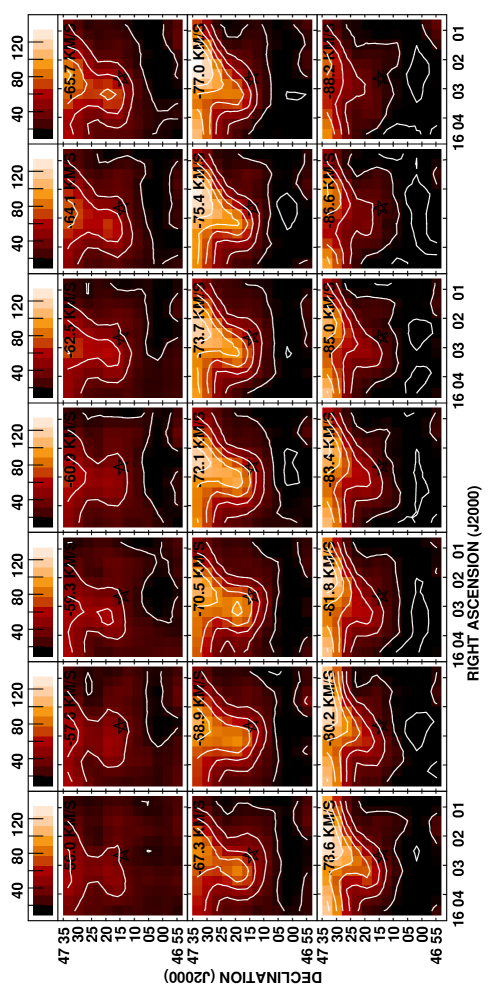
Figure 7: H i channel maps bracketing the velocity of X Her, derived from a GBT grid map of a $\sim 40^{\prime}\times 40^{\prime}$ region around the star. Every third channel is shown within the plotted velocity range. Contour levels are ($-1$,1,3,6,9,12,15,18)$\times$6 mJy beam^-1 and the intensity range is 0 to 140 mJy beam^-1. The lowest contour is $\sim 2\sigma$. The GBT beam has FWHM $\sim 9^{\prime}$ and the pixels are $3^{\prime}\,.5$. These maps reveal that the elongated ridge of emission seen in VLA maps (Fig. 2) is part of a larger cloud lying predominantly north of X Her, but which also extends southward through the position of the star.

Fig. 7 presents selected H i channel maps bracketing the velocity of X Her, as derived from the GBT grid map data. These maps reveal that the elongated ridge of emission seen in our VLA maps (Fig. 2) is part of a much larger-scale cloud of emission, extending outside the VLA primary beam and spreading well beyond the spatial scales of $~{}\hbox to0.0pt{$<$\hss}{\lower 4.30554pt\hbox{$\sim$}}15^{\prime}$ to which the VLA is sensitive. Following Gardan et al. (2006), we hereafter refer to this entity as “Cloud I”. At GBT resolution, the peak emission from Cloud I lies spatially to the northwest of X Her, and spectrally blueward of the stellar systemic velocity. However, the dramatically improved surface brightness sensitivity of the GBT reveals emission extending southward and passing through the position of X Her at all velocities where circumstellar H i was detected with the VLA (viz. $V_{\rm LSR}\sim-66$ to $-77$ km s^-1; Fig. 1). Thus the CSE emission from X Her and the emission from Cloud I are both spatially and spectrally blended in the GBT data.

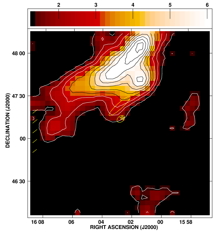
Figure 8: H i total intensity map of the region around X Her, derived from the GBT OTF data, illustrating the morphology of the emission associated with Cloud I. The data were summed over the velocity range $-95.4$ to $-56.0$ km s^-1. The intensity scale has units of Jy m s^-1 and is shown with a logarithmic transfer function. Contour levels are ($-2$[absent],2,3,4…11)$\times$528 Jy m s^-1. The lowest contour level is $\sim 10\sigma$. The yellow ellipses indicate the approximate location and extent of the H i envelope of X Her detected with the VLA, and the ridge of Cloud I emission detected by the VLA, respectively (see Fig. 2). The yellow hatch marks indicate the angles and locations along which the position-velocity cuts shown in Fig. 14 were extracted.

Cloud I clearly extends beyond the northern edge of the GBT grid maps shown in Fig. 7. To more fully illustrate the size and large-scale morphology of the cloud, we therefore show in Fig. 8 an H i total intensity map of the region derived from our GBT OTF mapping data. This latter map appears to contain the bulk of the cloud, although it still does not encompass its northernmost boundary or its eastern tip. Nonetheless, we see that the cloud has an elongated shape, with its brightest regions stretching along a position angle of $\sim 310^{\circ}\pm 5^{\circ}$. Note that the elongated isophotes defining the brightest emission in this map lie to the north of the emission ridge seen in the VLA map in Fig. 2, although both stretch along comparable position angles.

To assess whether Cloud I may have significant additional emission lying outside of our map region, we have examined H i maps extracted from the Leiden/Argentine/Bonn (LAB) Survey (Kalberla et al. 2005) over a several degree region surrounding the position and velocity of Cloud I. The LAB data confirm that our GBT maps have covered the bulk of Cloud I. However, in the LAB maps we find a second compact cloud (hereafter “Cloud II”) near $l^{II}=$$77^{\circ}\,.0$, $b^{II}$=$48^{\circ}\,.5$ with a similar size and peak column density to Cloud I. Cloud II appears well-defined and distinct from Cloud I at contour levels of $T_{\rm B}>0.3$ K, although it blends with Cloud I at lower surface brightness levels. This raises the possibility that both of these clouds could be part of a larger complex (see also Gardan et al. 2006). However, data of higher resolution and sensitivity will be needed to evaluate this possibility and to more thoroughly characterize the properties of Cloud II.

Based on the GBT OTF data for Cloud I, we find that the peak brightness temperature, $T_{\rm B,peak}=0.69$ K, occurs at a position of $\alpha_{\rm J2000}=16^{\rm h}01^{\rm m}13.865^{\rm s}$, $\delta_{\rm J2000}=48^{\circ}06^{\prime}44.76^{\prime\prime}$ and in the spectral channel centered at $V_{\rm LSR}=-80.99$ km s^-1. The Jy to $T_{B}$ conversion factor at the frequency of our observations is 2.21 K Jy^-1. In the velocity-integrated total intensity map presented in Fig. 8, the peak column density is $N_{\rm HI}=2.8\times 10^{19}$ cm^-2.

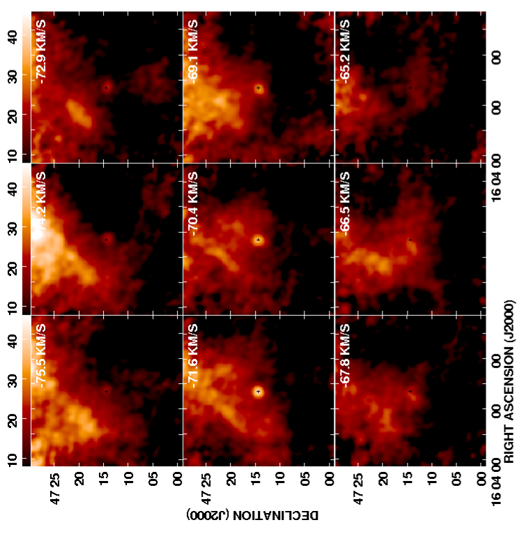
Figure 9: Selected channel maps showing the combined GBT+VLA data across a $\sim 30^{\prime}$ field-of-view. The maps have been corrected for the attenuation of the VLA primary beam. The intensity range is 8 to 45.7 mJy beam^-1. A black cross indicates the position of X Her. LSR velocities are indicated on each panel.

To better illustrate the relationship between the emission seen in the GBT maps and that detected in our VLA imaging, Figure 9 presents several sample channel maps showing the combined VLA+GBT data. These maps reveal that the H i emission from X Her stands out clearly from the larger-scale cloud emission despite their spatial overlap at several positions. These maps also illustrate the relationship between the ridge of emission detected by the VLA to the northeast of X Her and the lower column density emission in the region.

7.1.2 The H i Spectrum of Cloud I

In Fig. 10 we show a spatially integrated H i spectrum of Cloud I derived from the OTF data. Emission in each channel was summed within a fixed $84^{\prime}\times 63^{\prime}$ rectangular aperture, centered at $\alpha_{2000}=16^{h}04^{m}11.5^{s}$, $\delta_{2000}=+47^{\circ}47^{\prime}$$29^{\prime\prime}\,.8$. We see from Fig. 10 (upper panel) that the emission from Cloud I is superposed atop a blue wing extending from the dominant Galactic H i signal along the line-of-sight. The spatially integrated line profile of Cloud I is well fitted by a Gaussian plus a linear background term, resulting in the following global H i line parameters: peak flux density: $F_{\rm peak}=24.8\pm 1.3$ Jy; line centroid: $V_{\rm LSR}=-79.0\pm$0.1 km s^-1; FWHM line width: $\Delta V_{\rm FWHM}=20.0\pm 0.1$ km s^-1. The line centroid thus lies blueward of the stellar systemic velocity of X Her and outside the velocity range over which statistically significant emission was detected from the CSE of the star by the VLA.

Based on the Gaussian fit parameters, we derive an integrated H i line flux for Cloud I $\int S_{\rm HI}d\nu=526$ Jy km s^-1, implying that if it were at the same distance as X Her (140 pc), its total H i mass would be  $>$$\sim$2.4 $M_{\odot}$. This H i mass is a lower limit, since Cloud I appears to extend slightly beyond our map region. Such a quantity of gas is too large to have been shed by X Her alone (whose current mass is estimated to be 1.9 $M_{\odot}$; Table 1), unless this material was significantly augmented by gas swept from the ambient ISM. We discuss the significance of this finding and further constraints on the nature of Cloud I in § 9.2.

7.2 Recovery of Spatially Extended Emission from X Her with the GBT and the Total H i Mass of the CSE

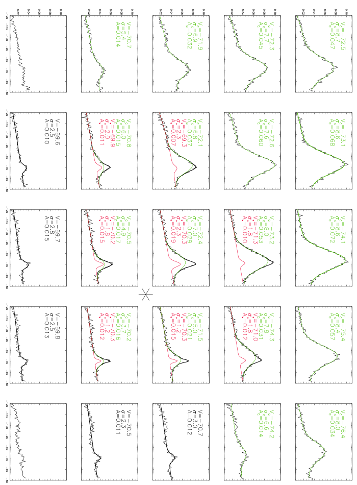
Figure 11: H i spectra extracted through each $3^{\prime}\,.5$ pixel of a 5$\times$5 pixel region of the GBT grid map. Axes are LSR velocity in km s^-1 and flux density in Jy. The position of X Her is indicated by a large asterisk. Overplotted are the results of Gaussian+linear background fits to each spectrum. The component of the emission attributed to Cloud I is indicated by a thin green line and that attributed to the CSE of X Her is indicated by a thin red line. In cases where two components were fitted, the sum is indicated by a thick black line. Finally, for cases where signal-to-noise was insufficient to distinguish between a one- and a two-component fit, a single Gaussian+background fit is overplotted in black. Fit parameters (velocity centroid in km s^-1, dispersion in km s^-1, and amplitude in Jy) for each fitted component are indicated on each panel in a coordinating font color.

Despite the spatial confusion between Cloud I and the circumstellar emission from X Her in the GBT data, we have been able to spectrally isolate the circumstellar signal. Fig. 11 shows a series of one-dimensional spectra, each extracted from a single pixel across a 5$\times$5 pixel portion of the GBT grid map. An asterisk indicates the position of the star. We first attempted to fit each spectrum with a single Gaussian line plus a linear background term. However, for several of the spectra, these fits left statistically significant residuals. We therefore repeated those fits with the inclusion of a second Gaussian component. The results are overplotted on the respective spectra in Fig. 11. The values of the central velocity ($V$), dispersion ($\sigma$), and amplitude ($A$) for each Gaussian component fitted are also indicated.

In Fig. 11 we see that the spectra requiring a second Gaussian component are clustered around the position of X Her. In all of these cases, one spectral component is narrower, of lower amplitude, and (with one exception) systematically redshifted compared with a second, broader line component. Further, the velocities and line widths of these components match well with those derived for the circumstellar emission from X Her based on our VLA data (§ 6.3). We therefore conclude that we have unambiguously detected emission from the CSE of X Her with the GBT.

We note that the FWHM line widths and velocity centroids of the two line components fitted to the spectra in the vicinity of X Her are comparable to those of the “broad” and the “narrow” line components identified by Gardan et al. (2006) in their NRT spectra toward the star. However, our new analysis now reveals that the broader of these two line components appears to be due primarily to Cloud I rather than a northeasterly, asymmetric outflow as originally proposed by Gardan et al. Our present data thus provide no clear evidence for a distinct broad H i component associated with the CSE of X Her.

In Fig. 12 we show a global spectrum for X Her that we derived from the GBT data by summing the spectra from each position in Fig. 11, after subtraction of the background and the emission attributed to Cloud I. The VLA spectrum from Fig. 6 is overplotted for comparison. The peak in the VLA spectrum occurs at slightly lower negative velocities compared with what is seen in the GBT spectrum, but this difference is not statistically significant. Although the FWHM line widths of the two spectra are comparable, the integrated H i line flux derived from the GBT data is $\int Sdv$=0.46 Jy km s^-1, corresponding to $M_{\rm HI}\approx 2.1\times 10^{-3}~{}M_{\odot}$, or roughly twice the value derived from the VLA data. While this value is subject to the uncertainties in the line decompositions of the individual spectra, the significant increase compared with the VLA measurement suggests that the GBT has allowed us to recover extended emission from within the CSE to which the VLA was not sensitive. Moreover, we note that additional emission from the CSE may be present at several of the positions along the lower and right-hand sides of Fig. 11; however, the emission at these locations was too weak to permit an unambiguous decomposition of the line into multiple Gaussian components, and we were thus unable to ascertain whether it arises from the CSE, from Cloud I, or a combination of the two.

While the coarse spatial resolution of our GBT maps make it impossible to determine the overall size of the X Her CSE to great precision, the results presented in Fig. 11 clearly suggest that the CSE is more extended than inferred from our VLA observations alone (§ 6.1). Indeed the H i extent of the CSE now appears to be marginally consistent with the radius $R_{\rm out}$=$6^{\prime}\,.2$ derived from IRAS far-infrared (60$\mu$m) measurements by Young et al. (1993). From the same IRAS measurements, Young et al. derived a mass for the CSE of X Her of $M_{\rm tot}\approx 4\times 10^{-3}~{}M_{\odot}$ (after scaling to our currently adopted distance). If we correct our GBT H i mass for the presence of He, our new total mass estimate of $M_{\rm tot}\approx 3\times 10^{-3}~{}M_{\odot}$ is in reasonable agreement with the far infrared estimate.

7.3 Evidence for Interaction of Cloud I with the ISM

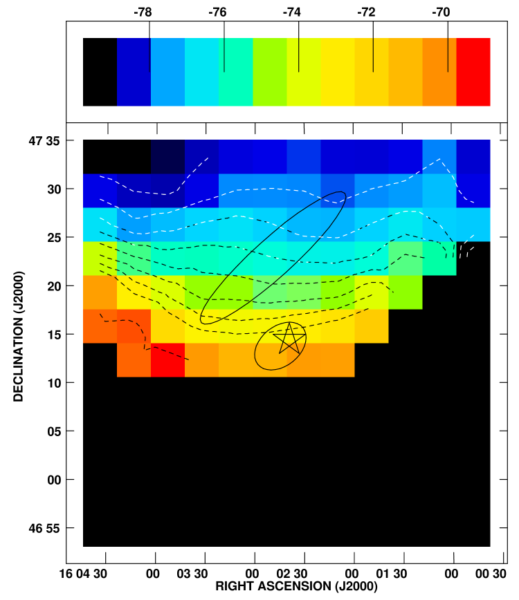
Figure 13: H i velocity field derived from the GBT grid data. The color scale is in units of LSR velocity in km s^-1. Emission in this map is dominated by Cloud I. A systematic velocity gradient is present across the map. The dark ellipses indicate the approximate location and extent of the H i envelope of X Her detected with the VLA, and the ridge of Cloud I emission detected with the VLA, respectively (see Fig. 2).

While isolating the emission from X Her was the original goal of the spectral decompositions of our GBT spectra, an examination of the results as a function of position has revealed an interesting trend (Fig. 11). Near the position of X Her, we find that the centroids of the emission that we attribute to Cloud I (green lines) are redshifted relative to the mean velocity of the cloud ($\approx$80 km s^-1) and differ from X Her by  $<$$\sim$2 km s^-1. However, moving northward, the line centroids of the Cloud I emission become systematically blueshifted, indicating the presence of a systematic velocity gradient across the cloud. This trend is further highlighted in Fig. 13, where we show an H i velocity field derived from the GBT grid data. Emission in this map is dominated by Cloud I. (The signal-to-noise in the OTF data was insufficient to construct a useful first moment map). Interestingly, the direction of the velocity gradient is similar to that within the “tail” of X Her (Fig. 3).

In Fig. 8 we saw that Cloud I has an elongated morphology that extends along a position angle that is similar to the direction of motion of X Her through the ISM (cf. Fig. 3). This, coupled with the presence of a velocity gradient along the direction of elongation, suggests that the material in Cloud I may be influenced by its motion through the ISM. Furthermore, it raises the intriguing possibility that Cloud I and X Her might share a common space motion.

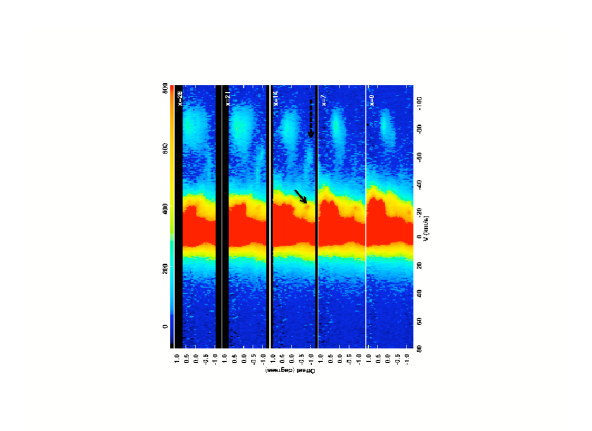
Figure 14: Position-velocity plots, derived at several positions parallel to the long axis of Cloud I (PA=$309^{\circ}$; see Fig. 8). The $y$ axis is the projected distance along the cloud in degrees, with values decreasing toward the southeast (i.e., toward the “tail” of the cloud). The $x$-axis is the LSR velocity. The solid arrow indicates the “compact” feature referred to in the text (§ 7), while the dashed arrow indicates an example of a “streamer” of material that may have been ram pressure stripped from Cloud I. The values in the upper right of each panel indicate the offset in arcminutes (along PA=309^∘) from the southwestern edge of the cloud. The intensity scale is in units of Jy pixel^-1.

To investigate this further, we have examined some P-V cuts extracted at several positions parallel to the long axis of Cloud I, spaced by $\sim 7^{\prime}$. The cut positions are indicated on Fig. 8. We assume a position angle for the cloud of $309^{\circ}$ (the same position angle as the space motion of X Her; see § 6.1). The resulting P-V cuts (Fig. 14) reveal several noteworthy kinematic features. The lower panel of Fig. 14 was extracted near the southwestern edge of the Cloud I, and at this location we see that the emission comprising the cloud (centered near $V_{\rm LSR}=-80$ km s^-1) exhibits an“S”-like shape, indicative of higher negative velocities in the northwest and lower negative velocities toward the southeast. This is consistent with the velocity gradient seen in Fig. 11 & Fig. 13.

In the lower panel of Fig. 14, Cloud I appears to be well-separated from the primary Galactic emission. However, in the subsequent panels ($x\geq 7^{\prime}$), a “bridge” of emission becomes visible, linking Cloud I with the Galactic material. Furthermore, an additional “streamer” appears, stretching along negative velocities to $V_{\rm LSR}\approx-65$ km s^-1. In three of the panels ($x=7^{\prime}$, $x=14^{\prime}$, and $x=21^{\prime}$), this lower streamer appears spatially separated from Cloud I, while in the top panel ($x=28^{\prime}$) it blends smoothly with the lower (southeastern) edge of the cloud. This lower streamer also corresponds in position with a compact feature near $V_{\rm LSR}\approx-$20 km s^-1 (solid arrow on Fig. 14). This compact feature is the most prevalent at $x=14^{\prime}$, but is visible in other P-V cuts as well.

The aforementioned features in the P-V plots along Cloud I strongly support our suggestion that Cloud I has interacted significantly with the ambient ISM. Indeed, we propose that the bridges, streamers, and compact features described above are likely to be the result of material that has been ram pressure stripped from Cloud I as a consequence of its space motion. We discuss the implications of this finding further in § 9.2.

8 Constraints on the Molecular Gas and Dust Properties of Cloud I

8.1 A Search for CO Emission

To obtain additional constraints on the physical properties of Cloud I, we have used the Harvard-Smithsonian 1.2-m millimeter-wave telescope to search for associated ¹²CO $J$=1-0 emission, which would indicate the presence of a denser, molecular component to the cloud. These observations were performed on 2008 March 13.

The observations were obtained using a 256 channel filter bank with 250 kHz (0.65 km s^-1) channel spacing, centered at a velocity $V_{\rm LSR}=-70.0$ km s^-1. The intensity scale was calibrated as described in Dame et al. (2001) and is quoted in units of the main beam brightness temperature. Frequency-switching was employed, with an offset of 15 MHz (39 km s^-1) with a cycle time of 2 seconds.

The 1.2-m telescope has a FWHM beamwidth of $8^{\prime}\,.4$ at 115.2712 GHz (Dame et al. 2001). We obtained a 3$\times$3 grid map with one beamwidth separation between pointings, centered at $(l,b)$=($75^{\circ}\,.92$,+$47^{\circ}\,.78$). The adopted center is near the location of the peak H i column density in Cloud I as inferred from our GBT observations (Fig. 8). Total integration time was $\sim$5 minutes per pointing, resulting in an rms noise of $\sim$0.15 K per channel.

A spectrum derived from the sum of all 9 of our grid pointings is shown in Fig. 15. A sixth order baseline has been fitted and subtracted. The rms noise in this summed spectrum is 0.06 K. No CO emission is evident over the velocity range corresponding to the H i emission from Cloud I (Figure 10). A weak, narrow line is seen slightly outside this window, near $V_{\rm LSR}=-47$ km s^-1, but this feature is most likely spurious, as no conjugate line is seen in the frequency-shifted reference spectrum. (Such a line would appear as an apparent “absorption” feature near $V_{\rm LSR}=-8$ km s^-1 in the frequency-differenced spectrum shown in Fig. 15).

To place an upper limit on the column density of molecular gas in the core of Cloud I, we assume a fiducial CO line width of 5 km s^-1 and a Galactic CO-to-H₂ conversion factor of $X=N_{H_{2}}/\int T_{\rm mb}({\rm CO})dV=1.8\times 10^{20}$ cm^-2 K^-1 (km s^-1)^-1 (Dame et al. 2001). This translates to a 3$\sigma$ upper limit on the H₂ column density of $N_{H_{2}}<1.3\times 10^{20}$ cm^-2.

The lack of CO emission toward Cloud I is consistent with its modest peak H i column density, as well as the lack of detected CO emission from other H i clouds with similar properties (Wakker et al. 1997; Dessauges-Zavadsky et al. 2007). As discussed below, Cloud I exhibits properties consistent with a high-velocity cloud, which are typically undetected in CO, with the exception of a handful of examples that appear to be associated with tracers of past or ongoing massive star formation (Désert et al. 1990; Oka et al. 2008).

8.2 A Search for Far-Infrared Emission from Cloud I

Using the IRAS-IRIS images (Miville-Deschênes & Lagache 2005), obtained via the IRAS archive (http://irsa.ipac.caltech.edu), we have searched for FIR (60$\mu$m) emission associated with Cloud I. While IRAS clearly detects patches of diffuse FIR emission overlapping in position with Cloud I, we find no obvious correspondence between either the morphology or the surface brightness of the FIR emission and the column density of the H i emission in the region. In particular, the ridge of emission exhibiting the highest H i column density in Fig. 8 does not have any obvious FIR counterpart. Moreover, most of the H i emission that could plausibly be associated with FIR emission in the region around X Her and Cloud I has $V_{\rm LSR}\approx$0 km s^-1 (i.e., near the peak of the Galactic emission), not near $V_{\rm LSR}\approx-$80 km s^-1. We conclude that based on present data, there is no compelling evidence for a warm dust component associated with Cloud I.

9 Discussion

9.1 The Age of X Her’s Tail and the Implications for its Mass-Loss History

As described in Matthews et al. (2008), the kinematic information supplied by H i observations of circumstellar wakes is particularly valuable for estimating their ages, and hence the overall duration of the AGB mass-loss phase. Furthermore, the recent work by RC08 provides an elegantly simple approach to computing the mass-loss duration, even for the case where the deceleration of the wake material is non-uniform, as appears to be the case for X Her (see Fig. 4).

To estimate the age of X Her’s tail, we adopt a reference frame in which the star is stationary, and the ISM appears to stream past it (see Fig. 2 of RC08). To perform this calculation, we have first deprojected the distances along the $x$-axis of Fig. 4 and the measured radial velocities along the H i tail ($y$-axis of Fig. 4) into the X Her rest frame using the space velocity vectors derived in § 6.1. A subsequent fit to the resulting velocity versus position curve yields the polynomial coefficients $a=0.09\pm 0.01$ and $d=1.5\pm 0.1$ pc (see Eq. 5 of RC08), which in turn define an analytic law describing $[V_{\rm space}-v(x)]$, where $V_{\rm space}$ is the space velocity of the star (or equivalently, the streaming velocity of the ISM in the stellar rest frame), and $v(x)$ is the average axial velocity along the tail at a distance $x$ from the star. Finally, one may express the age of the tail as $t_{\rm tail}=\int^{x_{0}}_{0}[V_{\rm space}-v(x)]^{-1}dx$, where we have taken $x_{0}$=0.32 pc as the maximum (deprojected) distance along the tail at which we were able to reliably measure the gas velocity. From this approach, we find $t_{\rm tail}\approx 1.2\times 10^{5}$ yr. This new estimate for the mass-loss duration of X Her exceeds by roughly a factor of three the value previously derived by Young et al. (1993) using infrared measurements, and it approaches the expected interval between thermal pulses for AGB stars (cf. Vassiliadis & Wood 1993).

Sources of uncertainty in our age estimate for the tail arise first, from the uncertainty in its deprojected length, $x_{0}$, owing to errors on the stellar parallax (5%; van Leeuwen 2007) and the proper motions ($\sim$1%; Perryman et al. 1997). A dominant source of uncertainty in the space velocity of X Her arises from uncertainties in the adopted solar constants (see § 6.1), for which we estimate an error contribution of $\sim\pm$5 km s^-1, or 5%, to each of the equatorial components of the space velocity. The total formal error on $t_{\rm tail}$ is then $\sim$10%. Lastly, the uncertainties in the coefficients of our polynomial fit contribute an additional uncertainty in the age of $\sim$10%. Combining the above values, we therefore estimate the global uncertainty in $t_{\rm tail}$ to be $\sim$20%. We note also that our age estimate depends implicitly on the assumption that the ambient ISM does not exhibit any local flows in the vicinity of X Her.

If we adopt a mass-loss rate for X Her of $\dot{M}=1.44\times 10^{-7}~{}M_{\odot}$ yr^-1 (Table 1), our derived age predicts that the total mass of the CSE of X Her should be $\sim 0.017M_{\odot}$, or roughly 6 times greater than we have inferred from our H i measurements after correction for He (§ 7.2). One explanation for this discrepancy is that a significant fraction of the CSE of X Her comprises molecular rather than atomic hydrogen. However, given the effective temperature of the star ($T_{\rm eff}\approx$ 3281 K), the models of Glassgold & Huggins (1983) predict that the wind should be predominantly atomic as it leaves the star. This possibility therefore seems unlikely, unless there exists a mechanism by which efficient H₂ formation can occur within the tail (see also Ueta 2008).

A second possibility is that we have attributed too large a fraction of the H i emission in the vicinity of the star to Cloud I. However, fully reconciling our H i data with the above mass prediction would require that all of the emission detected by the GBT in the vicinity of X Her (i.e., within panels 2, 3, and 4 of the lower three rows of Fig. 11) is associated with its CSE. This extreme scenario seems unrealistic since Fig. 9 shows clear evidence for spatial overlap between stellar and cloud emission. Further, we note that a total CSE mass of $\sim 0.017~{}M_{\odot}$ would require a highly unusual gas-to-dust ratio to reconcile it with the FIR measurements of Young et al. (1993).

A third conceivable explanation for the above discrepancy is that the mass-loss rate from X Her has not remained constant over the past $\sim 10^{5}$ yr. Indeed, the map shown in Fig. 2b shows that the H i tail tapers to a significantly narrower shape with increasing distance from the star, consistent with a lower past mass-loss rate. Furthermore, our age estimate for X Her predicts that the star should have undergone at least one thermal pulse, after which the mass-loss rate is predicted to decrease by roughly an order of magnitude (Vassiliadis & Wood 1993). Unfortunately, direct evidence for time-variable mass-loss (e.g., in the form of density variations in the tail material) is difficult to infer from the present H i data because of their limited spatial resolution. Moreover, the hydrodynamic simulations of Wareing et al. (2007) have shown that such effects are likely to be difficult to distinguish from density variations in the tail resulting from turbulent effects.

Finally, we should consider the overall uncertainty in the stellar mass-loss rate, independent of whether this rate has been time-variable. Mass-loss rates derived for X Her by different workers based on SiO or CO data exhibit a dispersion of $\sim$15% (e.g., Table 2). However, the uncertainties inherent in various model assumptions imply that a more realistic estimate of the overall uncertainty in the mass-loss rates could be as high as a factor of two (see e.g., Olofsson et al. 2002). This could conceivably account for part of the discrepancy between our measured and predicted values for the tail mass of X Her. However, an additional complication is that all of the mass-loss rates in Table 2 were derived under the assumption of spherically symmetric mass-loss. To our knowledge, Kahane & Jura (1996) are the only authors to have derived a mass-loss rate for X Her that takes into account the bipolar nature of its molecular outflow (§ 2.2). When scaled to our currently adopted distance, the mass-loss rate of Kahane & Jura is comparable to or higher than the values quoted in Table 2 [i.e., $(1.4-3.4)\times 10^{-7}M_{\odot}$ yr^-1, depending on the adopted inclination], which could make the “missing mass” problem even more severe.

9.2 The Origin and Nature of Cloud I and its Possible Relationship to X Her

We summarize in Table 5 some properties of Cloud I as derived in the preceding sections. It is noteworthy that in terms of several of its global properties (H i linewidth, peak H i column density, and peak brightness temperature) Cloud I shows a striking similarity to the so-called “compact high-velocity clouds” (CHVCs; Braun & Burton 1999). The CHVCs represent a distinct subset of HVCs that are physically compact (FWHM$\leq 2^{\circ}$) and sharply bounded in angular extent down to very low column densities ($N_{\rm HI}\approx 1.5\times 10^{18}$ cm^-2; de Heij et al. 2002a). Based on a sample of 179 CHVCs, Putman et al. (2002) reported mean values of $\Delta V_{\rm FWHM}$=35 km s^-1, $N_{\rm HI}=1.4\times 10^{19}$ cm^-2, and $T_{\rm peak}$=0.2 K, respectively, comparable to values in Table 5. The integrated H i flux of Cloud I is significantly larger than the mean value of 19.9 Jy km s^-1 reported by Putman et al., suggesting that it may have a smaller distance than most CHVCs, although it still lies within the range of reported values (see also de Heij et al. 2002c). Finally, like Cloud I, nearly all CHVCs discovered to date exhibit distinctly non-spherical shapes, which are frequently consistent with ram pressure effects as the clouds transverse the ambient medium (Brüns & Westmeier 2004).

Table 5: Properties of Cloud I

Parameter	Value	Comment
$\alpha$ (J2000.0)	16 01 13.86	$a$
$\delta$ (J2000.0)	48 06 44.76	$a$
$l$	$75^{\circ}\,.81$	$a$
$b$	$+47^{\circ}\,.84$	$a$
$T_{B}$ (peak)	0.69 K	$b$
$N_{\rm HI}$ (peak)	2.8$\times 10^{19}$ cm-2	$c$
$\int S_{\rm HI}d\nu$	526 Jy km s-1	$d$
$M_{\rm HI}$	$>1.22\times 10^{-4}d^{2}_{*}~{}M_{\odot}$	$d$,$e$
$V_{\rm LSR}$	$-79.0\pm 0.1$ km s-1	$d$
$\Delta V_{\rm FWHM}$	20$\pm 0.1$ km s-1	$d$
Angular Size	$\sim 2^{\circ}$	…
$T_{k}$	$\leq$7750 K	$f$
$N_{H_{2}}$	$<1.3\times 10^{20}$ cm-2	$g$

.

Note. — Tabulated parameters are uncorrected for possible emission extending beyond our survey region.

Cloud I is not included in existing CHVC catalogues (de Heij et al. 2002b; Putman et al. 2002), as it lies just outside the velocity cutoff searched in previous surveys ($|V_{\rm LSR}|>$90 km s^-1; Putman et al. 2002). Adoption of such cutoffs in HVC surveys is necessary to minimize contamination and confusion by unrelated Galactic disk emission. However, as pointed out by de Heij et al. (2002c), any reasonable model for CHVCs predicts that examples should also be found at less extreme velocities. The properties of Cloud I together with its high Galactic latitude suggest that it is one such example. For this reason, we resist terming Cloud I instead as an “intermediate velocity cloud” (IVC; see Wakker 2004), particularly since some evidence suggests that many IVCs are linked with energetic phenomena such as supernovae and may form a population largely distinct from the HVCs (Désert et al. 1990; Kerton et al. 2006).

Uncovering the nature of Cloud I is complicated by the uncertainty in its distance. A plausible lower limit for the cloud would be that it is at the same distance as X Her ($\sim$140 pc). If we assume that the cloud consists primarily of neutral atomic material (§ 8.1), then at this short distance its total mass would be only $M_{\rm tot}\sim 3.4M_{\odot}$ (where we have used a factor of 1.4 to correct the measured H i flux density for the mass of He). As we noted in § 7.1.2, this quantity of material excludes the possibility of an origin tied directly to the mass-loss from X Her unless the material was augmented significantly from debris swept from the ambient ISM. Moreover, such a scenario would require a differential acceleration between Cloud I and X Her such that Cloud I now has a larger blueshifted velocity compared with X Her.

Based on its morphology and kinematics, Cloud I is almost certainly not virialized; indeed, an implausibly large distance of $\sim$2 Mpc would be required in order that its virial mass, $M_{\rm vir}=\sigma^{2}r/G$, equal its H i mass, assuming a local velocity dispersion $\sigma\sim$8 km s^-1 (see Fig. 11). Here $r$ is the radius of the cloud and $G$ is the gravitational constant.

One further constraint on the distance to Cloud I can be estimated from our present data by assuming that Cloud I has interacted with material near its present location that follows the “normal” Galactic rotation pattern (see also Lockman et al. 2008). From Fig. 14, we see signatures of perturbations in material at velocities as high as $V_{\rm LSR}~{}\hbox to0.0pt{$<$\hss}{\lower 4.30554pt\hbox{$\sim$}}-10$ km s^-1. Following Reid et al. (2009), the kinematic distance to material at this position and velocity is $\sim 4.98^{+0.71}_{-0.82}$ kpc. Unfortunately, kinematic distance determinations toward the direction of Cloud I are highly uncertain, and changes of only a few km s^-1 in the assumed LSR velocity can translate to a significant change in the implied kinematic distance. For example, taking instead $V_{\rm LSR}=0$ km s^-1 (the mean Galactic velocity toward this direction) implies either a “near” distance of 0.430${}^{+4.21}_{-0.43}$ kpc (consistent with X Her to within the large uncertainties) or a “far” distance of 3.66${}^{+0.98}_{-0.98}$ kpc. We conclude that while kinematic arguments suggest a rough upper limit to the distance to Cloud I of $\sim$5 kpc, they cannot yet exclude the possibility of a comparable distance for Cloud I and X Her. Future stellar absorption line measurements toward Cloud I and/or a search for associated diffuse H$\alpha$ emission may help to provide additional distance constraints.

As with the “near” distance for Cloud I discussed above, assumption of the “far” distance would seem to lead to some puzzling inconsistencies. For example, at a distance of 5 kpc, Cloud I would have an H i mass of $\sim 3.1\times 10^{3}~{}M_{\odot}$ and a linear extent of $\sim$170 pc, which are both consistent with upper limits derived for CHVCs under the assumption that they reside in the Galactic halo (Westmeier et al. 2005). On the other hand, this would require that X Her and Cloud I are related only by a chance superposition along the line-of-sight—a circumstance with a rather low statistical probability. Putman et al. (2002) found that the covering fraction for CHVCs is only $\sim$1%. Furthermore, toward a given Galactic longitude, a typical dispersion in the observed distribution of velocities is $\sim$100 km s^-1 (see Fig. 20 of Putman et al.). Based on these statistics, we estimate the probability of a chance superposition of a CHVC along the line-of-sight to X Her, having a peak velocity within $\pm$10 km s^-1 of the star, is approximately 0.2%. While this estimate ignores possible clustering of CHVCs and does not account for incompleteness of present surveys, finding an apparent space motion for the cloud along the same direction as the star’s space motion makes the coincidence even more remarkable.

One possible explanation for a CHVC in the vicinity of one or more evolved, mass-losing stars is if both have been stripped from a globular cluster. For example, van Loon et al. (2009) have identified a CHVC-like cloud in the vicinity of the globular Pal 4 and have shown that a link between the two is plausible. However, the proximity of X Her to the Sun and the Galactic Plane suggest that it is likely to be a disk object and therefore unlikely to have originated in a globular cluster.

10 Summary

We have presented H i 21-cm line observations of the CSE of the semi-regular variable star X Her. X Her was previously detected in H i by Gardan et al. (2006), but our new observations have allowed us to characterize the morphology and kinematics of the emission in significantly greater detail. We find that the H i emission comprises an extended, cometary-shaped wake that results from the motion of this mass-losing star through the ISM. We estimate the total deprojected extent of the extended CSE to be $\geq$0.3 pc. Analogous H i wakes have now been found associated with other AGB stars including RS Cnc (Matthews & Reid 2007) and Mira (Matthews et al. 2008), and evidence is accumulating that they may be quite common around mass-losing stars, particularly those with high space velocities.

We detect a radial velocity gradient along the H i tail of X Her of $\sim$6.5 km s^-1 ($\delta v\sim$35 km s^-1 pc^-1), indicating a deceleration of the circumstellar gas owing to its interaction with the ambient ISM. Based on the observed deceleration, we estimate an age for the tail of $\sim 1.2\pm 0.3\times 10^{5}$ years, implying a mass-loss history for the star several times longer than the previous empirical estimate. However, the total H i mass that we measure for the tail ($M_{\rm HI}\approx 2.1\times 10^{-3}~{}M_{\odot}$) is significantly smaller than predicted given this age and the current mass-loss rate of the star derived from CO observations. One explanation is that the mass-loss rate of the star has not been constant and has been increasing with time. Another is that a significant portion of the tail material is in the form of molecular hydrogen.

Previous CO observations of X Her have established the existence of a bipolar outflow extending to $\sim\pm 10^{\prime\prime}$ along a position angle of 45^∘ (e.g., Castro-Carrizo et al. 2010). Along this position angle, we have detected a velocity gradient in the H i emission similar to the one seen in CO, suggesting that the bipolar outflow may extend to at least $\sim\pm 1^{\prime}$ from the star and have a dynamical age much larger than previously estimated ( $>$$\sim$8000 yr). An alternative is that the H i may be tracing an earlier mass-loss episode.

X Her lies (in projection) along the periphery of a more massive and extended H i cloud (Cloud I), whose radial velocity overlaps with that of the CSE of X Her. Emission from this cloud can account for the apparent asymmetric mass-loss from X Her previously reported by Gardan et al. (2006). We have characterized the H i properties of Cloud I in detail and find them to be similar to those of CHVCs. Using ¹²CO observations, we have also placed an upper limit on the molecular gas content of the cloud of $N_{H_{2}}<1.3\times 10^{20}$ cm^-2. In our H i observations, we see evidence of a velocity gradient along Cloud I, suggesting that like X Her, its morphology and kinematics are affected by its motion through the ambient ISM. Both the high mass of Cloud I ($M_{\rm HI}~{}\hbox to0.0pt{$>$\hss}{\lower 4.30554pt\hbox{$\sim$}}2.4~{}M_{\odot}$) and the blueshift of its mean velocity relative to X Her appear to rule out a direct circumstellar origin. However, the probability of a mere chance superposition in position, velocity, and direction of space motion between Cloud I and X Her is extremely low. Therefore a kinematic association between the two objects cannot yet be excluded and awaits more robust distance constraints for the cloud.

Figure 3: H i velocity field of X Her, derived from the VLA Tapered data. The direction of X Her’s space motion is indicated by an arrow. Colors indicate radial velocity (LSR frame) in km s^-1. A systematic velocity gradient is seen along the emission trailing opposite to the direction of motion of X Her.

Figure 4: H i position-velocity cut along the “tail” of X Her derived from VLA data. The cut was extracted along a position angle of 309^∘. The plotted quantities are uncorrected for projection effects; distances are measured in the plane of the sky and velocities are along the line-of-sight.

Figure 5: H i position-velocity plot for X Her, extracted along a position angle of 45^∘ from the “robust +1” data (Table 4). The stellar systemic velocity is $V_{\rm LSR}\approx-73$ km s^-1, and spatial offsets along the $x$-axis increase to the northeast. A bipolar outflow with an extent of $\sim\pm 10^{\prime\prime}$ has been seen along this direction in previous CO observations. The H i emission extends over larger spatial scales, but exhibits a velocity gradient of comparable sign and magnitude to the CO emission. Contour levels are ($-2$,2,4,6,8,10,12)$\times 1.0$ mJy beam^-1.

Figure 6: Spatially integrated H i spectrum of X Her derived from the VLA data.

Figure 10: Spatially integrated H i spectra of Cloud I derived from GBT OTF data (see Text). The upper panel shows a zoom of the spectral region around Cloud I. The systemic velocity of X Her is indicated by a vertical line. A fit to the Cloud I line profile with a Gaussian plus linear background is overplotted as a thick line. The lower panel shows the same data over a broader velocity range. The dominant Galactic emission toward this direction peaks near $V_{\rm LSR}\approx$0 km s^-1. The spikes near 85 and 110 km s^-1 are due to RFI.

Figure 12: Global H i spectrum of X Her derived from the GBT grid data (solid line). The spectrum was derived by summing the seven spectra from Fig. 11 where circumstellar emission could be unambiguously identified. The emission contributions from Cloud I plus a linear background term were subtracted from each spectrum before summation. The VLA spectrum from Fig. 6 is overplotted as a dashed line.

Figure 15: ¹²CO $J$=1-0 spectrum toward the position of peak H i column density in Cloud I. Nine frequency-switched spectra covering a 3$\times$3 beam grid with $8^{\prime}\,.4$ spacings, centered at $(l,b)=$($75^{\circ}\,.92$,$+47^{\circ}\,.78$) have been averaged (see § 8.1).

References

- (1) Bowers, P. F. & Knapp, G. R. 1988, ApJ, 332, 299
- (2) Braun, R. & Burton, W. B. 1999, A&A, 341, 437
- (3) Briggs, D. S. 1995, Ph.D. Thesis, New Mexico Institute of Mining and Technology
- (4) (http://www.aoc.nrao.edu/dissertations/dbriggs/)
- (5) Brüns, C. & Westmeier, T. 2004, A&A, 426, L9
- (6) Castro-Carrizo, A., Quintana-Lacaci, G., Neri, R., Bujarrabal, V., Schöier, F. L., Winters, J. M., Olofsson, H., Lindqvist, M., Alcolea, J., Lucas, R., & Grewing, M. 2010, A&A, in press
- (7) Condon, J. J., Cotton, W. D., Greisen, E. W., Yin, Q. F., Perley, R. A., Taylor, G. B., & Broderick, J. J. 1998, AJ, 115, 1693
- (8) Cristallo, S., Straniero, O. Gallino, R., Piersanti, L., Domínguez, I., & Lederer, M. T. 2009, ApJ, 696, 797
- (9) Dame, T. M., Hartmann, D., & Thaddeus, P. 2001, ApJ, 547, 792
- (10) de Heij, V., Braun, R., & Burton, W. B. 2002a, A&A, 391, 67
- (11) de Heij, V., Braun, R., & Burton, W. B. 2002b, A&A, 391, 159
- (12) de Heij, V., Braun, R., & Burton, W. B. 2002c, A&A, 392, 417
- (13) Dehnen, W. & Binney, J. 1998, MNRAS, 298, 387
- (14) Désert, F.-X., Bazell, D., & Blitz, L. 1990, ApJ, 355, L51
- (15) Dessauges-Zavadsky, M., Combes, F., & Pfenniger, D. 2007, A&A, 473, 863
- (16) D’Odorico, S., Benvenuti, P., Dennefeld, M., Dopita, M. A., & Greve, A. 1980, A&A, 92, 22
- (17) Dumm, T. & Schild, H. 1998, New Astron., 3, 137
- (18) Dyck, H. M., van Belle, G. T., & Thompson, R. R. 1998, AJ, 116, 981
- (19) Gardan, E., Gérard, E., & Le Bertre, T. 2006, MNRAS, 365, 245
- (20) Gérard, E. & Le Bertre, T. 2006, AJ, 132, 2566
- (21) Glassgold, A. E. & Huggins, P. J. 1983, MNRAS, 203, 517
- (22) González Delgado, D., Olofsson, H., Kerschbaum, F., Schöier, F. L., Lindqvist, M., & Groenewegen, M. A. T. 2003, A&A, 411, 123
- (23) Hinkle, K. H., Lebzelter, T., Joyce, R. R., & Fekel, F. C. 2002, AJ, 123, 1002
- (24) Huggins, P. J. 2007, ApJ 663, 342
- (25) Huggins, P. J., Mauron, N., & Wirth, E. A. 2009, MNRAS, 396, 1805
- (26) Isaacman, R. 1979, A&A, 77, 327
- (27) Johnson, D. R. H. & Soderblom, D. R. 1987, AJ, 93, 864
- (28) Kahane, C. & Jura, M. 1996, A&A, 310, 952
- (29) Kalberla, P. M. W., Burton, W. B., Harmann, D., Arnal, E. M., Bajaja, E., Morras, R., & Pöppel, W. G. L. 2005, A&A, 440, 775
- (30) Kerschbaum, F., Olofsson, H., & Hron, J. 1996, A&A, 311, 273
- (31) Kerton, C. R., Knee, L. B. G., & Schaeffer, A. J. 2006, AJ, 131, 1501
- (32) Kiss, L. L., Szatmáry, K., Cadmus, R. R. Jr., & Mattei, J. A. 1999, A&A, 346, 542
- (33) Knapp, G. R., Young, K., Lee, E., & Jorissen, A. 1998, ApJS, 117, 209
- (34) Ladjal, D. et al. 2010, A&A, 518, L141
- (35) Libert, Y., Gérard, E., & Le Bertre, T. 2007, MNRAS, 380, 1161
- (36) Libert, Y., Le Bertre, T., Gérard, E., & Winters, J. M. 2008, A&A, 491, 789
- (37) Libert, Y., Gérard, E., Thum, C., Winters, J. M., Matthews, L. D., & Le Bertre, T. 2010a, A&A, 510, 14
- (38) Libert, Y., Winters, J. M., Le Bertre, T., Gérard, E., & Matthews, L. D. 2010b, A&A, 515, A112
- (39) Lockman, F. J., Benjamin, R. A., Heroux, A. J., & Langston, G. I. 2008, ApJ, 679, L21
- (40) Loup, C., Forveille, T., Omont, A., & Paul, J. F. 1993, A&AS, 99, 291
- (41) Lu, P. K., Demarque, P., van Altena, W., McAlister, H., & Hartkopf, W. 1987, AJ, 94, 1318
- (42) Mangum, J. G., Emerson, D. T., & Greisen, E. W. 2007, A&A, 474, 697
- (43) Martin, D. C. et al. 2007, Nature, 448, 780
- (44) Matthews, L. D. & Reid, M. J. 2007, AJ, 133, 2291
- (45) Matthews, L. D., Libert, Y., Gérard, E., Le Bertre, T., & Reid, M. J. 2008, ApJ, 684, 603
- (46) Miville-Deschênes, M-A. & Lagache, G. 2005, ApJS, 157, 302
- (47) Morris, M. & Jura, M. 1983, ApJ, 264, 546
- (48) Nakashima, J.-I. 2005, ApJ, 620, 943
- (49) Olofsson, H., González Delgado, D., Kerschbaum, F., & Schöier, F. L. 2002, A&A, 391, 1053
- (50) Oka, T., Hasegawa, T., White, G. J., Sato, F., Tsuboi, M., & Miyazaki, A. 2008, PASJ, 60, 429
- (51) Perley, R. A. & Taylor, G. B. 2003, VLA Calibration Manual
- (52) (http://www.vla.nrao.edu/astro/calib/manual/index.shtml)
- (53) Perryman, M. A. C. et al. 1997, A&A, 323, L49
- (54) Putman, M. E. et al. 2002, AJ, 123, 873
- (55) Raga, A. C. & Cantó, J. 2008, ApJ, 685, L141 (RC08)
- (56) Raga, A. C., Cantó, J., De Colle, F., Esquivel, A., Kajdic, P., Rodríguez-González, A., & Velázquez, P. F. 2008, ApJ, 680, L45
- (57) Reid, M. J. et al. 2009, ApJ, 700, 137
- (58) Sahai, R. & Chronopoulos, C. K. 2010, ApJ, 711, L53
- (59) Sahai, R. & Wannier, P. G. 1992, ApJ, 394, 320
- (60) Serabyn, E., Lacy, J. H., & Achtermann, J. M. 1991, ApJ, 378, 557
- (61) Smith, H. 1976, MNRAS, 175, 419
- (62) Stencel, R. E. 2009, in The Biggest, Baddest, Coolest Stars, ASP Conf. Series, Vol. 412, ed. D. G. Luttermoser, B. J. Smith, & R. E. Stencel, 197
- (63) Ueta, T. et al. 2006, ApJ, 648, L39
- (64) Ueta, T. 2008, ApJ, 687, L33
- (65) Ueta, T. et al. 2010a, to appear in AKARI, a Light to Illuminate the Misty Universe, preprint (astro-ph/0905.0756)
- (66) Ueta, T. et al. 2010b, A&A, 514, 16
- (67) van Leeuwen, F. 2007, A&A, 474, 653
- (68) van Loon, J. T., Stanimirović, S., Putman, M. E., Peek, J. E. G., Gibson, S. J., Douglas, K. A., & Korpela, E. J. 2009, MNRAS, 396, 1096
- (69) Vassiliadis, E. & Wood, P. R. 1993, ApJ, 413, 641
- (70) Villaver, E., García-Segura, G., & Manchado, A. 2002, ApJ, 571, 880
- (71) Villaver, E., García-Segura, G., & Manchado, A. 2003, ApJ, 585, L49
- (72) Villaver, E., García-Segura, G., & Manchado, A. 2004, RevMexAA, 22, 140
- (73) Wakker, B. P. 2004, in High-Velocity Clouds, ed. H. van Woerden et al. (Dordrecht: Kluwer), 25
- (74) Wakker, B. P., Murphy, E. M., van Woerden, H., & Dame, T. M. 1997, ApJ, 488, 216
- (75) Wallerstein, G. & Dominy, J. F. 1988, ApJ, 326, 292
- (76) Wareing, C. J., O’Brien, T. J., Zijlstra, A. A., Kwitter, K. B., Irwin, J., Wright, N., Greimel, R., & Drew, J. E. 2006a, MNRAS, 366, 387
- (77) Wareing, C. J., Zijlstra, A. A., & O’Brien, T. J. 2007a, ApJ, 660, L129
- (78) Wareing, C. J., Zijlstra, A. A., & O’Brien, T. J. 2007b, MNRAS, 382, 1233
- (79) Wareing, C. J., Zijlstra, A. A., O’Brien, T. J., Seibert, M. 2007c, ApJ 670, L125
- (80) Wareing, C. J., et al. 2006b, MNRAS, 372, L63
- (81) Westmeier, T., Brüns, C., & Kerp, J. 2005, in Extraplanar Gas, ASP Conf. Series, ed. R. Braun, (ASP: San Francisco), 105
- (82) Williams, D. R. W. 1973, A&AS, 8, 505
- (83) Young, K., Phillips, T. G., & Knapp, G. R. 1993, ApJ, 409, 725
- (84) Zijlstra, A. A. & Weinberger, R. 2002, ApJ, 572, 1006