Interplay between Lattice Distortion and Spin-Orbit Coupling in Double Perovskites

Abstract

We develop anisotropic pseudo-spin antiferromagnetic Heisenberg models for monoclinically distorted double perovskites. We focus on these A₂BB^′O₆ materials that have magnetic moments on the $4d$ or $5d$ transition metal B^′ ions, which form a face-centered cubic lattice. In these models, we consider local $z$-axis distortion of B^′-O octahedra, affecting relative occupancy of $t_{2g}$ orbitals, along with geometric effects of the monoclinic distortion and spin-orbit coupling. The resulting pseudo-spin-$1/2$ models are solved in the saddle-point limit of the Sp($N$) generalization of the Heisenberg model. The spin $S$ in the SU(2) case generalizes as a parameter $\kappa$ controlling quantum fluctuation in the Sp($N$) case. We consider two different models that may be appropriate for these systems. In particular, using Heisenberg exchange parameters for La₂LiMoO₆ from a spin-dimer calculation, we conclude that this pseudo-spin-$1/2$ system may order, but will be very close to a disordered spin liquid state.

I Introduction

Geometrically frustrated magnets have been of great recent interest, and are a common starting point in search of exotic ground states.moessnerfrustration ; greedanfrustration One class of such frustrated antiferromagnets is found in the double perovskite oxides, which host a wide range of interesting behavior.ericksonBaNaOsO ; krockenbergermogare ; battleBaYRuO ; kobayashiSrFeMoO ; rameshmultiferroic ; katoreperovskites These compounds of chemical formula A₂BB^′O₆ feature ordered, interpenetrating face-centered cubic (FCC) lattices of the B and B^′ ions when the charge difference between these ions is large.andersondperov Both B and B^′ transition metal ions are octahedrally coordinated by oxygen. A geometrically frustrated FCC lattice is obtained when only the B^′ ions are magnetic.

A conventional picture of isotropic antiferromagnetic superexchange is insufficient for these materials. Altering this picture are two important effects considered in our work. The first effect is spin-orbit coupling, which is relevant for the $4d$ and $5d$ transition metal ions that comprise the magnetic sites. Spin-orbit coupling has been seen to lead to increased correlation effects, particularly in materials containing $5d$ Ir ions. This is responsible for topological insulating behavior,shitadekatsura particularly in the pyrochlore iridates, pesinbalents ; matsuhirawakeshima ; fukazawamaeno ; nakatsujiprir ; wanturner ; yangkim the Mott insulator ground state of Sr₂IrO₄, cavabatlogg ; kimjinexpt ; kimscience ; jinldasriro ; moonjin ; jackeli ; wangsenthil and the potential spin-liquid ground state of Na₄Ir₃O₈ zhouleenairo ; okamatonairosl ; balentsnairo ; lawlerkeekimnairo ; normanmicklitz ; hopkinsonnairo ; lawlerparamekanti ; kimpodolsky ; podolskyslmetal and honeycomb compounds A₂IrO₃.chaloupka Octahedral crystal fields favor the $t_{2g}$ d-orbitals, which have an effective orbital angular momentum $L_{\textrm{eff}}=1$, up to a sign difference. Combined with $S=1/2$ spin angular momentum, the pseudo-total angular momentum states of $J_{\textrm{eff}}=1/2$ and $J_{\textrm{eff}}=3/2$ result. In this case, the quadruplet of $J_{\textrm{eff}}=3/2$ states form a lower energy manifold than the other two states of $J_{\textrm{eff}}=1/2$.chensoc The second effect is geometrical distortion from the cubic case; monoclinic distortion is commonly seen in double perovskites.andersondperov Lowered symmetry from the monoclinic distortion will spoil the exchange isotropy directly, and introduce new exchange pathways. One particularly important result is the local $z$-axis compression or expansion of the B^′-O octahedra, which we refer to as a tetragonal distortion of these octahedra. While the octahedral crystal field favors the $t_{2g}$ orbitals over the $e_{g}$ ones, the tetragonal distortion will split the $t_{2g}$ levels. In the case of a local $z$-axis compression, the $d_{xy}$ orbital is favored to be occupied, while an expansion favors the $d_{xz}$ and $d_{yz}$. All of these effects will generate the anisotropic interactions that form the focus of our models.

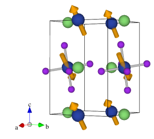
Figure 1: (color online). Magnetic ordering (Type I antiferromagnetic) of the spin-$3/2$ Ru in La₂LiRuO₆ (blue, with arrows).battleLaLiRuO Also shown are the non-magnetic Li (light green) atoms, and two of the Ru-O (purple) octahedra, showing the effects of monoclinic distortion.

The role of spin-orbit coupling in the undistorted cubic double perovskites has been carefully considered by Chen et al. for materials of $d^{1}$ electronic configuration.chensoc In this work, we focus on the $4d^{1}$ and $5d^{1}$ monoclinically distorted double perovskites, and consider the quantum pseudo-spin-$1/2$ models that result, as explained in the main body of the paper. We are particularly interested in the case of a local B^′-O $z$-axis compression, where orbital degeneracy is absent. La₂LiMoO₆ is a candidate for such a material, while the otherwise isostructural Sr₂CaReO₆ features instead a $z$-axis expansion of the octahedra. La₂LiMoO₆ shows no magnetic ordering down to 2 K from either heat capacity or neutron diffraction; however, $\mu$SR measurements show evidence of short-range correlations developing below 20 K.aharendperovMo The Curie-Weiss temperature is negative, $\theta_{C}=-45$ K, indicating predominant antiferromagnetic superexchange. In contrast, Sr₂CaReO₆ shows spin-freezing behavior below 14 K.wiebeSrCaReO

In the present work, we use the Sp($N$) generalization of Heisenberg models to describe these systems.sachdevkagome ; readsachdev ; sachdevread This generalization provides a unifying framework to study the effect of spin magnitude, from semiclassical ordering at “large spin” to possible spin liquid phases for “small spin”.

The ability to capture “large-spin” magnetic order may help to describe the higher-spin analogues of $d^{1}$ double perovskites. In particular, the “spin-$3/2$” analogue of La₂LiMoO₆ is the isostructural La₂LiRuO₆, whose $4d^{3}$ configuration occupies all three $t_{2g}$ orbitals. Since the effective magnetic moment is close to the spin-$3/2$-only moment, there is only slight renormalization due to spin-orbit coupling, and intra-orbital Coulomb repulsion is the dominant effect in determining orbital occupancy. We model this material with a spin-$3/2$ Heisenberg model, given the lack of orbital degeneracy, providing a test for Sp($N$)-predicted ordering at spin larger than $1/2$. In fact, La₂LiRuO₆ shows type I antiferromagnetic ordering below 30 K,battleLaLiRuO where spins are aligned on each $x$-$y$ plane but antiparallel on the $x$-$z$ and $y$-$z$ planes, as seen in Figure 1. This is consistent with the results in the semi-classical (“large spin”) limit of our Sp($N$) model. In contrast, an appropriate pseudo-spin-$1/2$ anisotropic Heisenberg model for La₂LiMoO₆ leads to the conclusion that this system must be very close to a spin liquid state. This may be consistent with the absence of magnetic order down to 2 K seen in experiment.aharendperovMo

The rest of the paper is organized as follows. In §II, we discuss the effects of monoclinic distortion and spin-orbit coupling. This leads us to consider two different models, the planar anisotropy and general anisotropy models, each taking the form of a pseudo-spin Heisenberg model. In §III, we solve for the classical spin ordering of both of these models. In §IV, we describe the Sp($N$) generalization of the Heisenberg model and its mean-field treatment. Results of this mean-field treatment are shown in §V for the planar anisotropy model, and in §VI for the general anisotropy model. An extension to finite temperature is discussed in §VII. In §VIII, we summarize our results and discuss extensions of this work.

II Model

In modelling monoclinically distorted double perovskites with $4d$ or $5d$ magnetic ions, there are two important effects of the monoclinic distortion that should be considered in conjunction with spin-orbit coupling. The first effect of monoclinic distortion is local $z$-axis compression or expansion of the B^′-O octahedra, which affects orbital occupation. The second is the change of orbital orientation due to the geometric distortion, which affects overlap integrals and the resultant interactions. We will derive our models by considering the effect of distortion and spin-orbit coupling on the interactions between $t_{2g}$ orbitals.

One motivation for our models comes from a spin-$1/2$ Heisenberg model obtained via spin-dimer calculation for the isostructural monoclinically distorted double perovskites La₂LiMoO₆ and Sr₂CaReO₆.aharendperovMo In this method, the tetragonal compression (or expansion) of these materials was modelled by assuming occupation of only the $d_{xy}$ orbitals (or equal occupation of only the $d_{xz}$ and $d_{yz}$ orbitals). This method is also sensitive to the effect of the geometric changes resulting from the distortion. However, spin-orbit coupling was not considered, so that the assumed orbital occupation will be slightly incorrect. The result is an anisotropic $S=1/2$ Heisenberg model, with estimates for the relative strengths of the couplings, seen in Table 1.

II.1 Interactions

To understand the effects of the monoclinic distortion and spin-orbit coupling, we first look at the interactions between neighboring $t_{2g}$ orbitals in the case of cubic symmetry, as have been considered in detail by Chen et al.chensoc To facilitate this, we show the six nearest-neighbor directions $\mbox{\boldmath$\delta$}_{n}$ for the FCC lattice in Figure 2. Without distortion, the $a$, $b$ and $c$-axes are simply the Cartesian $x$, $y$ and $z$-axes.

Figure 2: Nearest-neighbor lattice vectors $\mbox{\boldmath$\delta$}_{n}$ and associated nearest-neighbor couplings $J_{n}$ for the FCC lattice.

The strongest interaction is antiferromagnetic superexchange, involving sites and orbitals lying in the same plane. For instance, $d_{xy}$ orbitals on neighboring sites along the $x$-$y$ plane will interact antiferromagnetically. Ferromagnetic interactions between sites on a plane will couple orbitals lying on that plane to orbitals lying perpendicular to it.chensoc Along the $x$-$y$ plane, $d_{xy}$ orbitals interact ferromagnetically with neighboring $d_{yz}$ and $d_{xz}$ orbitals. Quadrupole-quadrupole interactions also exist between all $t_{2g}$ orbitals on neighboring sites, due to different orientations of the quadrupole moments of these orbitals.

II.2 Monoclinic Distortion

The first effect of monoclinic distortion is the local $z$-axis distortion of the $B^{\prime}$-O octahedra, a compression for La₂LiMoO₆ and an expansion for Sr₂CaReO₆. This splits the degeneracy of the three $t_{2g}$ orbitals. The $d_{xz}$ and $d_{yz}$ orbitals will remain degenerate, but the $d_{xy}$ orbital will have a lower energy for a compression and a higher energy for an expansion. Consequently, the occupation of the $d_{xy}$ orbital will be favored or disfavored compared to occupation of the other two orbitals. This is taken as a very important effect in the spin-dimer calculation to explain the relative anisotropies of the two materials.aharendperovMo

The second important effect of the monoclinic distortion is a global $c$-axis elongation, and rotation of the B^′-O octahedra, affecting the overlap of the occupied orbitals, which are now tilted out of plane. An example of this, in the case of La₂LiRuO₆, is shown in Figure 1. The $d_{xy}$ orbitals, for instance, are tilted out of the $a$-$b$ plane, and will have some interaction with $d_{xy}$ orbitals on neighboring planes. In this fashion, many new exchange pathways will contribute at the nearest-neighbor level.

These effects generate a significant amount of exchange anisotropy in the spin-dimer calculation.aharendperovMo The relative coupling strengths estimated by spin-dimer calculation for La₂LiMoO₆ and Sr₂CaReO₆ can be seen in Table 1.

Material	$J_{1}$	$J_{2}$	$J_{3}$	$J_{4}$	$J_{5}$	$J_{6}$
La2LiMoO6	0.14	1.0	0.014	0.014	0.00043	0.00043
Sr2CaReO6	0.87	1.0	0.16	0.16	0.25	0.25

Table 1: Relative strengths of Heisenberg couplings, given in Figure 2, from the spin-dimer calculation of Aharen et al.aharendperovMo

Interactions between $x$-$y$ planes in La₂LiMoO₆ are relatively weak, as expected from dominant in-plane $d_{xy}$-$d_{xy}$ antiferromagnetic interaction and $c$-axis elongation. We note that further in-plane anisotropy is significant, due to the strong effect of Mo-O octahedra rotation upon $d_{xy}$ orbital overlap. In Sr₂CaReO₆, intra-plane interactions are still larger than inter-plane interactions, even though the superexchange between $d_{xy}$ orbitals is not present. The only in-plane superexchange processes occur through tilted $d_{xz}$ or $d_{yz}$ orbitals. Nevertheless, the inter-plane interactions are significantly stronger than in La₂LiMoO₆. The length of the unit cell along the $c$ axis is significantly larger than along the $a$ or $b$ axes, which could explain the smaller inter-plane coupling compared to the intra-plane one. For both materials, however, the planar anisotropy of the couplings is clear, and effects of both geometrical distortion and orbital occupation are important.

II.3 Spin-Orbit Coupling

Beyond monoclinic distortion, we now consider spin-orbit coupling, which can be important in the $4d$ and $5d$ magnetic ions commonly seen in the double perovskites. For instance, spin-orbit coupling in octahedrally coordinated Mo⁵⁺ is estimated to be on the order of 0.1 eV.vulfson The effect of spin-orbit coupling on the $t_{2g}$ orbitals of octahedrally coordinated ions is a well-studied problem. When the octahedral crystal field splitting is significantly large compared to the spin-orbit coupling, we may project out the $e_{g}$ states. Upon projection, the $L=2$ orbital angular momentum for the $d$ orbitals looks like a $L=1$ pseudo-angular momentum operator $\mathbf{l}$ up to a sign change, where $\mathbf{L}\to-\mathbf{l}$. This $L_{\textrm{eff}}=1$ pseudo-orbital angular momentum combines with the $S={1}/{2}$ angular momentum of the single electron to create states of effective total angular momentum $J_{\textrm{eff}}=3/2$ and $1/2$. The spin-orbit coupling $\lambda\mathbf{L}\cdot\mathbf{S}$ breaks the degeneracy of these states, where the four $J_{\textrm{eff}}=3/2$ states have an energy $3\lambda/2$ lower than the two $J_{\textrm{eff}}=1/2$ ones. These $J_{\textrm{eff}}=3/2$ states are written in terms of the $t_{2g}$ ones as

$$\left|\frac{3}{2},\frac{3}{2}\right>=\frac{1}{\sqrt{2}}\left(-\left|yz,\uparrow\right>+i\left|xz,\downarrow\right>\right)$$

$$\left|\frac{3}{2},\frac{1}{2}\right>=\frac{1}{\sqrt{6}}\left(-\left|yz,\downarrow\right>+i\left|xz,\downarrow\right>+2\left|xy,\uparrow\right>\right)$$

$$\left|\frac{3}{2},-\frac{1}{2}\right>=\frac{1}{\sqrt{6}}\left(\left|yz,\uparrow\right>+i\left|xz,\uparrow\right>+2\left|xy,\downarrow\right>\right)$$

$$\left|\frac{3}{2},-\frac{3}{2}\right>=\frac{1}{\sqrt{2}}\left(\left|yz,\downarrow\right>+i\left|xz,\uparrow\right>\right).$$ (1)

With a $d^{1}$ configuration, the occupancy of the $d_{xy}$ orbital upon projection to these states is given bychensoc

$$n_{i,xy}=\frac{3}{4}-\frac{1}{3}(j_{i}^{z})^{2}.$$ (2)

The occupation operators for the other $t_{2g}$ orbitals are given by cyclic permutation of the $x,y,z$ indices, and the single-occupancy constraint $n_{i,xy}+n_{i,xz}+n_{i,yz}=1$ is satisfied.

The effect of projection onto this $J_{\textrm{eff}}=3/2$ subspace, due to large spin-orbit coupling, has been considered by Chen et al. for the cubic materials.chensoc The Hamiltonian can be written in terms of the orbitally-resolved spin operators, such as $\mathbf{S}_{i,xy}=\mathbf{S}_{i}n_{i,xy}$. Upon projecting to the $J_{\textrm{eff}}=3/2$ states, these orbitally-resolved spin operators contain terms both linear and cubic in $\mathbf{j}$. The resulting Hamiltonian, containing terms of 4${}^{\textrm{th}}$ and 6${}^{\textrm{th}}$ order in $\mathbf{j}$, leads to interesting multipolar behavior.chensoc

When spin-orbit coupling is much larger than the local $z$-axis crystal field, the $J_{\textrm{eff}}=3/2$ states provide the relevant starting point, rather than the $t_{2g}$ orbitals. However, one can consider the general splitting of $t_{2g}$ orbital degeneracy in the presence of both spin-orbit coupling and the local $z$-axis distortion. We can model each site with a local Hamiltonian $\mathcal{H}_{\mathrm{loc}}=\Delta\left[(l^{z})^{2}-2/3\right]-\lambda\mathbf{l}\cdot\mathbf{S}$, where $\Delta>0$ is the strength of the crystal field splitting due to local $z$-axis compression. The case for a local $z$-axis expansion has been considered by Jackeli and Khaliullin.jackelikhaliullin We proceed in a similar manner, identifying the relevant low-energy eigenstates of $\mathcal{H}_{\mathrm{loc}}$. Diagonalization of $\mathcal{H}_{\mathrm{loc}}$ determines the lowest-energy Kramers pair to be given by

$$\left|\uparrow\right>_{G}=\frac{\sin{(\theta)}}{\sqrt{2}}\left(i\left|yz,\downarrow\right>+\left|xz,\downarrow\right>\right)-i\cos{(\theta)}\left|xy,\uparrow\right>,$$

$$\left|\downarrow\right>_{G}=\frac{\sin{(\theta)}}{\sqrt{2}}\left(-i\left|yz,\uparrow\right>+\left|xz,\uparrow\right>\right)-i\cos{(\theta)}\left|xy,\downarrow\right>,$$

$$\tan{(2\theta)}=2\sqrt{2}\lambda/(\lambda+2\Delta).$$ (3)

The energy difference between the ground and first excited doublets is given by $-\lambda+(\lambda+2\Delta)(1+1/\cos{(2\theta)})/4$, which goes to zero as $\Delta\to 0$, and approaches $\Delta-{\lambda}/{2}$ when $\Delta\gg\lambda$. We consider the case where this separation is large enough to focus on the lowest-energy doublet. This will require the tetragonal crystal field to be significantly larger than the exchange coupling $J$, regardless of the relative strength of spin-orbit coupling. By projecting out the higher-energy states, we obtain a pseudo-spin-1/2 model.

Within this projection, we consider the form of the interactions in an otherwise cubic double perovskite, beginning with the quadrupole-quadrupole interaction. Due to the fixed orbital occupation in (3), this interaction is constant and will not contribute to our models. The orbitally off-diagonal ferromagnetic interactions, of strength $J^{\prime}$, generate pseudo-spin interactions that are both spatially and spin-anisotropic. For our models, we will focus on the antiferromagnetic interactions. Nearest-neighbor interactions along the undistorted $x$-$y$, $x$-$z$ and $y$-$z$ planes are given by

$$\mathcal{H}_{\textrm{AF}}=J\sum_{<ij>\textrm{ in x-y}}\left(\mathbf{S}_{i}\cdot\mathbf{S}_{j}-\frac{1}{4}\right)n_{i,xy}n_{j,xy}$$

$$+(xy\to yz)+(xy\to xz),$$ (4)

where $n_{i,xy}$ is the occupation operator of the $d_{xy}$ orbital at site $i$.chensoc Upon projection to the lowest-energy doublet, we obtain a Heisenberg model in the pseudo-spin-$1/2$ operators $\mathbf{P}_{i}$,

$$\mathcal{H}^{\prime}=N\left(-\frac{J}{4}\right)+\sum_{<ij>\textrm{ in x-y}}\cos{(\theta)}^{4}J\mathbf{P}_{i}\cdot\mathbf{P}_{j}$$

$$+\sum_{<ij>\textrm{ in x-z}}\sin{(\theta)}^{4}\frac{J}{4}\mathbf{P}_{i}\cdot\mathbf{P}_{j}+\sum_{<ij>\textrm{ in y-z}}\sin{(\theta)}^{4}\frac{J}{4}\mathbf{P}_{i}\cdot\mathbf{P}_{j}.$$ (5)

For $\Delta\ll\lambda$, this result reduces to the one obtained by Chen et al. in the easy-plane limit of the cubic perovskite model with $J^{\prime}=0$.chensoc Without an accurate estimate for the strength of Hund’s coupling to Coulomb repulsion, the ratio $J^{\prime}/J$ is difficult to ascertain. However, we note that the easy-plane result of Chen et al. is an antiferromagnetic state for $J^{\prime}<J$.chensoc Consequently, we consider the physical picture of antiferromagnetic interactions, and as a first-order approximation we ignore the ferromagnetic contributions to the Hamiltonian.

We note that the introduction of spin-orbit coupling results in a reduction of the magnetic moment compared to the case of $d_{xy}$ occupation when $\lambda=0$.

II.4 Planar-Anisotropy and General-Anisotropy Models

The first, and simpler, of the two models considered in this paper is concerned primarily with the effects of the tetragonal crystal field splitting. Without spin-orbit coupling, we see easily from (4) that preferential $d_{xy}$ orbital occupation leads to anisotropic interactions that are stronger on the $x$-$y$ planes. In this case, we have a true spin-$1/2$ antiferromagnetic Heisenberg model. However, considering spin-orbit coupling and tetragonal distortion leads to the pseudo-spin-$1/2$ antiferromagnetic Heisenberg model in (5), with a similar form of anisotropy. From this, we are motivated to study the pseudo-spin-$1/2$ antiferromagnetic Heisenberg model where coupling along the $x$-$y$ plane differs from the coupling along the $y$-$z$ and $x$-$z$ planes. The planar anisotropy model is given in terms of pseudo-spin-1/2 operators (henceforth referred to as $\mathbf{S}_{i}$) by

$$\mathcal{H}_{\textrm{PA}}=J_{\textrm{in}}\sum_{<ij>\textrm{ in x-y}}\mathbf{S}_{i}\cdot\mathbf{S}_{j}$$

$$+J_{\textrm{out}}\sum_{<ij>\textrm{ in y-z}}\mathbf{S}_{i}\cdot\mathbf{S}_{j}+J_{\textrm{out}}\sum_{<ij>\textrm{ in x-z}}\mathbf{S}_{i}\cdot\mathbf{S}_{j}.$$ (6)

Both $J_{\textrm{in}}$ and $J_{\textrm{out}}$ are antiferromagnetic, and one can consider this model as a generalization of the antiferromagnetic model in Eq. (5). The ratio $J_{\textrm{out}}/J_{\textrm{in}}$ depends on the strengths of the spin-orbit coupling and tetragonal distortion of the octahedra, seen in $\Delta/\lambda$. In addition, it captures certain geometrical effects of the monoclinic distortion, such as the global $c$-axis elongation, contributing to the particular planar anisotropy in (6).

The other model considered in this paper will include in full the geometrical effects of the monoclinic distortion. This will generate many other anisotropic interactions, breaking the symmetry of the $x$-$y$ plane. Effective pseudo-spin exchange energies will become intrinsically anisotropic, in addition to the effects of orbital occupation. We will model these like the spin-dimer calculation does, with different strengths of the nearest-neighbor couplings shown in Fig. 2. Due to spin-orbit coupling, the particular parameters $J_{n}$ in Table 1 will not be quantitatively correct. Nonetheless, we will consider them as a starting point to understand the effect of further anisotropy in the interactions. Estimates for corrections due to spin-orbit coupling are given in §VI.2. The general anisotropy model is given by

$$\mathcal{H}_{\textrm{GA}}=\sum_{i}\sum_{n}J_{n}\mathbf{S}(\mathbf{r}_{i})\cdot\mathbf{S}({\mathbf{r}_{i}+\mbox{\boldmath$\delta$}_{n}}).$$ (7)

To analyze the model Hamiltonians (6) and (7), we will use the Sp($N$) generalization of the Heisenberg model, which offers several advantages. The first is that the parameter $N$ allows for a controlled expansion, beginning from the saddle-point solution as $N\to\infty$. The second is that quantum fluctuations can be controlled by a parameter $\kappa$ (where $\kappa=2S$ in the SU(2) case) allowing a transition from a classical-spin limit (large $\kappa$) to one dominated by quantum fluctuations (small $\kappa$). This may capture a changing value of (pseudo)-spin. The gapped $Z_{2}$ spin liquid, obtained as a disordered state in the Sp($N$) generalization, is often seen as a potential ground state in many Heisenberg models. wangvishwanath ; moessnersondhifradkin

The Sp($N$) generalization may be capable of naturally capturing the changing behavior with $S$ seen in the family of magnetic materials isostructural to La₂LiMoO₆. The spin-$3/2$ La₂LiRuO₆ is magnetically ordered, while spin-$1/2$ La₂LiMoO₆ shows short-range correlations and suppression of magnetic order. The isostructural spin-1 La₂LiReO₆ is more amenable to a multi-orbital model, and falls outside the scope of these calculations.aharendperovRe

III Classical Ordering

In this section, we solve both planar anisotropy and general anisotropy models in the limit of classical spins. The magnetic ordering patterns and wavevectors are determined by the $O$($N$) model, where we generalize to $N\to\infty$ components of the spin vector, as explained in Appendix A. We will see in §IV.4 that this corresponds also to the classical limit of the Sp($N$) model.

III.1 Planar-Anisotropy Model

In the planar anisotropy model (6), two phases are found with varying $J_{\textrm{out}}/J_{\textrm{in}}$, the ratio of inter-plane to intra-plane interactions. For $J_{\textrm{out}}<J_{\textrm{in}}$, the intra-plane interactions create antiferromagnetic Néel order within each $x$-$y$ plane. For $J_{\textrm{out}}>J_{\textrm{in}}$, the inter-plane interactions create antiferromagnetic order between planes.

For $J_{\textrm{out}}>J_{\textrm{in}}$, the ordering wavevector $\mathbf{q}$ is given by

$$\mathbf{q}=\frac{\pi}{a/2}\left(0,0,1\right)~{}\mathrm{or}~{}\frac{\pi}{a/2}\left(1,1,0\right).$$ (8)

Spins on each $x$-$y$ plane are aligned, while spins on neighboring planes are antiparallel. Néel ordering is found along the $x$-$z$ and $y$-$z$ planes. The antiferromagnetic interactions between $x$-$y$ layers are satisfied, as seen in Figure 3.

Figure 3: View along the $z$-axis of FCC lattice magnetic ordering of the planar anisotropy model for $J_{\textrm{out}}>J_{\textrm{in}}$. The solid lines indicate an $x$-$y$ plane of the FCC lattice, while the dotted lines indicate a neighboring plane. Spins are aligned on each of the $x$-$y$ planes, but Néel ordered along $x$-$z$ or $y$-$z$ planes.

For $J_{\textrm{out}}<J_{\textrm{in}}$, the ordering wavevector $\mathbf{q}$ is

$$\mathbf{q}=\frac{\pi}{a/2}\left(1,0,k_{z}\right),~{}\frac{\pi}{a/2}\left(0,1,k_{z}\right)$$ (9)

for arbitrary $k_{z}$. Each $x$-$y$ plane takes on the Néel order for a square lattice. The degeneracy in $k_{z}$ indicates that spins on neighboring planes may take any relative overall orientation. An example of this ordering, with $k_{z}=0$, is given in Figure 4.

Figure 4: View along the $z$-axis of FCC lattice magnetic ordering of the planar anisotropy model for $J_{\textrm{out}}<J_{\textrm{in}}$ with $k_{z}=0$. The solid lines indicate an $x$-$y$ plane of the FCC lattice, while the dotted line indicates a neighboring plane. There is Néel ordering along each of the $x$-$y$ and $y$-$z$ planes, but ferromagnetic ordering along the $x$-$z$ plane. Also possible is a state where the ferromagnetic ordering is along the $y$-$z$ plane instead.

We will see in §IV.4 that this degeneracy is broken by the introduction of quantum fluctuations, choosing $k_{z}=0$.

Both of these states show Type I antiferromagnetic ordering on the FCC lattice, where ordering is antiferromagnetic on two of the $x$-$y$, $x$-$z$ or $y$-$z$ planes, and ferromagnetic on the other.

III.2 General Anisotropy Model

The two parameter sets in Table 1 also yield antiferromagnetic ordering in the $x$-$y$ plane, similar to the $J_{\textrm{out}}<J_{\textrm{in}}$ case. However, the degeneracy of $k_{z}$ is broken here at the classical level, where $k_{z}=0$ for both parameter sets. Ordering as in Figure 4 results.

IV Sp($N$) Mean Field Theory

IV.1 Sp($N$) Generalization of the Spin Models

The Sp($N$) method is a large-$N$ generalization of the Schwinger boson spin representation.sachdevkagome ; readsachdev ; sachdevread In the physical case $N=1$, Sp(1) is isomorphic to SU(2), and we have the standard Schwinger boson representation wherein $\mathbf{S}_{ia}=\frac{1}{2}b^{{\dagger}}_{i\alpha}(\mbox{\boldmath$\sigma$}_{a})_{\alpha\beta}b_{i\beta}$ and the boson number per site $b^{{\dagger}}_{i\alpha}b_{i\alpha}\equiv n_{b}=2S$ determines the spin quantum number. Here, $\alpha,\beta=\uparrow,\downarrow$ label the primitive spin-$1/2$ species that comprise the full spin angular momentum. We generalize to $2N$ flavors of bosons, where $\alpha=(m,\sigma)$, labelled by $m=1\ldots N$, and $\sigma=\uparrow,\downarrow$, transforming under the group Sp($N$).sachdevkagome $\kappa=n_{b}/N$ acts in analogous fashion to $2S$ in the SU(2) case, controlling the strength of quantum fluctuations.

When generalized to Sp($N$), the Heisenberg Hamiltonian (7), up to constants involving $n_{b}$, is written as

$$\mathcal{H}=\frac{-1}{2N}\sum_{i}\sum_{n}J_{n}(\mathcal{J}^{\alpha\beta}b^{{\dagger}}_{i\alpha}b^{{\dagger}}_{i+\delta_{n},\beta})(\mathcal{J}_{\gamma\nu}b_{i}^{\gamma}b_{i+\delta_{n}}^{\nu}).$$ (10)

Here, $\mathcal{J}_{\alpha\beta}$ is a $2N\times 2N$ block-diagonal antisymmetric tensor, given by

$$\mathcal{J}_{m\sigma,m^{\prime}\sigma^{\prime}}=\delta_{m,m^{\prime}}\begin{pmatrix}0&1\\ -1&0\end{pmatrix}.$$ (11)

IV.2 Mean-Field States

The quartic terms in (10) can be quadratically decoupled by the mean field

$$Q_{in}=\frac{1}{N}\left<\sum_{m}\varepsilon_{\sigma\sigma^{\prime}}b^{{\dagger}}_{im\sigma}b^{{\dagger}}_{i+\delta_{n},m\sigma^{\prime}}\right>.$$ (12)

When the boson dispersion becomes gapless, we allow for a condensate, $b_{i1\sigma}=\sqrt{N}x_{i\sigma}\in\mathbb{C}$, where $\sigma=\uparrow,\downarrow$, so that $\langle b_{i1\sigma}\rangle$ has a finite expectation value. This will account for the appearance of long-range magnetic order.

The projective symmetric group analysis may be used to characterize possible mean-field ground states; for Sp($N$) this has been applied to many other Heisenberg models.wangvishwanath Qualitatively different states are distinguished by the value of a flux quantity for plaquettes of the lattice. The flux on a plaquette of sites $a\ldots z$ is defined by the phase $\Phi$ intchernyshyovflux

$$|\Xi|e^{i\Phi}=\sum_{a\ldots z}Q_{ab}(-Q_{bc}^{*})\ldots Q_{yz}(-Q_{za}^{*}).$$ (13)

A nearest-neighbor Heisenberg model will favor the zero-flux states at small $\kappa$, particularly for plaquettes of smaller length.tchernyshyovflux On the bipartite cubic lattice, for instance, a translationally invariant choice of $Q_{ij}$ yields zero flux on any plaquette. Since the FCC lattice is frustrated, a translationally invariant $Q_{ij}=-Q_{ji}$, while giving zero flux on most plaquettes, leaves $\pi$ flux on a small number of plaquettes. In particular, assuming all $Q$ to be translationally invariant and positive, the four-site plaquettes with $\pi$ flux have sites on both the $x$-$y$ and $y$-$z$ planes, such as $\mathbf{i},\mathbf{i}+\mbox{\boldmath$\delta$}_{1},\mathbf{i}+\hat{y},\mathbf{i}+\mbox{\boldmath$\delta$}_{3}$, where $\mathbf{i}$ and $\mathbf{i}\pm\hat{y}$ are joined by the plaquette. There are eight such plaquettes with $\pi$ flux, of a total of thirty-six four-site plaquettes involving site $\mathbf{i}$. This provides motivation to consider translationally invariant mean-field solutions, which we restrict ourselves to in this work.

IV.3 Mean-Field Hamiltonian

After decoupling in the site-independent $Q_{n}$ fields, the Hamiltonian (10) becomes

$$\mathcal{H}=\sum_{i,n}J_{n}\left[-\frac{Q_{n}}{2}\varepsilon_{\sigma\sigma^{\prime}}\left(\sum_{\tilde{m}=2}^{N}b_{i}^{\tilde{m}\sigma}b_{i+\delta_{n}}^{\tilde{m}\sigma^{\prime}}+x_{i}^{\sigma}x_{i+\delta_{n}}^{\sigma^{\prime}}N\right)\right.$$

$$\left.+h.c.+\frac{N}{2}\left|Q_{n}\right|^{2}\right]+$$

$$\sum_{i}\mu_{i}\left(-n_{b}+\sum_{\tilde{m}=2}^{N}b^{{\dagger}}_{i\tilde{m}\sigma}b_{i}^{\tilde{m}\sigma}+N{x}^{*}_{i\sigma}x_{i}^{\sigma}\right).$$ (14)

Here, the boson number constraint is enforced on average by the inclusion of the Lagrange multiplier $\mu_{i}$. We assume tranlsational invariance, with $\mu_{i}=\mu$. We have allowed the $m=1$ component to condense, represented by $x_{i}^{\sigma}\in\mathds{C}$.

The saddle-point Hamiltonian (for $N\to\infty$) is derived in full in Appendix B. The first step is a Fourier transform defined by $b_{i}=\frac{1}{\sqrt{N_{s}}}\sum_{k}b_{k}e^{-ik\cdot r_{i}}$. The second step is a Bogoliubov transformation diagonalizing the Hamiltonian, yielding a quasiparticle energy $\omega_{k}=\sqrt{\mu^{2}-(\sum_{n}J_{n}Q_{n}\sin{(k\cdot\delta_{n})})^{2}}$. The transformation is defined by $\mathbf{b}=T^{-1}\mbox{\boldmath$\gamma$}$, where the Hamiltonian is diagonal in the $\gamma$ basis. The condensate enters only via the total density $n=\sum_{k\sigma}|x_{\mathbf{k}}^{\sigma}|^{2}$, and $\pm\mathbf{k}_{1}$, the wavevectors of the boson dispersion minimum where the condensate forms.

We then write the diagonalized Hamiltonian as

$$\frac{\mathcal{H}}{N_{s}N}=\sum_{\delta}\frac{J_{\delta}}{2}|Q_{\delta}|^{2}+\mu\left(-1-\kappa+n\right)$$

$$+n\sum_{\delta}J_{\delta}Q_{\delta}\sin{(k_{1}\cdot\delta)}$$

$$+\frac{1}{N_{s}}\sum_{k}\omega_{k}\left(1+\gamma^{{\dagger}}_{k\uparrow}\gamma_{k\uparrow}+\gamma^{{\dagger}}_{k\downarrow}\gamma_{k\downarrow}\right).$$ (15)

IV.4 Semiclassical Large-$\kappa$ Limit

We take advantage of the Sp($N$) fluctuation parameter $\kappa$ to look at the semiclassical magnetic order from the $\kappa\to\infty$ limit. This provides a link from the classical order of §III to the magnetic order seen at finite $\kappa$.

We begin by approximating the Hamiltonian for $\kappa\gg 1$. Here, leading-order behavior in the Hamiltonian is of O($\kappa^{2}$). Corrections, of O($\kappa$), act to split degeneracy of the classical ordering.sachdevkagome We have that $Q$, $\mu$ and $n$ are all O($\kappa$) as $\kappa\gg 1$. $E_{C}$, the largest contribution to the energy is of O($\kappa^{2}$):

$$\frac{E_{C}}{N_{s}N}=\sum_{\delta}\frac{J_{\delta}}{2}|Q_{\delta}|^{2}+\mu\left(-\kappa+n\right)$$

$$+n\sum_{\delta}J_{\delta}Q_{\delta}\sin{(k_{1}\cdot\delta)},$$ (16)

while the first-order quantum correction $E_{1}$, of O($\kappa$), is given by

$$\frac{E_{1}}{N_{s}N}=-\mu+\frac{1}{N_{s}}\sum_{k}\omega_{k},$$ (17)

where $Q$, $\mu$ and $n$ are given by solutions minimizing the classical energy (16).sachdevkagome The mean-field equations for $E_{C}$ are easily solved, yielding $n=\kappa$, $\mu=-\sum_{n}J_{n}Q_{n}\sin{(k_{1}\cdot\delta_{n})}$, and $Q_{m}=-\kappa\sin{(k_{1}\cdot\delta_{m})}$. We can then write $E_{C}$ as a function of the minimum wavevector $\mathbf{k}_{1}$:

$$\frac{E_{C}}{N_{s}N}=-\kappa^{2}\sum_{n}\frac{J_{n}}{2}\sin^{2}{(\mathbf{k}_{1}\cdot\mbox{\boldmath$\delta$}_{n})}.$$ (18)

With the boson dispersion minimum at $\pm\mathbf{k}_{1}$, spin ordering occurs at the wavevectors $\mathbf{q}=\pm 2\mathbf{k}_{1}$. The minimum of $E_{C}$ corresponds to an ordering pattern equivalent to that of the classical $O$($N$) model (see Appendix A for details).garanincanalspyrochlore The correction (17) can then easily be computed for all $\mathbf{k}_{1}$ (with corresponding $Q$, $\mu$, $n$) in the degenerate set of minima of (18).

V Planar Anisotropy Model Results

In this section we study the planar anisotropy model with in-plane coupling $J_{\textrm{in}}$ ($J_{1}=J_{2}$) and out-of-plane coupling $J_{\textrm{out}}$ ($J_{3}=J_{4}=J_{5}=J_{6}$). We study the effect of quantum fluctuations, controlled by $\kappa$, and coupling anisotropy, controlled by $J_{\textrm{out}}/J_{\textrm{in}}$. In §III, we saw classical Néel ordering on each $x$-$y$ plane. The first-order quantum correction $E_{1}$ in (17) breaks the degeneracy. After this “order by disorder”, the ordering wavevectors are

$$\mathbf{q}=\frac{\pi}{a/2}\left(1,0,0\right)~{}\mathrm{or}~{}\frac{\pi}{a/2}\left(0,1,1\right),$$

$$\mathbf{q}=\frac{\pi}{a/2}\left(0,1,0\right)~{}\mathrm{or}~{}\frac{\pi}{a/2}\left(1,0,1\right).$$ (19)

Spins are aligned along either the $x$-$z$ or $y$-$z$ planes. Ordering along one such direction was seen in Figure 4.

As $\kappa$ is reduced from this limit, we wish to see the evolution of the ordering wavevector and mean-field parameters. For small $\kappa$, we investigate the destruction of the ordered state by quantum fluctuations. We note that the semiclassical solutions, for all values of $J_{\textrm{out}}/J_{\textrm{in}}$, all feature $|Q_{1}|=|Q_{2}|,|Q_{3}|=|Q_{4}|,$ and $|Q_{5}|=|Q_{6}|$. Motivated additionally by the equality of in-plane couplings, $J_{1}=J_{2}$, and of between-plane couplings, $J_{4}=J_{4}=J_{5}=J_{6}$, we take an ansatz with $Q_{1}=Q_{2},Q_{3}=Q_{4},$ and $Q_{5}=Q_{6}$. The relative signs, such as between $Q_{1}$ and $Q_{2}$, correspond to making a particular gauge choice. With such an ansatz, the semiclassical solutions remain unchanged, with wavevectors (8) or (19) as appropriate. Furthermore, relaxing the ansatz suggests that the equivalence $|Q_{1}|=|Q_{2}|,|Q_{3}|=|Q_{4}|,$ and $|Q_{5}|=|Q_{6}|$ is retained down to low $\kappa$. With this ansatz, we numerically solve the mean-field equations, given explicitly in Appendix B. The resulting phase diagram is given in Fig. 5, in which there are five phases to consider.

Figure 5: Heuristic phase diagram for the $Q_{1},Q_{3},Q_{5}$ ansatz of the planar anisotropy model. Note that the label $Q_{m}=0$ indicates that $Q_{m}$ is negligibly small (compared to $\kappa$ and the finite $Q$) in the condensed phase; $Q_{m}$ is identically zero in the corresponding spin liquid phases. Solid lines indicate second-order transitions, while dashed lines indicate first-order transitions.

V.1 Inter-plane Antiferromagnetic Order

This state is an extension of the classically ordered state for $J_{\textrm{out}}>J_{\textrm{in}}$, with antiparallel magnetization on neighboring $x$-$y$ planes. Ferromagnetic ordering is seen along the $x$-$y$ plane, with Néel ordering along the $x$-$z$ and $y$-$z$ planes. In this state, the intra-plane $Q_{1}=Q_{2}$ is significantly smaller than the intra-plane $Q_{3}$ through $Q_{6}$. The ordering wavevector has only small corrections to the classical result (8).

V.2 $x$-$y$ Plane Néel Order

This state is an extension of the classically ordered state for $J_{\textrm{out}}<J_{\textrm{in}}$, with Néel order on the $x$-$y$ planes. It is characterized by large $|Q_{1}|=|Q_{2}|$ within the $x$-$y$ plane. Of the two independent inter-plane $Q$, one is significantly smaller than the other, depending on the gauge choice of ferromagnetic order direction (along the $x$-$z$ or $y$-$z$ plane). The ordering wavevector has only small corrections to the semiclassical result (19).

V.3 Inter-Plane Spin Liquid

This state is a disordered analogue of the inter-plane ordered state (§V.1) for $J_{\textrm{out}}>J_{\textrm{in}}$. However, the intra-plane $Q_{1}=Q_{2}$ are identically zero in this state. While the direct intra-plane correlations are consequently zero, the finite inter-plane $Q$ prevent the lattice from decoupling. The minimum wavevector, determining short-range order, still has only small corrections compared to the ordered minimum (8). The transition into this state from the intra-plane ordered state, as $\kappa$ is lowered, is second-order.

V.4 Three-Dimensional Intra-Plane Spin Liquid

This state is a disordered analogue of the inter-plane ordered state (§V.2) for $J_{\textrm{out}}<J_{\textrm{in}}$. However, one of the intra-plane $Q$ is now identically zero, such as $Q_{3}=Q_{4}$. The other intra-plane $Q$ is nonzero, but still smaller than the in-plane $Q_{1}=Q_{2}$, preventing the lattice from decoupling. As before, the minimum wavevector, determining short-range order, has only small corrections compared to the ordered minimum (19). The transition into this state from the intra-plane ordered state, as $\kappa$ is lowered, is second-order.

V.5 Quasi-Two-Dimensional Spin Liquid

In this state, all inter-plane $Q$ vanish: $Q_{3}=Q_{4}=Q_{5}=Q_{6}=0$. The system then consists of decoupled two-dimensional $x$-$y$ planes in this mean-field theory. The transitions into this state, from either the ordered or disordered intra-plane states for $J_{\textrm{out}}<J_{\textrm{in}}$, are weakly first-order. The minimum (short-range order) wavevector no longer takes the semiclassical value, instead taking a different value among the classical solutions (9), with $k_{z}\sim 0.15$.

V.6 Tricritical Point and Destruction of Order

We find a tricritical point at $\tilde{J}_{\textrm{out}}=0.58J_{\textrm{in}}$ separating the intra-plane spin-liquid phases from the $x$-$y$ plane Néel ordered phase. For $J_{\textrm{in}}>J_{\textrm{out}}>\tilde{J}_{\textrm{out}}$, the ordered state first enters the three-dimensional spin-liquid state as $\kappa$ is decreased. A first-order transition to the two-dimensional spin liquid follows as $\kappa$ decreases further. The $\kappa$ range of this three-dimensional spin liquid narrows as $J_{\textrm{out}}$ reaches tricritical point, as seen in Figure 5. For $J_{\textrm{out}}<\tilde{J}_{\textrm{out}}$, in-plane coupling pushes the system to decouple. However, we expect that the $Q=0$ decoupling seen in all three mean-field spin liquid states is an artifact of the mean-field theory, and that $1/N$ corrections will restore a small yet non-zero value to these $Q$.

The critical $\kappa$ value of the destruction of magnetic ordering, $\kappa_{c}$, is fairly small in this planar anisotropy model. $\kappa_{c}$ ranges from $0.1$ for large $J_{\textrm{out}}$ to 0.4 for small $J_{\textrm{out}}$. In the physical $N=1$ case, $\kappa=1$ corresponds to the “most quantum” limit of $S=1/2$. Our $N\to\infty$ solution indicates that ordering is likely to occur, even though mean-field theory overestimates ordering. While $\kappa_{c}$ will differ in the exact $N=1$ theory, the values of $\kappa_{c}\sim 0.1-0.4$ are too small to account for the behavior of La₂LiMoO₆.

VI General Anisotropy Model Results

VI.1 Spin Dimer Parameters

We now turn to the particular parameter set in Table 1 modelling La₂LiMoO₆. We saw that the semi-classical limit led to Type I antiferromagnetic order, with Néel order on the $x$-$y$ planes. As for the planar-anisotropy model, we take advantage of coupling symmetry to simplify the mean-field calculation. We make the ansatz $Q_{3}=Q_{4}$ and $Q_{5}=Q_{6}$, since $J_{3}=J_{4}$ and $J_{5}=J_{6}$. The semiclassical result satisfies this, while relaxing the ansatz again suggests this structure carries to low $\kappa$. Then we numerically solve the resulting mean-field equations. The mean-field solution finds that ordering persists down to $\kappa_{c}=0.986$. As in the planar anisotropy case, the ordering wavevector changes little with $\kappa$, and $Q_{5}$ remains significantly smaller than the other $Q$. At $\kappa_{c}$, there is a weakly first-order phase transition into a disordered state with $Q_{1}=Q_{3}=Q_{5}=0$. This highly anisotropic mean-field solution consists of decoupled quasi-one-dimensional chains, with $Q_{2}$ contributing the only non-zero correlation. The phase diagram for the general anisotropy model with parameters modelling La₂LiMoO₆ is given in Figure 6. As before, we expect $1/N$ corrections to remove this decoupling.

Figure 6: Phase diagram as a function of $\kappa$ for the general anisotropy model with parameters for La₂LiMoO₆, from Table 1. For $\kappa$ larger than $\kappa_{c}=0.986$, the system is in a three-dimensional magnetically ordered state, as in the semiclassical limit. For $\kappa$ smaller than $\kappa_{c}$, the system is in an anisotropic and highly decoupled spin liquid state.

The parameter set for Sr₂CaReO₆ in Table 1 behaves similarly, although the transition occurs at a smaller $\kappa_{c}\cong 0.41$, similar to the values from the planar anisotropy model.

Two comparisons to the planar anisotropy model are relevant. The first is that at large exchange anisotropy, the mean-field theory continues to predict immediate transitions from magnetic order into maximally decoupled spin liquid states. Additionally, this anisotropy stabilizes these decoupled states. For the La₂LiMoO₆ parameters, we see a marked increase in $\kappa_{c}$, which falls quite close to 1. This saddle-point solution suggests that the $S=1/2$ system must be very close to the transition to a spin-liquid state, even if magnetic order eventually appears at very low temperature. The effect of further quantum or thermal fluctuations may be sufficient to destroy the order. This could explain why no long-range order is observed in La₂LiMoO₆ down to 2 K, while $\mu$SR shows at most short-ranged order. The distortion of La₂LiMoO₆ from the cubic perovskite structure is key in moving beyond the magnetic order predicted by the planar anisotropy model.

VI.2 Corrections to In-Plane and Out-of-Plane Anisotropy

While the Table 1 parameters give a good picture of the anisotropy of La₂LiMoO₆, they will not be quantitatively correct. We wish to look at deviations due to the inclusion of spin-orbit coupling, from the viewpoint of in-plane and out-of-plane anistropy. The change in orbital occupation will result in a reduction of $d_{xy}$-mediated coupling as spin-orbit coupling increases, along with new contributions, primarily out-of-plane, from $d_{xz}$ and $d_{yz}$ occupation. From these considerations, we estimate changes to $J_{n}$ so as to minimize the resulting anisotropy, thus estimating a lower bound for $\kappa_{c}$ upon inclusion of spin-orbit coupling. We determine the effective couplings $J_{n}$ in a manner similar to model (5), but with intrinsically anisotropic exchange modified by orbital occupation. In general, we have

$$J_{n}\to\cos{(\theta)}^{4}J_{n}^{xy}+\frac{1}{4}\sin{(\theta)}^{4}J_{n}^{xz,yz},$$ (20)

with $\theta$ as defined in (3). While the $\theta=0$ spin-dimer parameters give $J_{n}^{xy}$, the $J_{n}^{xz,yz}$ are unknown. Since they arise from octahedral tilting, the in-plane $J_{n}^{xz,yz}$ will be quite small, similar to how the out-of-plane $J_{n}^{xy}$ are small. Since $0.25\sin{(\theta)}^{4}$ is also small, we ignore that term by estimating $J_{1,2}^{xy}=0$. For the out-of-plane interactions, we will make a large estimate for $J_{n}^{xz,yz}$ to minimize the out-of-plane anisotropy, by taking $J_{3,4,5,6}^{xz,yz}=J_{2}^{xy}$, the largest exchange scale in the problem. In terms of the spin-dimer parameters $J_{n}^{SD}$, we estimate the change in magnitude of $J_{n}$ due to the change in orbital occupation from spin-orbit coupling by taking

$$J_{1,2}=\cos{(\theta)}^{4}J_{1,2}^{SD},$$

$$J_{3,4,5,6}=\cos{(\theta)}^{4}J_{3,4,5,6}^{SD}+\frac{1}{4}\sin{(\theta)}^{4}J_{2}^{SD}.$$ (21)

For the case of $\lambda\gg\Delta$, we find that $\kappa_{c}$ reduces to $0.86$. However, for a moderate case of $\lambda=\Delta$, we find that there is only a slight reduction in $\kappa_{c}$ to $0.98$. For moderate values of $\lambda/\Delta$, these mean-field results indicate that the system is still close to a disordered state; however, this will be sensitive to the value of $\lambda/\Delta$.

Exchange anisotropy has shown to be very important, from the results for the spin-dimer parameters and the spin orbit coupling rescaled values (21). To better understand the combined effect of in-plane and out-of-plane anisotropy, we consider a model with slightly less than the full anisotropy, where $J_{1}=R_{I}J_{2}$, $J_{3}=J_{4}=R_{O}J_{2}$, and $J_{5}=J_{6}=R_{O}R_{I}J_{2}$. This captures the in-plane ($R_{I}$) and out-of-plane ($R_{O}$) anisotropy, differing from the full anisotropy only in the very small exchange parameters $J_{5}$ and $J_{6}$. In Figure 7 we show $\kappa_{c}$ as a function of $R_{O}$, for several values of $R_{I}$. We see that $\kappa_{c}$ decreases fairly evenly as either $R_{O}$ or $R_{I}$ increases.

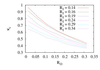
Figure 7: (color online). Critical value $\kappa_{c}$ of destruction of magnetic order. Two types of anisotropy are considered. $R_{I}$ is the ratio of the anisotropy within $x$-$y$ planes, while $R_{O}$ is the ratio of anisotropy between these planes.

This confirms that both in-plane and out-of-plane anisotropy are important in securing a large $\kappa_{c}$.

VII Finite Temperature

Thermal fluctuations of the quasiparticles in (15) introduce, beyond quantum fluctuations, another mechanism inducing disorder. At nonzero temperatures, these excitations have a thermal Bose distribution. The energy $\left<\mathcal{H}\right>$ and the mean-field equations, (15) and (31), are modified accordingly. Thermal fluctuations will reduce magnetic ordering and correlations. We see different finite temperature behavior depending on the state (ordered or spin liquid) seen at $T=0$ for a given set of $J_{n}$ and $\kappa$.

VII.1 Zero-Temperature Disordered Phases

From disordered phases, as $T$ increases, the magnitudes of all $Q$ decrease. The smaller the value of $Q$ at $T=0$, the lower the temperature at which $Q$ reaches zero. At a large enough temperature, all $Q$ are zero, describing a perfectly paramagnetic state, where spins are independent and completely uncorrelated. This unphysical behavior at high temperature is typical of $N\to\infty$ solutions of Schwinger boson mean-field theories, and disappears for smaller values of $N$.tchernyshyovsondhi

VII.2 Zero-Temperature Magnetic Phases

From ordered phases, as $T$ increases, the condensate density $n$ decreases along with the mean-field parameters $|Q_{n}|$. It similarly reaches zero at a large enough $T$. At large $\kappa$, the transition to the perfect paramagnet state is first-order, with the system remaining in the ordered state until all $Q$ and $n$ discontinuously jump to zero. This occurs even for moderate values of $\kappa$, such as $\kappa\sim 0.5$ in the planar anisotropy model. For instance, with $J_{\textrm{out}}=0.54J_{\textrm{in}}$ and $\kappa=0.5$, this transition occurs at $T=0.44J_{\textrm{in}}$. With $\theta_{C}=-45$ K and $S={1}/{2}$, the transition temperature $T=53$ K, an overestimate to be expected of mean-field theory.

For smaller $\kappa$, close to the disordered state boundary, the transition is second order. Furthermore, the order can be destroyed before the $Q$ become zero; the system has a second-order transition to a thermally disordered state before entering the perfect paramagnet state. We show such an example in Figure 8. Here, $\kappa=0.2$, just above the zero-temperature critical $\kappa_{c}$ for $J_{\textrm{out}}=0.54J_{\textrm{in}}$. At $T=0$, the transition with varying $\kappa$ went from ordered state directly into a quasi-two dimensional spin liquid.

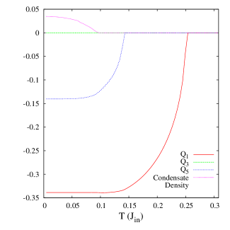
Figure 8: (color online). Mean field and condensate density (magenta) destruction with increasing temperature, shown for $J_{\textrm{out}}=0.54J_{\textrm{in}}$ and $\kappa=0.2$ in the planar anisotropy model. Above $T\sim 0.1J_{\textrm{in}}$, the magnetic ordering is destroyed, leaving a thermally disordered state. As $Q_{5}$ (blue) and $Q_{1}$ (red) become zero, the system enters a two-dimensionally or completely decoupled state, respectively.

At finite temperature, we see that there is a window, $0.1J_{\textrm{in}}\lesssim T\lesssim 0.15J_{\textrm{in}}$, where a three-dimensional disordered state exists, in contrast with the decoupling behavior of the $T=0$ mean-field theory.

The general anisotropy model with La₂LiMoO₆ parameters shows similar behavior. However, at $\kappa=1$, the transition from the ordered state looks weakly first-order, with the system directly entering a quasi-two-dimensional decoupled state where only $Q_{1}$ and $Q_{2}$, both in the $x$-$y$ plane, are nonzero. A fully three-dimensional disordered state is not predicted here by the finite-temperature mean-field theory. Nonetheless, this case illustrates how fluctuations destroy magnetic order and inhibit coupling in the spin-liquid states. As before, we expect $1/N$ corrections to further restore correlations.

VII.3 Heat Capacity

The presence of the perfect paramagnet state is an artifact of the mean-field theory. Regardless, the magnetic contribution to the heat capacity is an important physical quantity, and can be reliably calculated in this approach at low temperatures. $C_{V}$ is found straightforwardly from $d{\left<\mathcal{H}\right>}/d{T}$. In the magnetically ordered states, we find that $C_{V}\propto T^{3}$ at low temperatures. This is expected from three-dimensional antiferromagnetic spin wave contributions. In the disordered states, $C_{V}\propto\exp{(-\Delta_{G}/k_{B}T})$. $\Delta_{G}$ scales roughly with the spin gap, as expected for gapped states. Unfortunately, the lattice match material for La₂LiMo₆ was not useful in subtracting the lattice contribution to the heat capacity.aharendperovMo Without clear data for the magnetic contribution to the specific heat, direct comparison is not feasible. For a system close to the ordering transition, such as the general anisotropy model for La₂LiMoO₆, the $T^{3}$ behavior persists only at extremely low temperatures, further complicating potential comparison.

VIII Conclusion

We have modelled the effects of monoclinic distortion and spin-orbit coupling in $4d^{1}$ or $5d^{1}$ double perovskites. Local $z$-axis distortion of the magnetic ion-oxygen octahedra changed $d_{xy}$ orbital occupation compared to the other $t_{2g}$ orbitals. Geometrical effects of monoclinic distortion changed orbital overlaps, introduced multiple exchange pathways and generated significant anisotropy. Considering spin-orbit coupling in conjunction with the local $z$-axis crystal field yielded a lowest-energy doublet of states and a pseudo-spin-$1/2$ Heisenberg model from antiferromagnetic interactions. We considered first the general case where interactions between sites on $x$-$y$ planes differ in strength from interactions between these planes. This planar anisotropy model was studied for a general ratio of these two couplings. Geometrical changes of the monoclinic distortion induce further anisotropy among the interactions, especially within the $x$-$y$ plane, leading to the general anisotropy model, studied for particular parameters modelling La₂LiMoO₆, estimated from spin-dimer calculation. aharendperovMo We solved both these models in the saddle-point limit of the Sp($N$) generalization of the Heisenberg model. Semi-classical ordering was determined to be Type I antiferromagnetic, with antiferromagnetic order on two of the $x$-$y$, $x$-$z$, $y$-$z$ planes, and ferromagnetic order on the other. The Sp($N$) method connected the semiclassical results to the limit of large quantum fluctuations. The large interaction anisotropy of the general anisotropy model predicted disordering at a relatively large $\kappa_{c}=0.986$. The $N=1$ pseudo-spin $1/2$ system was determined to be very close to a disordered state, even if order sets in at a low temperature. This could explain the lack of long-range order seen down to 2 K in La₂LiMoO₆. Furthermore, estimates of the effect of spin-orbit coupling on the spin-dimer calculation parameters of Table 1 reduced $\kappa_{c}$ only to $0.98$ for moderate strength of spin-orbit coupling. The system is still close to a disordered state in this case.

Further experimental and theoretical inquiries follow as natural extensions of our investigation. Single-crystal experimental results would be useful, primarily in determining the short-range ordering wavevector of La₂LiMoO₆. Results at temperatures lower than 2 K could determine specifically how antiferromagnetic order is being suppressed. Finally, estimates of the strength of the spin-orbit coupling and crystal field splitting would guide a more precise model of the monoclinic distortion.

Appendix A Classical $O$($N$) Model

We begin by writing the real-space partition function for the Heisenberg Hamiltonian on the FCC lattice,

$$Z=\int D\phi D\mu\exp{(-S(\phi,\mu))},~{}\textrm{where }S(\phi,\mu)=$$

$$\beta\sum_{ij}\left[\frac{J_{ij}}{2}\mbox{\boldmath$\phi$}_{i}\cdot\mbox{\boldmath$\phi$}_{j}+\frac{\mu_{i}}{2}\delta_{ij}(\mbox{\boldmath$\phi$}_{i}\cdot\mbox{\boldmath$\phi$}_{i}-N)\right].$$ (22)

Here, the $O$($N$) model generalizes the spin $\phi$ from a three-component vector to an N-component vector. The first step is to take the Fourier transform defined by $\mbox{\boldmath$\phi$}_{i}=\frac{1}{\sqrt{N_{s}}}\sum_{\mathbf{k}}\mbox{\boldmath$\phi$}_{\mathbf{k}}\exp{(-i\mathbf{k}\cdot\mathbf{r}_{i})},$ where $N_{s}$ is the number of sites of the lattice. After the Fourier transform, we have

$$\frac{S}{\beta N_{s}N}=-\frac{\mu}{2}+\frac{1}{N_{s}}\sum_{\mathbf{k}}|\phi_{\mathbf{k}}|^{2}$$

$$\times\left(\frac{\mu}{2}+\sum_{n=1}^{6}J_{\delta_{n}}\cos{(\mathbf{k}\cdot\mbox{\boldmath$\delta$}_{n})}\right)$$ (23)

$$Z\propto\int d\mu\prod_{\mathbf{k}}d\phi_{\mathbf{k}}d\phi_{\mathbf{k}}^{*}\exp{(-S)}.$$ (24)

We perform the Gaussian integral over $\phi_{\mathbf{k}}$ and $\phi_{\mathbf{k}}^{*}$, giving

$$Z\propto\int d\mu\exp{\left(\frac{\beta\mu}{2}N_{s}N-\sum_{\mathbf{k}}\ln{\left(\frac{D(k,\mu)N\beta}{\pi}\right)}\right)},$$

$$D(k,\mu)=\frac{\mu}{2}+\sum_{n=1}^{6}J_{n}\cos{(\mathbf{k}\cdot\mbox{\boldmath$\delta$}_{n})}.$$ (25)

The corresponding saddle-point solution gives $\mu$ from

$$1=\frac{1}{N_{s}}\sum_{\mathbf{k}}\frac{1}{N\beta D(k,\mu)}.$$ (26)

The spin-spin correlation function scales as

$$\left<\mbox{\boldmath$\phi$}_{\mathbf{k}}\cdot\mbox{\boldmath$\phi$}_{\mathbf{k}^{\prime}}\right>\propto\delta_{\mathbf{k}^{\prime},-\mathbf{k}}\frac{1}{\beta D(k,\mu)}.$$ (27)

As $\beta\to\infty$, the minimum of $D(\mathbf{k},\mu)$ will become the dominant contribution; magnetic ordering will occur with the wavevector $\mathbf{q}$ that minimizes $\sum_{n=1}^{6}J_{n}\cos{(\mathbf{q}\cdot\mbox{\boldmath$\delta$}_{n})}$.

Appendix B Saddle-Point Solution

To find the saddle-point solution, we first look at the Fourier transform, defined as $b_{i}=\frac{1}{\sqrt{N_{s}}}\sum_{k}b_{k}e^{-ik\cdot r_{i}}$. After taking this transform, the Hamiltonian (14) becomes

$$\frac{\mathcal{H}}{N_{s}N}=\sum_{n}\frac{J_{\delta_{n}}}{2}|Q_{\delta_{n}}|^{2}+\mu\left(-1-\kappa+\frac{1}{N_{s}}\sum_{k}x_{k\sigma}^{*}x_{k}^{\sigma}\right)$$

$$+\frac{1}{N_{s}}\sum_{kn}\left(\frac{-J_{\delta_{n}}Q_{\delta_{n}}}{2}\varepsilon_{\sigma\sigma^{\prime}}x_{k}^{\sigma}x_{-k}^{\sigma^{\prime}}e^{ik\cdot\delta}+h.c.\right)$$

$$+\frac{1}{N_{s}N}\sum_{mk}\begin{pmatrix}b^{{\dagger}}_{km\uparrow}&&b_{-km\downarrow}\end{pmatrix}\begin{pmatrix}\mu&&B_{k}\\ -B_{k}&&\mu\end{pmatrix}\begin{pmatrix}b_{km\uparrow}\\ b^{{\dagger}}_{-km\downarrow}\end{pmatrix};$$

$$B_{k}=i\sum_{n}J_{\delta_{n}}Q_{\delta_{n}}\sin{(k\cdot\delta_{n})}$$ (28)

where $N_{s}$ is the number of sites in the system.

The quadratic part of the mean-field Hamiltonian in (28) is diagonalized by a standard Bogoliubov transformation.blaizotripka With the quasiparticle energy $\omega_{k}=\sqrt{\mu^{2}-(\sum_{n}J_{n}Q_{n}\sin{(k\cdot\delta_{n})})^{2}}$, the diagonalized quadratic terms are

$$\frac{1}{N_{s}}\sum_{k}\omega_{k}\left(1+\gamma^{{\dagger}}_{k\uparrow}\gamma_{k\uparrow}+\gamma^{{\dagger}}_{k\downarrow}\gamma_{k\downarrow}\right).$$ (29)

Here, the transformation is defined by $\mathbf{b}=T^{-1}\mbox{\boldmath$\gamma$}$, where the columns of $T^{-1}$ are the eigenvectors of ${\eta}M$, $M$ is the quadratic Hamiltonian matrix in (28), and the $2N\times 2N$ ${\eta}$ is given by

$$\eta_{\alpha\beta}=\begin{cases}\delta_{\alpha\beta}&\alpha\leq N\\ -\delta_{\alpha\beta}&\alpha>N\end{cases}.$$

The structure of the condensate can be determined from the associated mean-field equation: $\partial{\left<\mathcal{H}\right>}/\partial{x^{\sigma}_{k}}=0.$ The solution to the disordered case ($x=0$) has a gapped dispersion. We can track when the gap vanishes and bosons begin to condense. We find that $x_{k}^{\uparrow}$ is a linear combination of condensates at the minimum wavevectors $\pm\mathbf{k}_{1}$: $x_{k}^{\uparrow}=c_{1}\delta_{k-k_{1}}+c_{2}\delta_{k+k_{1}}$. We then rewrite the part of the mean-field energy depending on $x_{\downarrow}$ and obtain the mean-field equation

$$0=\frac{1}{N_{s}N}\frac{\partial E_{\downarrow}}{\partial x_{k\downarrow}}=\frac{\mu}{N_{s}}x^{*}_{k\downarrow}+$$

$$\frac{1}{N_{s}}\left[\sum_{\delta}J_{\delta}Q_{\delta}\sin{(k\cdot\delta)}\right]\left(-c_{1}\delta_{k,-k_{1}}-ic_{2}\delta_{k,k_{1}}\right).$$ (30)

In the condensed phase, to ensure a gapless dispersion, $\mu=-\sum_{n}J_{n}Q_{n}\sin{(\mathbf{k}_{1}\cdot\mbox{\boldmath$\delta$}_{n})}>0$. The form of $x_{k}^{\downarrow}$ follows as $x_{k}^{\downarrow}=-ic_{2}^{*}\delta_{k-k_{1}}+ic_{1}^{*}\delta_{k+k_{1}}$.

We arrive at the diagonalized Hamiltonian (15). From this follow the mean-field equations

$$\frac{1}{N_{s}N}\frac{\partial E}{\partial\mu}=0 =-1-\kappa+n+\frac{1}{N_{s}}\sum_{k}\frac{\mu}{\omega_{k}},$$

$$\frac{1}{N_{s}N}\frac{\partial E}{\partial Q_{m}}=0 =J_{m}Q_{m}+nJ_{\Delta}\sin{(k_{1}\cdot\delta_{m})}-\frac{1}{N_{s}}\sum_{k}\frac{\sum_{n}J_{n}Q_{n}\sin{(k\cdot\delta_{n})}}{\omega_{k}}\left(J_{m}\sin{(k\cdot\delta_{m})}\right),$$

$$\frac{1}{N_{s}N}\frac{\partial E}{\partial n}=0 =\mu+\sum_{n}J_{n}Q_{n}\sin{(k_{1}\cdot\delta_{n})}~{}\mathrm{(if~{}}n>0).$$ (31)

References

- (1) R. Moessner. Can. J. Phys. 79, 1283 (2001).
- (2) J. E. Greedan, J. Mater. Chem. 11, 37 (2001).
- (3) P. Battle and C.W. Jones. J. Solid State Chem. 78, 108 (1989).
- (4) K.-I. Kobayashi, T. Kimura, H. Sawada, K. Terakura, and Y. Tokura, Nature 395, 677 (1998).
- (5) H. Kato, T. Okuda, Y. Okimoto, Y. Tomioka, K. Oikawa, T. Kamiyama, and Y. Tokura, Phys. Rev. B 69, 184412 (2004).
- (6) A.S. Erickson, S. Misra, G. J. Miller, R. R. Gupta, Z. Schlesinger, W. A. Harrison, J. M. Kim, and I. R. Fisher, Phys. Rev. Lett. 99, 016404 (2007).
- (7) Y. Krockenberger, K. Mogare, M. Reehuis, M. Tovar, M. Jansen, G. Vaitheeswaran, V. Kanchana, F. Bultmark, A. Delin, F. Wilhelm, A. Rogalev, A. Winkler, and L. Alff, Phys. Rev. B 75, 020404 (2007).
- (8) R. Ramesh and N. Spadin. Nature Materials 6, 21 (2007).
- (9) M.T. Anderson, K. B. Greenwood, G. A. Taylor, and K. R. Poeppelmeier, Prog. Solid State Chem. 22, 197 (1993).
- (10) A. Shitade, H. Katsura, J. Kunes, X.-L. Qi, S.-C. Zhang, and N. Nagaosa, Phys. Rev. Lett. 102, 256403 (2009).
- (11) H. Fukazawa and Y. Maeno, J. Phys. Soc. Jpn. 71, 2578 (2002).
- (12) S. Nakatsuji, Y. Machida, Y. Maeno, T. Tayama, T. Sakakibara, J. van Duijn, L. Balicas, J. N. Millican, R. T. Macaluso, and J. Y. Chan, Phys. Rev. Lett. 96, 087204 (2006).
- (13) K. Matsuhira, M. Wakeshima, R. Nakanishi, T. Yamada, A. Nakamura, W. Kawano, S. Takagi, and Y. Hinatsu, J. Phys. Soc. Jpn. 76, 043706 (2007).
- (14) D. A. Pesin and L. Balents, Nat. Phys. 6, 376 (2010).
- (15) B.-J. Yang and Y. B. Kim, Phys. Rev. B 82, 085111 (2010).
- (16) X. Wan, A. Turner, A. Vishwanath, and S. Savrasov, arXiv: 1007.0016 (unpublished).
- (17) R. J. Cava, B. Batlogg, K. Kiyono, H. Takagi, J. J. Krajewski, W. F. Peck, Jr., L. W. Rupp, Jr., and C. H. Chen, Phys. Rev. B 49, 11890 (1994)
- (18) S. J. Moon, H. Jin, W. S. Choi, J. S. Lee, S. S. A. Seo, J. Yu, G. Cao, T. W. Noh, and Y. S. Lee, Phys. Rev. B 80, 195110 (2009).
- (19) B. J. Kim, H. Jin, S. J. Moon, J.-Y. Kim, B.-G. Park, C. S. Leem, J. Yu, T. W. Noh, C. Kim, S.-J. Oh, J.-H. Park, V. Durairaj, G. Cao, and E. Rotenberg, Phys. Rev. Lett. 101, 076402 (2008).
- (20) G. Jackeli and G. Khaliullin, Phys. Rev. Lett. 102, 017205 (2009).
- (21) B. J. Kim, H. Ohsumi, T. Komesu, S. Sakai, T. Morita, H. Takagi, T. Arima, Science 323, 1320 (2009).
- (22) H. Jin, H. Jeong, T. Ozaki, and J. Yu, Phys. Rev. B 80, 075112 (2009).
- (23) F. Wang and T. Senthil, arXiv:1011.3500 (unpublished).
- (24) J. M. Hopkinson, S. V. Isakov, H.-Y. Kee, and Y. B. Kim, Phys. Rev. Lett. 99, 037201 (2007).
- (25) Y. Okamoto, M. Nohara, H. Aruga-Katori, and H. Takagi, Phys. Rev. Lett. 99, 137207 (2007).
- (26) Y. Zhou, P. A. Lee, T.-K. Ng, and F.-C. Zhang, Phys. Rev. Lett, 101, 197201 (2008).
- (27) G. Chen and L. Balents, Phys. Rev. B 78, 094403 (2008).
- (28) M. J. Lawler, H.-Y. Kee, Y. B. Kim, and A. Vishwanath, Phys. Rev. Lett. 100, 227201 (2008).
- (29) M. J. Lawler, A. Paramekanti, Y. B. Kim and L. Balents, Phys. Rev. Lett. 101, 197202 (2008).
- (30) D. Podolsky, A. Paramekanti, Y. B. Kim, and T. Senthil, Phys. Rev. Lett. 102, 186401 (2009).
- (31) D. Podolsky and Y. B. Kim, arXiv:0909.4546 (unpublished).
- (32) M. R. Norman and T. Micklitz, Phys. Rev. B 81, 024428 (2010).
- (33) J. Chaloupka, G. Jackeli, and G. Khaliullin, Phys. Rev. Lett. 105, 027204 (2010).
- (34) G. Chen, R. Pereira, and L. Balents, ArXiv: 1009.5115 (unpublished).
- (35) G. Jackeli and G. Khaliullin, Phys. Rev. Lett. 103, 067205 (2009).
- (36) T. Aharen, J. E. Greedan, C. A. Bridges, A. A. Aczel, J. Rodriguez, G. MacDougall, G. M. Luke, T. Imai, V. K. Michaelis, S. Kroeker, H. Zhou, C. R. Wiebe, and L. M. D. Cranswick, Phys. Rev. B 81, 224409 (2010).
- (37) C.R. Wiebe, J. E. Greedan, G. M. Luke, and J. S. Gardner, Phys. Rev. B 65, 144413 (2002).
- (38) N. Read and S. Sachdev, Phys. Rev. Lett. 66 1773 (1991).
- (39) S. Sachdev, Phys. Rev. B. 45, 12377 (1992).
- (40) S. Sachdev and N. Read, Int. J. Mod. Phys. B 5, 219 (1991).
- (41) P. D. Battle, C. P. Grey, M Hervieu, C. Martin, C. A. Moore, and Y. Paik, J. Solid State Chem. 175, 20 (2003).
- (42) Sergey Vulfson, Molecular Magnetochemistry, Overseas Publisher Association, 1998, Amsterdam.
- (43) R. Moessner, S. L. Sondhi, and E. Fradkin, Phys. Rev. B 65, 024504 (2001).
- (44) Fa Wang and Ashvin Vishwanath. Phys. Rev. B 74, 174423 (2006).
- (45) T. Aharen, J. E. Greedan, C. A. Bridges, A. A. Aczel, J. Rodriguez, G. MacDougall, G. M. Luke, V. K. Michaelis, S. Kroeker, C. R. Wiebe, H. Zhou, and L. M. D. Cranswick, Phys. Rev. B 81, 064436 (2010).
- (46) O. Tchernyshyov, R. Moessner and S.L. Sondhi. Europhys. Lett. 73, 278 (2006)
- (47) Benjamin Canals and D.A. Garanin. Can. J. Phys. 79, 1323 (2001).
- (48) O. Tchernyshyov and S.L. Sondhi. Nucl. Phys. B 639, 429 (2002).
- (49) J. P. Blaizot and G. Ripka, Quantum Theory of Finite Systems, The MIT Press, 1986, London.