A Sino-German $\lambda$6 cm polarization survey of the Galactic plane

Abstract

Aims. We aim to study polarized short-wavelength emission from the inner Galaxy, which is nearly invisible at long wavelengths because of depolarization. Information on the diffuse continuum emission at short wavelengths is required to separate Galactic thermal and non-thermal components including existing long-wavelength data.

Methods. We have conducted a total intensity and polarization survey of the Galactic plane at $\lambda$6 cm using the Urumqi 25 m telescope for the Galactic longitude range of $10\degr\leq l\leq 60\degr$ and the Galactic latitude range of $|b|\leq 5\degr$. Missing absolute zero levels of Stokes $U$ and $Q$ maps were restored by extrapolating the WMAP five-year K-band polarization data. For total intensities we recovered missing large-scale components by referring to the Effelsberg $\lambda$11 cm survey.

Results. Total intensity and polarization maps are presented with an angular resolution of $9\aas@@fstack{\prime}5$ and a sensitivity of 1 mK $T_{\rm B}$ and 0.5 mK $T_{\rm B}$ in total and polarized intensity, respectively. The $\lambda$6 cm polarized emission in the Galactic plane originates within about 4 kpc distance, which increases for polarized emission out of the plane. The polarization map shows “patches”, “canals” and “voids” with no correspondence in total intensity. We attribute the patches to turbulent magnetic field cells. Canals are caused by abrupt variation of polarization angles at the boundaries of patches rather than by foreground Faraday Screens. The superposition of foreground and Faraday Screen rotated background emission almost cancels polarized emission locally, so that polarization voids appear. By modelling the voids, we estimate the Faraday Screen’s regular magnetic field along the line-of-sight to be larger than about 8 $\mu$G. We separated thermal (free-free) and non-thermal (synchrotron) emission according to their different spectral indices. The spectral index for the synchrotron emission was based on WMAP polarization data. The fraction of thermal emission at $\lambda$6 cm is about 60% in the plane.

Conclusions. The Sino-German $\lambda$6 cm polarization survey of the inner Galaxy provides new insights into the properties of the magnetized interstellar medium for this very complex Galactic region, which is Faraday thin up to about 4 kpc in the Galactic plane. Within this distance polarized patches were identified as intrinsic structures related to turbulent Galactic magnetic fields for spatial scales from 20(d/4 kpc) to 200(d/4 kpc) pc

1 Introduction

We have mapped a broad region of the Galactic plane at $\lambda$6 cm as part of the Sino-German polarization survey of the Milky Way. In previous papers (Sun et al. 2007, Paper I; Gao et al. 2010, Paper II) we studied the Galactic plane emission in the anti-centre direction of the Milky Way. They included the study of the properties of selected regions showing evidence for strong Faraday rotation. Even in the direction of the anti-centre Faraday Screens have been observed at this relatively high radio frequency implying quite high Rotation Measures (RMs) and strong regular magnetic fields. In the present paper we extend this work to a region closer to the Galactic centre, where Faraday effects are expected to be even more considerable.

Since the first detection of diffuse polarized emission from the Milky Way Galaxy (Westerhout et al. 1962; Wielebinski et al. 1962) it became evident that synchrotron emission is highly polarized. Radio polarization observations provide the most important data to study the magnetized warm interstellar medium (WIM), whose properties have not been fully understood yet. The separation of the thermal emission from the dominating non-thermal synchrotron component at low frequencies is also needed to determine the properties of the WIM. The inner Galactic plane is particularly interesting, but requires high-frequency observations to overcome strong depolarization effects. Radio continuum emission predominantly originates in spiral arms, and there are several arms along the line-of-sight towards the inner Galaxy (Hou et al. 2009).

Several total-intensity surveys covering the Galactic plane have been already conducted (see the review by Wielebinski 2005) and are accessible via the “MPIfR Survey Sampler”. Among these surveys the Effelsberg $\lambda$11 cm survey (Reich et al. 1990a) and $\lambda$21 cm survey (Reich et al. 1990b) include the inner Galaxy and have latitude extensions of $|b|\leq 5\degr$ and $|b|\leq 4\degr$, respectively. These surveys have high resolution and sensitivity, so that they are well suited to study large-scale diffuse emission. Early high-frequency surveys such as the Parkes $\lambda$6 cm survey (Haynes et al. 1978) and the Nobeyama $\lambda$3 cm survey (Handa et al. 1987) also cover the inner Galactic plane. However, their latitude extents are $|b|\leq 2\degr$ and $|b|\leq 1\aas@@fstack{\circ}5$, respectively, too narrow to fully trace the layer of the WIM.

Polarization observations reveal the orientation of magnetic fields after correcting for Faraday rotation along the line-of-sight, which is produced by the magnetized diffuse WIM and magnetized thermal clumps. The latter are called Faraday Screens (Wolleben & Reich 2004). Some H II regions were identified as Faraday Screens, but often Faraday Screens do not have a counterpart in total intensity observations at centimetre bands. Faraday rotation also causes depolarization (Sokoloff et al. 1998). The “polarization horizon” was defined by Landecker et al. (2002) as the distance beyond which entire depolarization occurs. In other words, the magnetized WIM is Faraday-thick beyond that distance (Sokoloff et al. 1998). The polarization horizon depends on wavelength and increases towards shorter wavelengths, where Faraday depolarization is less important (Sokoloff et al. 1998).

Previous polarization surveys of the Galactic plane have been reviewed by Reich (2006). Some were carried out with single-dish telescopes such as the Effelsberg $\lambda$11 cm survey (Junkes et al. 1987; Duncan et al. 1999) and the Parkes $\lambda$13 cm survey (Duncan et al. 1997), and others by interferometers such as the Canadian Galactic Plane Survey (CGPS, Taylor et al. 2003; Uyanıker et al. 2003; Landecker et al. 2010) and the Southern Galactic plane survey (SGPS, Gaensler et al. 2001; Haverkorn et al. 2006) both at $\lambda$21 cm. Except for the CGPS survey all the other surveys cover large parts of the inner Galaxy. The polarized emission observed by the Effelsberg telescope at $\lambda$11 cm and by the Parkes telescope at $\lambda$13 cm in the inner Galaxy probably originates in the Sagittarius–Carina arm (Duncan et al. 1999), which implies a polarization horizon of about 1 kpc at Galactic longitudes of about 30$\degr$. The polarized emission in the SGPS survey at $\lambda$21 cm was claimed to originate from the Crux arm (Gaensler et al. 2001), corresponding to a polarization horizon of about 3.5 kpc at longitudes of about 330$\degr$. This is surprising, as the polarization horizon at $\lambda$21 cm is expected to be nearer than that at $\lambda$11 cm. However, these two surveys have not included polarized large-scale structures, which is crucial for any scientific interpretation of polarized structures resulting from Faraday effects (Reich 2006).

The paper is organized as follows: We briefly describe the observations and data processing in Sect. 2. Survey maps as well as zero-level restorations of $U$ and $Q$ are presented in Sect. 3. Discrete objects and polarized structures are discussed in Sect. 4 and Sect. 5, respectively. The separation of thermal and non-thermal emission components is conducted in Sect. 6. Sect. 7 gives a summary. The survey data will be available from the “MPIfR Survey Sampler” and the web-page of the $\lambda$6 cm survey at NAOC after completion of the project.

2 Observations and data processing

2.1 General

We have carried out the Sino-German $\lambda$6 cm polarization survey of the Galactic plane by using the Urumqi 25 m telescope of the NAOC. The results of the first small survey section covering $122\degr\leq l\leq 129\degr$ and $|b|\leq 5\degr$ were published in Paper I. In Paper II results for the region of $129\degr\leq l\leq 230\degr$ were presented. The region $60\degr\leq l\leq 122\degr$ will be discussed in a forthcoming paper. In Papers I and II numerous Faraday Screens without total intensity correspondence hosting strong regular magnetic fields were the most outstanding polarization features. In this paper we present the results for the inner Galaxy in the range of $10\degr\leq l\leq 60\degr$ and $-5\degr\leq b\leq 5\degr$, where diffuse emission is the most prominent.

To carry out the survey, the Urumqi telescope was equipped with a $\lambda$6 cm receiving system constructed at the MPIfR. The $\lambda$6 cm survey has a resolution of $9\aas@@fstack{\prime}5$ and high sensitivity to match the available lower-frequency surveys from the Effelsberg telescope. The system temperature was about 22 K towards the zenith. The central frequency was 4.8 GHz ($\lambda=6.25$ cm used for all calculations throughout the paper), and the original bandwidth was 600 MHz. To avoid the influence from stationary communication satellites, the bandwidth was often reduced to 295 MHz. The corresponding central frequency then is 4.963 GHz. The system gain is $T_{\rm B}[{\rm K}]/S[{\rm Jy}]=0.164$. More detailed information about the receiving system has already been presented in Paper I.

The Galactic plane was scanned in both longitude and latitude directions. For the longitude scans, the plane was divided into sections with a typical size of $7\degr\times 2\aas@@fstack{\circ}6$. The size varied to include large structures completely and avoid strong sources at the edge areas. For the latitude scans, the plane was split into sections of $2\degr\times 10\degr$ in size. Two neighbouring sections overlapped by $0\aas@@fstack{\circ}1$ to ease the later adjustment of intensity levels. The separation of sub-scans was $3\arcmin$ to assure full sampling. The scanning velocity was $4\degr/{\rm min}$, thus a section was finished after about 100 minutes. Therefore observations did not span too large ranges in azimuth and elevation, and the influence of varying ground emission was significantly reduced. Observations were always made at night time with clear sky.

The primary calibrator was 3C 286 with a flux density of 7.5 Jy, a polarization percentage of 11.3% and a polarization angle of 33$\degr$. 3C 48 and 3C 138 served as secondary calibrators. The unpolarized calibrators were 3C 295 and 3C 147. A calibration source was observed before and after each survey section.

The dual-channel receiving system provided left-hand ($LHC$) and right hand ($RHC$) polarization channels, and the correlation of the two channels provided Stokes $U$ and $Q$. The average of the $LHC$ and $RHC$ channels provided $I$, assuming no circular polarization. Raw data were recorded on disk. For each individual sub-scan a linear-fit based on the two ends was subtracted, $U$ and $Q$ channels were corrected for phase and parallactic angle, and finally raw maps were calculated. The raw maps of $I$, $U$ and $Q$ were stored in NOD2-format (Haslam 1974). Further processing was based on a standard procedure developed for Effelsberg continuum and polarization observations as detailed in Paper I and Paper II. Briefly, spikes were removed, baselines were further corrected, and scanning effects were suppressed by the “unsharp masking” method (Sofue & Reich 1979). Each processed map was multiplied by a factor determined from the calibration source data to convert map units into a physical scale. The baselines of longitude scans were adjusted in respect to the level of the latitude scans. Therefore structures exceeding about $10\degr$ in latitude direction were missing in the original survey maps. Afterwards maps observed in these orthogonal directions were added in the Fourier domain with the spatial weights defined by the typical scale of the scanning noise (Emerson & Gräve 1988). To eliminate position errors and shifts among the maps, we picked up strong sources and compared them with much more precise source positions from the NVSS survey (Condon et al. 1998) and made corrections if necessary. From the processing it is clear that the $I$, $U$ and $Q$ maps have the latitude ends set to zero. The polarization angle ($\psi$) and polarized intensity ($PI$) were calculated as $\psi=\frac{1}{2}{\rm atan}\frac{U}{Q}$ and $PI=\sqrt{U^{2}+Q^{2}-1.2\sigma_{U,\,Q}^{2}}$ (Wardle & Kronberg 1974), where $\sigma_{U,\,Q}$ is the average rms-noise of $U$ and $Q$. Note that polarization angles are relative to the Galactic north and run anti-clockwise.

The rms-noise for the surveyed area is about 1 mK $T_{\rm B}$ for $I$, and 0.5 mK $T_{\rm B}$ for the $U$, $Q$ and $PI$ maps, which was measured from nearly “empty” regions without obvious emission features or gradients. The theoretical rms-noise for $I$, $U$ and $Q$ maps assuming a perfectly stable receiving system is calculated from the system temperature $T_{\rm sys}$, the bandwidth $\Delta\nu$, and the integration time $\Delta t$ (see Fig. 1) according to $\sigma\propto T_{\rm sys}/\sqrt{\Delta\nu\Delta t}$. Typically four latitude and three longitude coverages were observed for one section. With a bandwidth of 295 MHz and an integration time of 0.75 s for one coverage, the theoretical rms-noise is 0.8 mK $T_{\rm B}$ for $I$ and 0.6 mK $T_{\rm B}$ for $U$ and $Q$. Thus the measured rms-noise is close to the expectations for a perfect receiving system. The rms-noise varies because of different bandwidths used and effective integration time (see Fig. 1). Generally the rms-noise becomes larger towards lower longitude regions, where the diffuse emission is stronger and the typical elevations are lower. The systematic uncertainty of the polarization angle is about $1\degr$, and the calibration scale error is about 5%. Both estimates were inferred from observations of 3C 286.

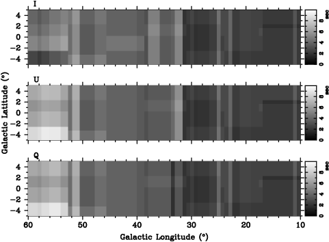
Figure 1: Effective integration time in sec for $I$, $U$ and $Q$ from top to bottom. The time was scaled by a factor of 0.5 in case the observations were made with a reduced bandwidth of $\Delta\nu=295$ MHz.

2.2 Instrumental polarization

Instrumental effects related to the properties of the Urumqi telescope, the $\lambda$6 cm feed and receiving system cause polarization from unpolarized sources. Thus intrinsically unpolarized H II regions show polarized intensity, which exhibits a ring-like pattern for compact sources. The radius of the ring is about that of the beam width and the maximum intensity is measured to be less than 3% of the peak value of total intensity (Sun et al. 2006). Instrumental polarization at this level is not important towards the anti-centre region, where just a few strong sources are located. In the inner Galaxy, however, there are many strong compact H II regions, which together add up so that their instrumental polarization becomes significant and a proper cleaning is required.

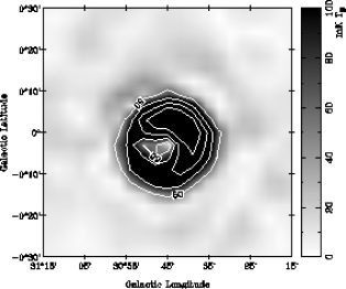
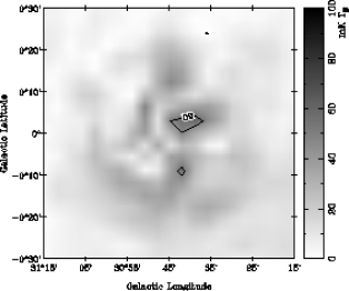
Figure 2: Example of instrumental polarization cleaning applied to the $\lambda$6 cm survey polarized intensity data for the case of the H II region G30.7$-$0.1. The upper panel shows the original polarized intensity and the lower panel the cleaned map. The contours start at 50 mK $T_{\rm B}$ and run in steps of 50 mK $T_{\rm B}$.

The cleaning method we applied has already been described in Paper I in some detail. By observing unpolarized calibrators we obtained maps of total intensity ($I_{\rm cal}$) and polarization ($U_{\rm cal}$ and $Q_{\rm cal}$). Here the polarization is assumed to be completely from instrumental impurity, which can be quantitatively represented as the convolution between the total intensity of the calibrator and the instrumental terms ($U_{\rm inst}$ and $Q_{\rm inst}$) as $U_{\rm cal}=I_{\rm cal}\otimes U_{\rm inst}$ and $Q_{\rm cal}=I_{\rm cal}\otimes Q_{\rm inst}$. We performed a de-convolution in the Fourier domain to derive the instrumental terms. We convolved the survey total intensity maps with the instrumental polarization terms to determine the instrumental polarization, and subtracted these instrumental contributions from the observed polarization maps to obtain the cleaned maps. This method was already successfully applied earlier by Sofue et al. (1987).

We used the H II region RCW 174 ($l=28\aas@@fstack{\circ}8$, $b=3\aas@@fstack{\circ}5$) as calibrator, which shows a high signal-to-noise ratio. It was used to clean the survey maps fairly well. In Fig. 2 we show the elimination of the instrumental polarization for the H II region G30.7$-$0.1. The total intensity of this H II region is about 11 K T_B, and the polarized intensity caused by instrumental effects is about 0.3 K T_B, which is reduced to about 0.06 K T_B, or about 0.5%, after cleaning.

Generally the residual instrumental polarization is well below 1% for the cleaned maps. Sources with total intensities larger than 250 mK $T_{\rm B}$ have a residual polarization at about the 5$\sigma$ level. Compared to the large fluctuations of diffuse polarized intensities along the Galactic plane these residual instrumental effects are usually negligible.

3 Survey results

As described above $I$, $U$ and $Q$ intensities were set to zero at both latitude ends ($b=\pm 5\degr$), because of baseline fitting to remove the ground radiation contributions. This implies that the maps have a relative zero-level. For $I$ maps this is equivalent to an intensity offset, though the observed small-scale structures are not influenced. Thus zero-level setting for total intensity is only crucial when the diffuse emission is quantitatively assessed as we do below to separate thermal and non-thermal emission (see Sect. 6). However, polarized intensities and polarization angles depend on $U$ and $Q$ non-linearly, so that their morphology and structures were significantly changed due to the missing large-scale emission (e.g. Reich 2006). It is thus essential to recover it for a correct physical interpretation.

3.1 Zero-level restoration for $U$ and $Q$

Unfortunately no $\lambda$6 cm polarization data exist at an absolute zero-level, which we might refer to. The on-going C-Band All-Sky Survey (CBASS) is expected to provide the missing large-scale emission. The CBASS has a resolution of $44\arcmin$ and a sensitivity of about 0.1 mK, which is very similar to that of the Urumqi $\lambda$6 cm polarization survey when smoothed to the same angular resolution. Thus the CBASS data are well suited for zero-level restoration. However, as shown later, the required absolute zero-level of polarization at $\lambda$6 cm must be accurate to about 1 mK to be superior to the zero-level restoration scheme we present in the following.

We developed a calibration scheme for the $\lambda$6 cm survey in Paper I, where the correct zero-levels of $U$ and $Q$ were tied to the three-year WMAP K-band (22.8 GHz) data (Page et al. 2007). Now we used the more precise five-year WMAP results (Hinshaw et al. 2009). The K-band polarization data include all large-scale structures. We calculated the corresponding polarized intensities at 4.8 GHz including all large-scale components ($PI\rm^{4.8\,GHz}_{zero}$) by:

$$PI{\rm{}^{4.8\,GHz}_{zero}}=PI{\rm{}^{22.8\,GHz}}\left(\frac{4.8}{22.8}\right)^{\beta_{PI}},$$ (1)

and subsequently for $U$ and $Q$:

$$\begin{array}[]{rcl}U\rm^{4.8\,GHz}_{zero}&=&PI\rm^{4.8\,GHz}_{zero}\sin\left(2\psi^{22.8\,GHz}+\mathcal{R}\lambda^{2}\right)\\[14.22636pt] Q\rm^{4.8\,GHz}_{zero}&=&PI\rm^{4.8\,GHz}_{zero}\cos\left(2\psi^{22.8\,GHz}+\mathcal{R}\lambda^{2}\right).\end{array}$$ (2)

$\psi$ is the polarization angle, and $\beta_{PI}$ is the spectral index for the polarized intensity ($T\propto\nu^{\beta}$ with $T$ being the brightness temperature and $\nu$ the frequency) and $\mathcal{R}$ is the Faraday depth. Assuming the interstellar medium to be a uniform slab, the Faraday depth and RM observed from diffuse polarized emission are related $\mathcal{R}=2\rm RM$ (Sokoloff et al. 1998). For extragalactic sources and pulsars the Faraday depth is equivalent to RM.

As already described in Paper I, we convolved the $U$ and $Q$ maps of both the $\lambda$6 cm survey and the WMAP K-band survey to a resolution of $2\degr$, calculated the intensities according to Eqs. (1) and (2), estimated the differences to the observed $\lambda$6 cm maps, and finally added the differences to the original $U$ and $Q$ $\lambda$6 cm maps. However, towards the inner Galaxy significant depolarization might occur even at $\lambda$6 cm. The observed polarized $\lambda$6 cm emission originates at shorter distances than that observed at K-band. In this case, the above scheme needs to be modified, otherwise too much polarization will be added. We therefore need to determine the spectral index of the polarized intensity, investigate the polarization horizons at both wavelengths, and check the Faraday depths before applying any zero-level restoration.

3.1.1 Spectral index of polarized intensity

Diffuse polarized emission originates from Galactic synchrotron radiation, while total intensities are a mixture of synchrotron and free-free emission. Therefore the total intensity spectral index is not that of the synchrotron emission. Polarization observations at low frequencies suffer from significant depolarization, and are thus not suited to determine the synchrotron spectral index. At high frequencies, polarized intensities are usually very weak because of the generally steep spectrum. Fortunately in the inner Galaxy polarized emission at both the WMAP K- and Ka-band (33 GHz) (Hinshaw et al. 2009) is strong enough for this purpose.

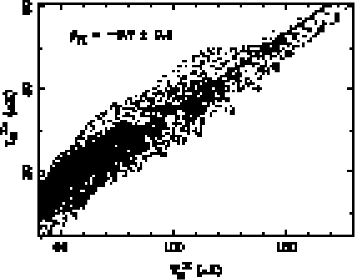
Figure 3: TT-plot between WMAP K-band (22.8 GHz) and Ka-band (33 GHz) for polarized intensities for the region of $40\degr\leq l\leq 60\degr$ (upper panel) and $10\degr\leq l\leq 30\degr$ (lower panel) within the latitude range of $|b|\leq 5\degr$.

We performed TT-plots (Turtle et al. 1962) for polarized intensity between K- and Ka-band for every $10\degr\times 10\degr$ section for the region $10\degr<l<60\degr$ and $|b|<5\degr$, and found a trend of steepening of spectral index from larger to smaller longitudes. The transition region is between longitudes $30\degr$ and $40\degr$. For the same area Reich & Reich (1988a) reported a spectral steeping in total intensity between 408 MHz and 1420 MHz. We modelled the spectral index as follows: For the region $10\degr\leq l\leq 30\degr$, the spectral index is $\beta_{PI}=-3.1$, for the region $40\degr\leq l\leq 60\degr$, the spectral index is $\beta_{PI}=-2.7$ (Fig. 3), and for the transition region the spectral index is a linear interpolation between $-2.7$ and $-3.1$. Note that the spectral index error for the region $10\degr\leq l\leq 30\degr$ is $\Delta\beta=0.1$ from the TT-plot, but increased to $\Delta\beta=0.4$ for the area $40\degr\leq l\leq 60\degr$ caused by a lower signal-to-noise ratio there.

At K- and Ka-bands, depolarization is negligible and the polarization from spinning dust can be neglected as well (Gold et al. 2010). This means that polarized emission at both bands shows intrinsic synchrotron emission. The spectral index derived from polarization data applies also for the Galactic total intensity synchrotron emission component, i.e. $\beta_{\rm syn}=\beta_{PI}$.

3.1.2 Polarization horizon

To check whether the $\lambda$6 cm and K-band surveys observe polarized emission from the same polarization horizon, we performed simulations to show polarized intensities at these two frequencies versus distances for several directions along the Galactic plane. The simulations were based on the hammurabi code developed by Waelkens et al. (2009) and the new Galactic 3D-emission model developed by Sun et al. (2008) using the modifications for high-resolution simulations for selected patches by Sun & Reich (2009), where a Kolmogorov spectrum for the random magnetic fields was included. For each line of sight, the complex polarization $\mathcal{P}$ was calculated following Sun et al. (2008) as,

$${\mathcal{P}=\int_{0}^{r_{\rm max}}P(r)\exp\left(2\mathbf{i}(\psi_{0}(r)+{\rm RM}(r)\lambda^{2})\right){\rm d}r},$$ (3)

where $P(r)$ is the polarized intensity at $r$, $\psi_{0}(r)$ is the intrinsic polarization angle, and the integral was conducted from the observer to a specified distance of $r_{\rm max}$ along the line of sight. The polarized intensity is the absolute value of $\mathcal{P}$. The positions were selected to be in the plane and above the plane at latitudes of about $5\degr$ and longitudes between $10\degr$ and $60\degr$. The simulations have an angular resolution of about $30\arcsec$. The results are shown in Fig. 4, where the data were averaged for an area with a radius of $0\aas@@fstack{\circ}1$ centred at the coordinates marked in each panel. As explained by Sun & Reich (2009) the coordinates of the target patches for simulations had to be adapted to the HEALPix (Górski et al. 2005) projection scheme. The polarized intensities at 22.8 GHz were scaled to 4.8 GHz with a spectral index detailed in Sect. 3.1.1 to facilitate the comparison.

Figure 4: Simulated polarized intensity at $\lambda$6 cm (4.8 GHz) and K-band (22.8 GHz) versus distance for various directions as indicated by the Galactic coordinates in each panel. The dotted lines show the polarized intensity at K-band scaled to $\lambda$6 cm with a spectral index as modelled in Sect. 3.1.1. The solid lines show $PI$ at $\lambda$6 cm.

Figure 4 shows that at $\lambda$6 cm the polarization horizon in the Galactic plane is about 3 kpc for $10\degr\leq l\leq 30\degr$ and increases to about 5 kpc for $40\degr\leq l\leq 60\degr$. Below we adopt 4 kpc as the $\lambda$6 cm polarization horizon for discussion. Figure 4 also shows that about 20%–30% of the intrinsic Galactic polarized emission is observed in the Galactic plane at $\lambda$6 cm. Above the Galactic plane at latitudes of about $5\degr$, only less than about 20% of polarized emission is missed when compared to the scaled K-band data. At the latitude edges of the $\lambda$6 cm survey the polarized emission traced at both wavelengths originate from volumes which are not significantly different.

3.1.3 Faraday depth

The Faraday depth in a certain direction can be estimated from RMs of extragalactic sources, pulsars and diffuse emission. RMs of extragalactic sources contain all contributions along the line-of-sight from the Sun to the Galactic outskirts. However, the polarization horizon inferred from the simulations is about 4 kpc at $\lambda$6 cm, which is shorter than the path length across the Galaxy. Therefore RMs of extragalactic sources cannot be used directly. We retrieved RMs of pulsars in the region of $10\degr<l<60\degr$ and $|b|<5\degr$ from the ATNF pulsar catalogue (Manchester et al. 2005). The distances of these pulsars were estimated by using the NE2001 Galactic electron density model (Cordes & Lazio 2002). Pulsar RMs versus distances are displayed in Fig. 5. The average Faraday depth at distances up to the $\lambda$6 cm polarization horizon of 4 kpc was estimated from the standard deviation of pulsar RMs (excluding one RM outlier of 580 rad m^-2) to be about 22 rad m^-2. This corresponds to an angle rotation of about $5\degr$ at $\lambda$6 cm and we conclude that the Faraday depth in Eq. (2) can be neglected.

Figure 5: Pulsar RMs versus distance based on the NE2001 electron density model. For most of the data the RM error bars are too small to be seen.

Variations of the Faraday depth with longitude cannot be reliably obtained from the small number of pulsar RMs shown in Fig. 5. We simulated $U$ and $Q$ maps at 4.8 GHz and 22.8 GHz using the Galactic 3D-emission models by Sun et al. (2008), derived polarization angle maps at both frequencies, and calculated the RM map. RMs are found to be within $\pm 10$ rad m^-2 from $10\degr$ longitude to $50\degr$ longitude, which is consistent with the result obtained from pulsar RMs. From $l=50\degr$ to $l=57\degr$ the RMs can be as large as about 50 rad m^-2 corresponding to an angle rotation of about $11\degr$, which in principle should be accounted for. As shown below, the zero-level correction to be added to $U$ and $Q$ for this region is less than 1 mK $T_{\rm B}$, which is about twice the rms-noise. Therefore we neglect this RM correction.

3.1.4 A modified scheme for $U$ and $Q$ zero-level restoration

Because of the different polarization horizons at $\lambda$6 cm and at K-band in the Galactic plane, the scaled difference to the K-band polarized emission cannot be used for a correction of the polarization zero-levels. We thus modified the correction scheme of Paper I by referring to the high-latitude regions between $4\aas@@fstack{\circ}5\leq|b|\leq 5\degr$, where the $\lambda$6 cm and K-band surveys observe polarized emission from nearly the same volume. A similar modification was made in Paper II, where the polarized emission in the plane is very weak.

We obtained the differences between the $\lambda$6 cm and K-band $U$ and $Q$ maps for the two high-latitude regions. The correction values were calculated by linear interpolation along latitude and added to the original $U$ and $Q$ data. The $U$ and $Q$ corrections averaged from the difference maps for $4\aas@@fstack{\circ}5\leq|b|\leq 5\degr$ are plotted versus longitude in Fig. 6. The values shown in Fig. 6 are the maximal and minimal corrections for $U$ and $Q$ being applied for each latitude scan. For the region of $50\degr\leq l\leq 60\degr$ the average correction is about 0.6 mK $T_{\rm B}$ for $U$ and 0.8 mK $T_{\rm B}$ for $Q$, which justifies to neglect a Faraday depth dependent correction in view of the rms-noise of 0.5 mK $T_{\rm B}$.

Figure 6: Longitude profiles showing $U$ and $Q$ corrections averaged for $4\aas@@fstack{\circ}5\leq|b|\leq 5\degr$ (see Sect. 3.1.4. for details).

In Fig. 7 we show the pixel distributions of polarized intensities and polarization angles. The distributions with and without adding the large-scale components are quite similar. This result largely differs from that obtained for the survey regions of the outer Galaxy as presented in Papers I and II, where the large-scale corrected polarization angle distribution peaks at $0\degr$.

Figure 7: Pixel distribution of polarized intensities (top) and polarization angles (bottom) before and after baseline restoration.

3.1.5 Accuracy of the zero-level restoration scheme

The spectral index of polarized intensity has an uncertainty of $\Delta\beta=0.1$ for the inner region $10\degr<l<30\degr$. This corresponds to a restoration uncertainty of less than 20% or about 2 mK $T_{\rm B}$ for areas where the $U$ and $Q$ values are as high as 10 mK $T_{\rm B}$ (Fig. 6). For the outer region $40\degr<l<60\degr$, the spectral index has a large uncertainty of $\Delta\beta=0.4$, but the typical added $U$ and $Q$ values are around 1 mK $T_{\rm B}$ (Fig. 6). This again means an uncertainty of about 2 mK $T_{\rm B}$ for the zero-level. To summarize: the uncertainty of the applied zero-level restoration for the entire survey region caused by the spectral index uncertainty used in the extrapolation from WMAP frequency towards 4.8 GHz is up to the $4\times\sigma$ level of the observed polarized intensity, but mostly below.

Based on the simulations presented in Sect. 3.1.2, the $\lambda$6 cm survey could miss up to about 20% of polarized intensity at the latitude edges. This is equivalent to a spectral index uncertainty of about $\Delta\beta=0.1$. As already shown above, this does not have a significant influence on the results.

When the CBASS $\lambda$6 cm polarization survey becomes available, missing large-scale components of this survey can be added without extrapolation over a wide frequency range. Compared to the present extrapolation method, an improvement will be obtained in case the zero-level in $U$ and $Q$ can be measured with an accuracy better than 2 mK.

3.2 Overview of the survey maps

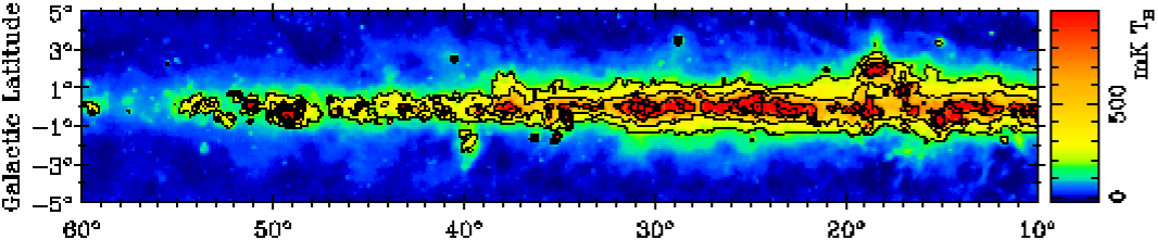
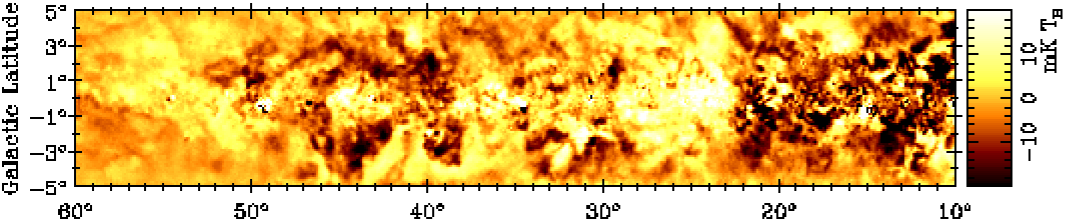
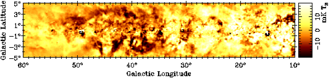
Figure 8: Maps at $\lambda$6 cm for the region $10\degr\leq l\leq 60\degr$. From top to bottom $I$, $U$ and $Q$ maps are shown as observed. Overlaid contours on the $I$ map run in steps of $2^{n}\times 200$ mK $T_{\rm B}$ with $n=0,\,1,\,2,\,\ldots$.

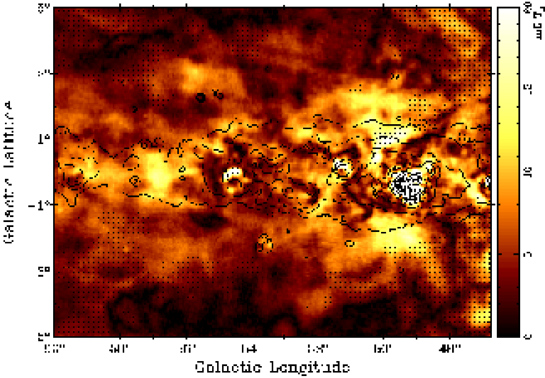
Figure 9: Zero-level restored $PI$ maps overlaid by total intensity contours and bars showing B-vectors. The contours run in steps of $2^{n}\times 50$ mK $T_{\rm B}$ with $n=0,\,1,\,2,\,\ldots$. The lengths of B-vectors are proportional to $PI$. Below an intensity cutoff of 2.5 mK $T_{\rm B}$ (5$\times$rms-noise) no bars are shown.

Figure 10: The same as Fig. 9 for the lower longitude regions.

$I$, $U$ and $Q$ maps are shown in Fig. 8. $PI$ maps calculated from the zero-level restored $U$ and $Q$ maps are shown in Figs. 9 and 10. The $I$ maps show strong diffuse emission concentrated along the ridge of the Galactic plane, where a high density of discrete sources such as H II regions and supernova remnants (SNRs) is seen. The emission increases towards lower longitudes. The longitude profile for $I$ averaged within $b=\pm 2\degr$ is compared with that of the Parkes $\lambda$6 cm survey (Haynes et al. 1978) in Fig. 11. The total intensity structures agree quite well. The TT-plot yields an intensity ratio of $1.0\pm 0.1$ and an arbitrary offset of about 1000 mK (which was added to the Parkes data release). This proves in addition that both $\lambda$6 cm surveys are consistent.

Figure 11: Total intensity $I$ along Galactic longitude averaged within $b=\pm 2\degr$. The solid line shows the $\lambda$6 cm survey data and the dotted line the Parkes survey (Haynes et al. 1978) data with an offset of about 1000 mK.

Polarized emission shows different structures compared to those seen in total intensity (Figs. 9 and 10). There is strong polarized emission even far above the plane, which is similar to that seen in the Effelsberg $\lambda$11 cm survey maps (Junkes et al. 1987; Duncan et al. 1999). However, the polarized structures revealed by these two surveys do not correspond to each other, because of different base-line settings and polarization horizons. A $10\degr$-region centred at $l=50\degr$, $b=0\degr$ has been observed as part of the Toruń $\lambda$6 cm survey project (Ryś et al. 2006). The most prominent polarized structures, such as the patch at $l=49\aas@@fstack{\circ}80$, $b=1\aas@@fstack{\circ}15$, agree with our $\lambda$6 cm polarization survey.

It is evident that the B-vectors do not align well with the Galactic plane, which is either intrinsic or caused by strong Faraday rotation along the line-of-sight.

The most prominent structures are,

1. Structures visible in both total and polarized intensities: These are point sources and SNRs. Particular bright are G34.7$-$0.4 (W 44), G39.7$-$2.0 (W 50) and G54.4$-$0.3 (HC 40). A weak polarized filament is traced from $l=23\aas@@fstack{\circ}5$, $b=5\degr$ towards lower latitudes. This filament was previously identified as an extension of the North Polar Spur (NPS) by total intensity observations at $\lambda$21 cm by Sofue & Reich (1979). For the first time we are able to trace this filament also in polarization.

2. Polarized patches without corresponding total intensities: The patches span wide scales from tens of arcmin to several degrees. Most of them are seen outside of the Galactic plane ridge. More patches are seen at low longitudes than at large longitudes. These patches are probably produced by turbulent fields as discussed below.

3. Narrow depolarization regions commonly called “canals”: They are most pronounced in the region around $11\degr<l<15\degr$. These canals are not related to total intensity structures. As demonstrated later an abrupt polarization angle change by about $0.6\pi$ over $3\arcmin$ can cause such canals.

4. Large depolarized regions we call “voids”: Most voids do not correspond to a total intensity minimum or other feature. An example is seen at $l=40\aas@@fstack{\circ}9$, $b=-4\aas@@fstack{\circ}2$. These regions were modeled in Sect. 5.2 by the Faraday Screen model already used in Papers I and II.

4 Discrete objects

For point-like or compact sources, flux densities were obtained by fitting a two-dimensional elliptical Gaussian. A list of compact sources from the entire survey will be presented in a forthcoming paper. Studies of SNRs located in this area will also be presented in subsequent papers. Other discrete objects such as the NPS extension as well as H II regions will be discussed in this section. Polarized structures with no counterparts in total intensity are analysed in Sect. 5.

4.1 Extended sources in general

Prominent extended sources are either SNRs or H II regions. Their spectra differ and can be used to identify them. Shell-type SNRs are non-thermal sources with spectral indices close to $\alpha\sim-0.5$, whereas H II regions are thermal with nearly flat spectra. The spectra of strong sources can be determined by their integrated flux density at several frequencies. For weak sources, whose flux density cannot be determined very well, we investigated their spectra by TT-plots and fit their slopes. The maps throughout the paper were smoothed to $9\aas@@fstack{\prime}5$ required to perform TT-plots. The TT-plot method largely circumvents the influence of background emission differences amongst maps from different surveys. Plerions and pulsar wind nebulae (PWNe) are non-thermal SNRs, but exhibit flat spectra similar to H II regions. However, all types of SNRs are polarized and show X-ray emission, while H II regions are usually associated with strong infrared sources. The ratio of IRAS 60 $\mu$m to radio continuum intensity is usually much larger for H II regions than for SNRs (e.g. Fürst et al. 1987). We used X-ray images from the ROSAT all-sky survey and high-resolution IRAS 60 $\mu$m maps (Cao et al. 1997) to distinguish between SNRs and H II regions.

4.2 H II regions

H II regions reside predominantly in spiral arms and thus numerous H II regions are seen in the present survey section as the line-of-sight intersects many spiral arms (Hou et al. 2009). Most of the known H II regions have been catalogued by Paladini et al. (2003) and Hou et al. (2009). They are visible in the $I$ maps. Some emission complexes, as for example the W 51 complex centred at $l=49\aas@@fstack{\circ}2$, $b=-0\aas@@fstack{\circ}4$, host many individual H II regions surrounded by diffuse emission. Such a study is beyond the scope of this paper. The $\lambda$6 cm survey reveals some previously unknown large and weak H II regions as demonstrated by Shi et al. (2008). However, some efforts are required to discover new H II regions in the current region because of obscuration by strong diffuse emission. Therefore we limit our investigation to two objects out of the Galactic plane or longitudes close to $l=60\degr$, where the diffuse emission is weaker.

We identified two thermal structures in this survey region, which could be new H II regions. The first one, G12.8$-$3.6, at $l=12\aas@@fstack{\circ}75$, $b=-3\aas@@fstack{\circ}55$, has a size of about $100\arcmin\times 24\arcmin$ (Fig. 12). Its integrated flux density is difficult to measure because of its complex environment. The spectral index from a TT-plot between the $\lambda$6 cm and Effelsberg $\lambda$11 cm data is $\alpha=0.15\pm 0.29$, which indicates that the source is thermal. The object is at the latitude limit of the Effelsberg $\lambda$21 cm survey, which was not used for the analysis. The thermal nature of G12.8$-$3.6 is further corroborated by infrared emission at 60 $\mu$m coinciding exactly with the radio emission (Fig. 12). The second source, G56.7$-$0.6, located at $l=56\aas@@fstack{\circ}70$, $b=-0\aas@@fstack{\circ}60$, has an apparent size of about $65\arcmin\times 27\arcmin$ (Fig. 13). The flux densities measured from the $\lambda$6 cm survey and Effelsberg $\lambda$11 cm and $\lambda$21 cm surveys are 1.76$\pm$0.09 Jy, 1.32$\pm$0.07 Jy, and 1.96$\pm$0.11 Jy, respectively, which yields a spectral index of $\alpha=0.08\pm 0.06$. Unfortunately we cannot find exciting stars for both structures from other database.

Figure 12: IRAS 60 $\mu$m greyscale image showing the H II region G12.8$-$3.6. Contours display total intensities at $\lambda$6 cm starting at 10 mK $T_{\rm B}$ and running in steps of 10 mK $T_{\rm B}$.

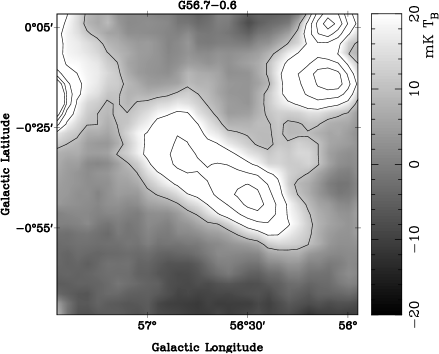
Figure 13: $\lambda$6 cm total intensity image for the newly identified H II region G56.7$-$0.6 shown in greyscale and contours, which start at 10 mK $T_{\rm B}$ running further in steps of 10 mK $T_{\rm B}$.

Another object G57.7+0.3 was already proposed by Sieber & Seiradakis (1984) to be a H II region, but was not catalogued by Paladini et al. (2003). We measured flux densities at $\lambda$6 cm and Effelsberg $\lambda$11 cm and $\lambda$21 cm surveys to be 2.51$\pm$0.13 Jy, 2.33$\pm$0.13 Jy, and 2.54$\pm$0.20 Jy, respectively. The spectral index is $\alpha=0.00\pm 0.07$. Strong infrared emission is associated, we therefore confirm this source to be a H II region.

4.3 The southern North Polar Spur extension

The North Polar Spur (NPS) is most probably a local and very old SNR (Salter 1983). Its filamentary shell structure should not be affected when running across the Galactic plane. However, the strong emission from unrelated more distant Galactic plane emission causes confusion that it becomes very difficult to trace the NPS in this area. This was already demonstrated by $\lambda$21 cm observations by Sofue & Reich (1979). At $\lambda$6 cm confusion is less strong, so that the filamentary southern NPS extension can be traced from $l=23\degr$, $b=5\degr$ towards a latitude of about $2\aas@@fstack{\circ}5$ in total intensity. At lower latitudes it is confused with strong diffuse emission (Fig. 14). The NPS extension can be traced also by its polarization towards a lower latitude of about $0\aas@@fstack{\circ}5$ and eventually to a latitude of about $-3\degr$. The average polarized intensity is about 15 mK $T_{\rm B}$. At about $l=22\aas@@fstack{\circ}4$, $b=3\aas@@fstack{\circ}6$ the NPS splits into two filaments as seen at $\lambda$21 cm in total intensity (Sofue & Reich 1979). This is also seen at $\lambda$6 cm, where polarization from the two filaments is seen as well. The southern filament is longer and the northern part shorter at $\lambda$6 cm in total intensity than at $\lambda$21 cm. The southern filament is inclined by about $50\degr$ relative to the Galactic plane, while the northern filament is inclined by $30\degr$. The B-vectors are roughly orientated tangential to the northern filament. For the southern filament the B-vector direction is almost parallel to the Galactic plane for latitudes below about $2\aas@@fstack{\circ}5$.

Wolleben (2007) has modeled the NPS by two local shells mainly based on DRAO 1.4 GHz all-sky polarization survey data (Wolleben et al. 2006). However, this polarization survey suffers strong depolarization for latitudes below about $30\degr$, which prevents tracking the NPS towards low latitudes. This global model does not consider splitting of the filamentary shell as observed. Follow-up observations extending the $\lambda$6 cm survey for the higher latitude NPS regions are on the way, that we postpone any further discussion.

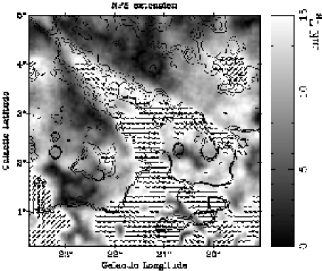
Figure 14: Polarization image for the southern NPS extension. Contours show total intensities and bars represent B-vectors. Contours start at 5 mK $T_{\rm B}$ and run in steps of 4.5 mK $T_{\rm B}$.

5 Polarized structures

5.1 General considerations

The maximum theoretical polarization percentage of synchrotron emission is about 75%. However, random magnetic fields may reduce the polarization percentage significantly. For a ratio of random to regular magnetic fields of 1.5, the intrinsic percentage polarization reduces to about 30% (Sun et al. 2008). We will use this value throughout this paper. Two mechanisms may further smear out polarized emission: depth polarization and beam depolarization.

Depth depolarization occurs when polarized synchrotron emission is mixed with thermal gas. Polarized emission originating at different distances along the line-of-sight experiences a different amount of Faraday rotation and thus different polarization angles. Adding polarized emission components along the line-of-sight causes a reduction up to an entire cancellation of polarization. Quantitatively the amount of depolarization $p$, i.e. the ratio of the observed to intrinsic polarized percentage, can be written as (Sokoloff et al. 1998),

$$p=\frac{1-\exp(-S)}{S},$$ (4)

where $S=2\sigma_{\rm RM}^{2}\lambda^{4}-2{\mathbf{i}}\mathcal{R}\lambda^{2}$, and $\sigma_{\rm RM}$ is the RM scattering along the line-of-sight. If $\sigma_{\rm RM}=0$, Eq. (4) simplifies to $p=\sin(\mathcal{R}\lambda^{2})/\mathcal{R}\lambda^{2}$, which is frequently used.

Beam depolarization occurs by Faraday rotation in front of the synchrotron-emitting medium. RM variations on scales smaller than the beam width result in polarization angle difference. By integration across the beam the observed polarization is reduced. Following Sokoloff et al. (1998) the depolarization factor $p$ can be expressed as,

$$p=\exp(-2\sigma_{\rm RM,\,\bot}^{2}\lambda^{4}),$$ (5)

where $\sigma_{\rm RM,\,\bot}$ is the RM variance across the beam. A rough estimate for $\sigma_{\rm RM,\,\bot}$ can be given as (Gaensler et al. 2001),

$$\sigma_{\rm RM,\,\bot}=\frac{Kn_{e}bL}{2\sqrt{3}}\left(\frac{l}{L}\right)^{1/2},$$ (6)

where $K$ is a constant, $n_{e}$ is the electron density, $b$ is the strength of the random magnetic field, $L$ is the depth through the Faraday rotating medium, and $l$ is the coherent length of the random magnetic fields. The quantity $Kn_{e}bL$ is roughly equal to $\sigma_{\rm RM}$ and $l$ is about the spatial scale resolved by the beam for a distance $L$.

For this $\lambda$6 cm survey section the polarization horizon in the Galactic plane was estimated to be about 4 kpc based on simulations as described by Sun & Reich (2009) (see Fig. 4). At distances larger than 4 kpc the average pulsar RM is about 200 rad m^-2 and the RM variance along the line-of-sight is about 400 rad m^-2 (Fig. 5). With these values a depolarization factor $p$ of about 0.2 is calculated using Eq. (4), which means a quite significant depolarization. The extended H II region W 35 at $l=18\aas@@fstack{\circ}45$, $b=2\aas@@fstack{\circ}05$ is located at a distance of about 2.9 kpc (Müller et al. 1987) and does almost not modulate polarization, which is consistent with the simulated polarization horizon. Synchrotron emission originates at most in spiral arms, so that we see polarized emission from the Sagittarius and the Scutum arms for the inner region and only from the Sagittarius arm for the outer region (see Fig. 15). For the longitude range of $50\degr<l<60\degr$ the line-of-sight is almost tangential to the Sagittarius arm (Fig. 15). It is commonly assumed that the large-scale magnetic fields follow the spiral arms (Han et al. 2006) and thus RM increases. This results in a higher degree of depolarization in this direction.

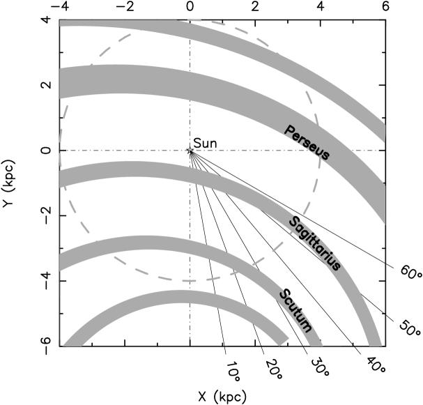
Figure 15: Sketch of the location of Galactic spiral arms taken from the polynomial spiral arm model of Hou et al. (2009). The longitude range of the present survey section is indicated. The dashed circle has a radius of 4 kpc, and indicates the polarization horizon at $\lambda$6 cm in the Galactic plane.

The $\lambda$6 cm maps of this survey section show numerous depolarization features such as voids and canals (Figs. 9 and 10). Within the polarization horizon, depth depolarization is not important, because absolute pulsar RMs and their fluctuations are small. If beam depolarization is significant, we calculate that for a depolarization factor of $p=0.1$ a RM variance across the beam of about 275 rad m^-2 is required (see Eq. (5)). According to Eq. (6) $\sigma_{\rm RM,\,\bot}\approx\sigma_{\rm RM}\sqrt{l/L}/2\sqrt{3}$. Pulsar RMs give $\sigma_{\rm RM}\leq 400$ rad m^-2, and $l/L$ is about the beam size. This implies $\sigma_{\rm RM,\,\bot}\approx 6$ rad m^-2, or $p=1$. We conclude that beam depolarization can be largely neglected.

Most of the Faraday Screens discussed in Paper I and II cause no large depolarization of background emission, but rotate the polarization background position angle. After rotation the polarized background and foreground emission have different polarization angles compared to their surroundings. The observed sum of both components then shows a decrease in polarized intensity. A simple model was described and extensively used in Papers I and II. The positions were defined as “on” if the line-of-sight passes the Faraday Screen and “off” otherwise. In general, the polarized intensity and angle towards “on” and “off” positions can be expressed as,

$$\left\{\begin{array}[]{rcl}PI_{\rm on}&=&\sqrt{PI^{2}_{\rm bg}+PI^{2}_{\rm fg}+2PI_{\rm bg}PI_{\rm fg}\cos(2\psi_{\rm bg}+2\psi_{\rm s}-2\psi_{\rm fg})}\\[11.38109pt] \psi_{\rm on}&=&\displaystyle{\frac{1}{2}{\rm atan}\frac{PI_{\rm bg}\sin(2\psi_{\rm bg}+2\psi_{\rm s})+PI_{\rm fg}\sin 2\psi_{\rm fg}}{PI_{\rm bg}\cos(2\psi_{\rm bg}+2\psi_{\rm s})+PI_{\rm fg}\cos 2\psi_{\rm fg}}}\\[14.22636pt] PI_{\rm off}&=&\sqrt{PI^{2}_{\rm bg}+PI^{2}_{\rm fg}+2PI_{\rm bg}PI_{\rm fg}\cos(2\psi_{\rm bg}-2\psi_{\rm fg})}\\[11.38109pt] \psi_{\rm off}&=&\displaystyle{\frac{1}{2}{\rm atan}\frac{PI_{\rm bg}\sin 2\psi_{\rm bg}+PI_{\rm fg}\sin 2\psi_{\rm fg}}{PI_{\rm bg}\cos 2\psi_{\rm bg}+PI_{\rm fg}\cos 2\psi_{\rm fg}}}\end{array}\right.$$ (7)

A Faraday Screen causes an angle rotation $\psi_{\rm s}={\rm RM_{s}}\lambda^{2}$. The subscripts “fg” and “bg” denote the foreground and background components, respectively. If only data at one frequency are available, the model may be simplified that $\psi_{\rm bg}=\psi_{\rm fg}=\psi_{\rm off}$. For the anti-centre regions as discussed in Paper I and II, the dominating emission originates from the disk field, where the magnetic field is in general parallel to the Galactic plane. This means $\psi_{\rm off}$ is close to $0\degr$.

5.2 Polarized patches

Regions showing strong polarized emission are predominantly “patches”, such as the extended feature centred at $l=43\aas@@fstack{\circ}80$, $b=-2\aas@@fstack{\circ}90$. Most of these patches do not have corresponding total intensity emission. The patches show either intrinsic polarization from a region in interstellar space or they are caused by Faraday Screen modulation of polarized background emission.

We consider a Faraday Screen origin for the patches in general as unlikely. In this scenario polarization angles of the foreground and background components must differ. Faraday Screens have to rotate the polarized background, so that a reduction of the angle difference to the foreground component is obtained. In this case the polarized emission appears to be stronger compared to its surroundings. The survey maps show that the polarized intensity of the patches is in most cases much larger compared to their surroundings. In general the ratio of $PI_{\rm off}/PI_{\rm on}$ is estimated to be less than about 0.3. If foreground and background polarized intensities are nearly identical, their angles should satisfy $\psi_{\rm s}\approx\psi_{\rm fg}-\psi_{\rm bg}\approx 90\degr$ (see Eq. (7)) towards all the patches. It is unlikely that this is true over a wide area. If foreground and background intensities differ significantly a ratio of $PI_{\rm off}/PI_{\rm on}$ less than 0.3 can not be caused by Faraday Screen action at all. The RMs of the Faraday Screens have to be less than 200 rad m^-2 as inferred from pulsar RMs (Fig. 5). This results in a maximum angle rotation by a Faraday Screen of about $45\degr$ at $\lambda$6 cm. Moreover it is generally believed that the magnetic field perpendicular to the plane is much smaller than that parallel to the plane (e.g. Han & Qiao 1994; Han et al. 1999; Sun et al. 2008). Thus angle differences between background and foreground shall approach zero. Therefore the patches are unlikely to be produced by Faraday Screens.

Thus we consider the patches in their majority as intrinsically polarized features. Since they have no correspondence in total intensity, they are not caused by polarized objects such as SNRs. Instead we consider the patches as diffuse synchrotron emission components originating from turbulent field cells, whose power spectrum follows a power-law with a non-zero spectral index. The synchrotron emission observed from various turbulent field cells with different magnetic field orientations is smooth or almost structureless in total intensity. Polarized emission, however, shows irregularities or inhomogeneities depending on the field orientation in the different cells and their correlation. As shown by high angular resolution simulations by Sun & Reich (2009), turbulent magnetic fields with a Kolmogorov-like spectrum produce polarized features without corresponding total intensity. In the anti-centre region the cosmic ray electron density is low and the polarized intensities contributed by individual turbulent field cells is small as well. Therefore we do not expect to see many polarized patches, which is consistent with the $\lambda$6 cm observations presented in Papers I and II. At K-band the polarization horizon is large everywhere in the Galaxy. Many turbulent cells along the line-of-sight average out all distinct structures and thus individual polarized patches are not expected to be seen in the WMAP maps (Hinshaw et al. 2009), what is in agreement with the observations.

Figure 16: $U$, $Q$ and $PI$ structure functions for the present $\lambda$6 cm survey section. The structure functions calculated for smoothed ($9\aas@@fstack{\prime}5$) and original ($4\aas@@fstack{\prime}3$) angular resolution $\lambda$11 cm $PI$ data are also shown.

We apply structure functions to study the properties of the polarized patches following the approach by Sun & Reich (2009). It is yet unknown how the turbulent magnetic field properties are reflected in structure functions. The structure functions are not influenced by missing large-scale components, so that the analysis was based on the original maps. The structure functions for $U$, $Q$ and $PI$ at $\lambda$6 cm are shown in Fig. 16. For comparison we retrieved the Effelsberg $\lambda$11 cm $U$ and $Q$ data for this survey region, smoothed them to the same angular resolution as the $\lambda$6 cm survey and re-calculated polarized intensity. The structure function for the smoothed $PI$ at $\lambda$11 cm as well as the original with an angular resolution of $4\aas@@fstack{\prime}3$ are also shown in Fig. 16. All structure functions can be described by a power-law. The spectral index is about 0.3 for the $9\aas@@fstack{\prime}5$ angular resolution data and 0.1 for the $4\aas@@fstack{\prime}3$ resolution $\lambda$11 cm $PI$ data. The spectral index refers to spatial scales between about $20\arcmin$ and $3\degr$, which corresponds to sizes of about 20 pc and 200 pc for the polarized patches in case their distance is 4 kpc.

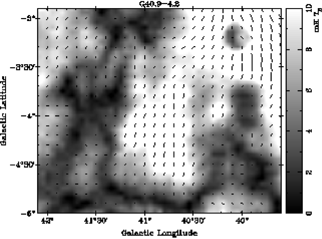
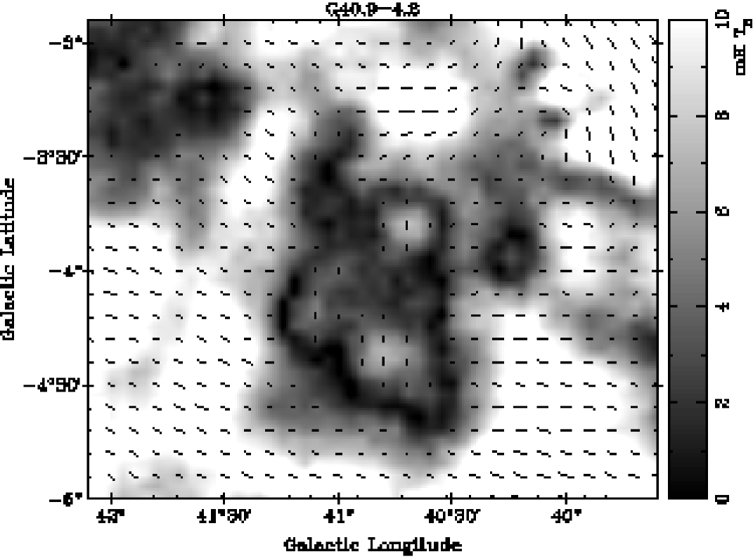
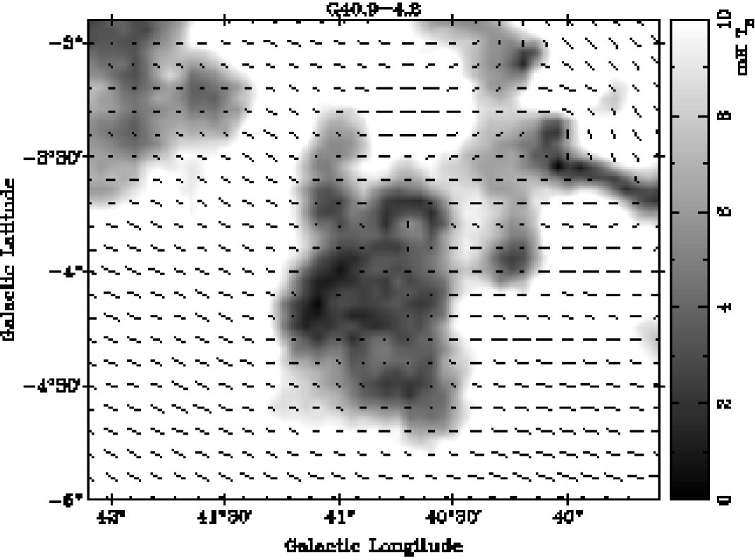
Figure 17: Polarized intensity maps for the void G40.9$-$4.2. The upper panel shows the original map, the middle panel shows the map with the zero-level restored with a spectral index of $\beta_{PI}=-2.7$ according to the restoration model discussed in Sect. 3.1.1. The lower panel shows the map with the zero-level restored using the lowest possible spectral index of $\beta_{PI}=-3.1$ (see Fig. 3). $PI$ is always shown in grey scale, and bars indicate polarization B-vectors.

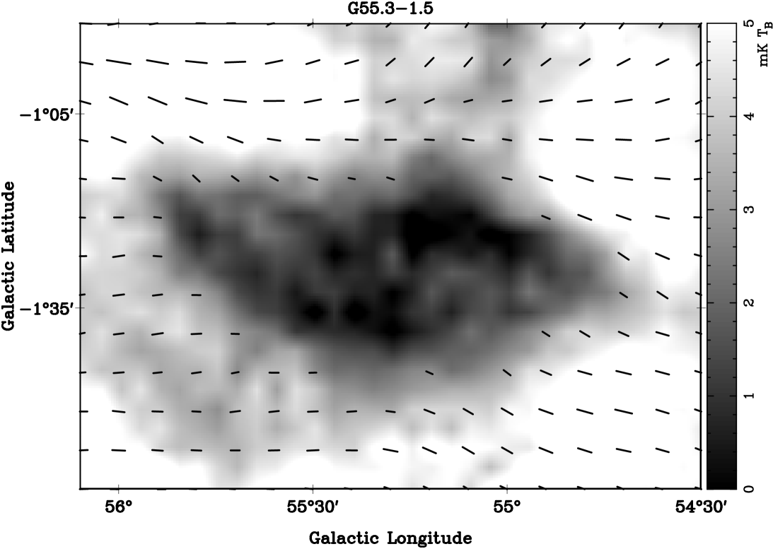
Figure 18: Polarization void G55.3$-$1.5. $PI$ is shown in grey scale, and bars indicate polarization B-vectors.

The morphology of patches resulting from turbulent magnetic field cells should vary with frequency and resolution. The statistical properties such as the slope of the structure function should be independent on frequency. However, statistics depend on angular resolution. For low angular resolutions polarized patches from nearby turbulent field cells dominate, which will cause a steepening of the spectrum of the structure function. The slope of the $\lambda$11 cm structure functions in logarithmic scale changed from about 0.1 to 0.24 after smoothing, consistent with the above expectation. The slope of 0.24 for smoothed $\lambda$11 cm $PI$ is almost the same, compared to 0.3 as calculated for the $\lambda$6 cm polarization data. This result supports our argument that polarized patches reflect turbulent field cells. The slight discrepancy between $\lambda$11 cm and $\lambda$6 cm may stem from differences of their polarization horizon and the corresponding different emission volumes. Simulations were made as described in Sect. 3.1.2, which indicate that the polarization horizon at $\lambda$11 cm is about 1–3 kpc compared to about 4 kpc at $\lambda$6 cm.

5.3 Large polarization voids

We define “voids” as large almost completely depolarized regions without correspondence in total intensity. Previously Stil & Taylor (2007) reported on regions of about $10\degr$ in size, where the density of extragalactic sources from the NVSS is reduced by a factor 2–4. The size of these polarization shadows indicates a local origin for the depolarization and Stil & Taylor (2007) discussed several possibilities. The voids seen at $\lambda$6 cm could neither be caused by depth nor by beam depolarization as discussed above. Instead we use the Faraday Screen model described above to understand the polarization voids.

The void G40.9$-$4.2, located at $l=40\aas@@fstack{\circ}85$, $b=-4\aas@@fstack{\circ}15$, has a size of about $55\arcmin\times 40\arcmin$ (Fig. 17). It is almost entirely depolarized towards its centre. To demonstrate the importance of absolute calibration when discussing “voids” we show the original polarized intensity map and the map with large-scale emission added in Fig. 17. The void G40.9$-$4.2 appears as a polarized emission feature in the original map and turns into a depression when large-scale components were added. Instead of using the spectral index of $\beta_{PI}=-2.7$ we also show the large-scale level restored with a spectral index of $\beta_{PI}=-3.1$ (lower panel in Fig. 17), which is the lower spectral index limit for this longitude range (see Sect.  3.1.1). As shown in Fig. 17 the “void” slightly shrinks in size, but its morphology remains almost unchanged. This demonstrates that the uncertainties related to the spectral index determination do not have a large influence on the analysis of polarized structures.

Another outstanding example of a void is G55.3$-$1.5 located at $l=55\aas@@fstack{\circ}30$, $b=-1\aas@@fstack{\circ}50$ (Fig. 18). Its size is about $51\arcmin\times 22\arcmin$. The polarized emission drops close to zero towards its centre direction. In this case the large-scale corrections of $U$ and $Q$ are very close to zero and therefore the maps with and without restoration are almost identical.

According to the Faraday Screen model (Eq. (7)) the foreground and background polarized intensity should be almost equal and the polarization angle rotation by the Faraday Screen is $\psi_{\rm s}=90\degr+\psi_{\rm fg}-\psi_{\rm bg}$. The “off” polarization angle should be $\psi_{\rm off}=(\psi_{\rm fg}+\psi_{\rm bg})/2$. For both voids we measured $\psi_{\rm off}\approx 160\degr$, indicating $\psi_{\rm fg}+\psi_{\rm bg}=320\degr$. As both $\psi_{\rm fg}$ and $\psi_{\rm bg}$ are in the range between $0\degr$ and $180\degr$, we obtain $-40\degr\leq\psi_{\rm fg}-\psi_{\rm bg}\leq 40\degr$, and subsequently $50\degr\leq\psi_{\rm s}\leq 130\degr$. The RM of the Faraday Screens needs to be about $220$ rad m^-2 to account for $\psi_{\rm s}=50\degr$, which is about the RM maximum constrained by pulsar RM in this area (Fig. 5). Larger values could not be entirely ruled out, because there are no pulsar RMs measured in the direction of the voids. In case of $\psi_{\rm s}=50\degr$ the angle difference between the foreground and background emission is about $40\degr$. For a smaller angle difference the RM of the Faraday Screens must be larger.

In case the polarized emissivity is uniform along the line-of-sight, the distance to the Faraday Screens is about half of the polarization horizon, or about 2 kpc (Fig. 4). This yields a mean size of about 28 pc for G40.9$-$4.2, and about 21 pc for G55.3$-$1.5. The $\lambda$6 cm brightness temperature contributed by the warm thermal gas from the Faraday Screen can be written as $T=T_{e}\tau=0.13n_{e}^{2}L$ mK. Here the opacity $\tau$ was calculated according to the formula by Rohlfs & Wilson (2004), where $n_{e}$ is the electron density in cm^-3 and $L$ is the size of the Faraday Screen in pc. The electron temperature $T_{e}$ was taken to be 8000 K. The non-detection of the Faraday Screen in total intensity provides an upper limit for the electron density of about 1.2 cm^-3 for G40.9$-$4.2, and 1.4 cm^-3 for G55.3$-$1.5, when taking 5$\times$rms-noise as an upper limit and assuming the depth of the Faraday Screen is the mean of the projected major and minor axes. The resulting lower limits for the regular magnetic field strength along the line-of-sight is then about 8 $\mu$G for G40.9$-$4.2, and 9 $\mu$G for G55.3$-$1.5.

In the above discussions we have assumed uniform emissivity along the line-of-sight. For a local emissivity enhancement (see Sun et al. 2008 for details) the distance to the Faraday Screens is shorter, its size becomes smaller and its regular magnetic field increases.

5.4 Canals

We see copious filamentary polarization minima in the $\lambda$6 cm survey maps, which were named “canals” in previous low-frequency observations (e.g. Haverkorn et al. 2004). The polarized intensity along the canals drops to typically 10%–30% compared to their surroundings. One of the most pronounced canals (see Fig. 9) runs from $l=43\aas@@fstack{\circ}6$, $b=-4\aas@@fstack{\circ}8$ to $l=41\aas@@fstack{\circ}0$, $b=-1\aas@@fstack{\circ}0$. Another striking one is located at $l=33\degr$, $b=-3\aas@@fstack{\circ}5$ (Fig. 9). Many more canals appear towards the lower longitude regions, in particular the region between longitude of $10\degr$ and $13\degr$ (Fig. 10). The length of the canals varies from tens of arcmin to several degrees. The width of the canals is about $5\arcmin$ to about $15\arcmin$, similar to the beam size.

The depolarization along the canals may be attributed to variations of polarization angles across the beam size $D$. Let the angles vary linearly by $\Delta\psi$ over a finite region $x_{0}$, i.e., $\psi(x)=\psi_{0}+\Delta\psi\frac{x}{x_{0}}$, where $|x|\leq x_{0}/2$. The depolarization factor $p$ can then be calculated following Sokoloff et al. (1998) as,

$$p=\frac{\int\limits_{0}^{x_{0}/2D}\exp(ax^{2})\cos(2\Delta\psi_{D}x){\rm d}x+\cos\Delta\psi\int\limits_{x_{0}/2D}^{\infty}\exp(ax^{2}){\rm d}x}{\int\limits_{0}^{\infty}\exp(ax^{2}){\rm d}x},$$ (8)

where $\Delta\psi_{D}=\Delta\psi D/x_{0}$ is the angle increment over the beam $D$, and $a=-4\ln 2$. The results are shown in Fig. 19. The polarization angles around the canals in our maps show sharp variations, where $x_{0}\approx 3\arcmin$ meaning $x_{0}/D\approx 0.3$, and $0.5\pi\lesssim\Delta\psi\lesssim 0.7\pi$. These parameters correspond depolarization factors of 0–0.3 in Fig. 19, which are consistent with the observations.

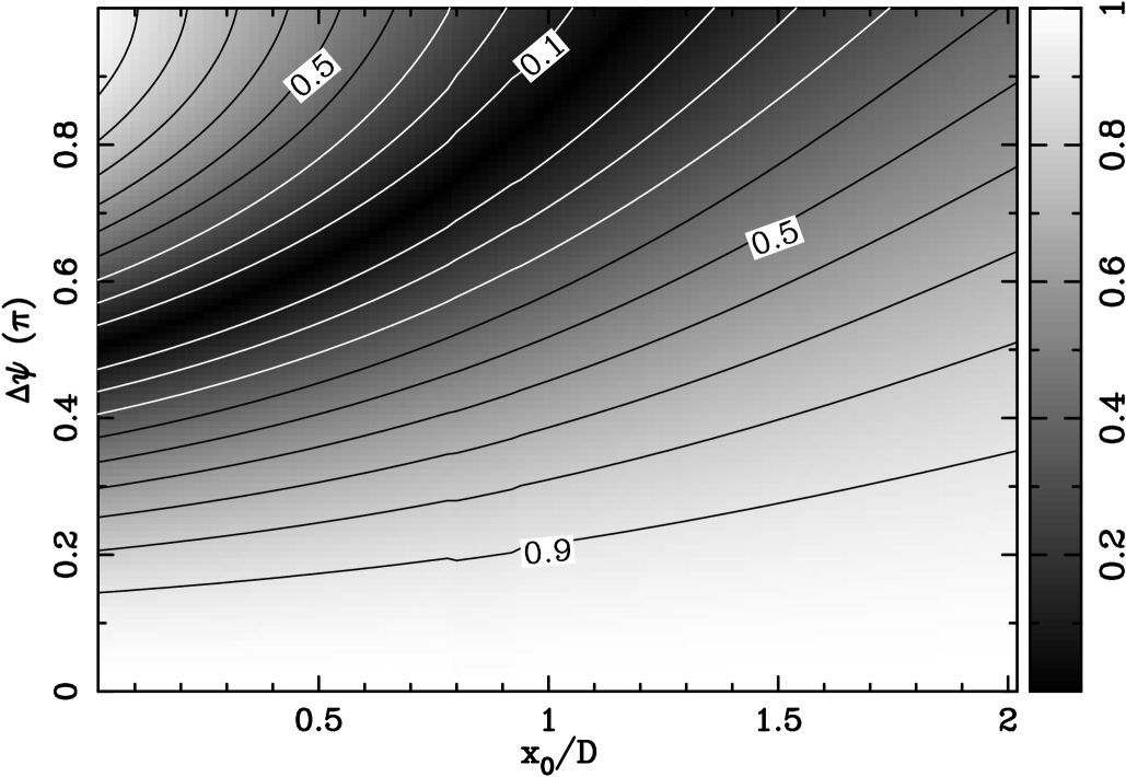
Figure 19: Depolarization factors versus polarization angle change ($\Delta\psi$) across the scale $x_{0}$ and the ratio of $x_{0}$ to the beam size $D$.

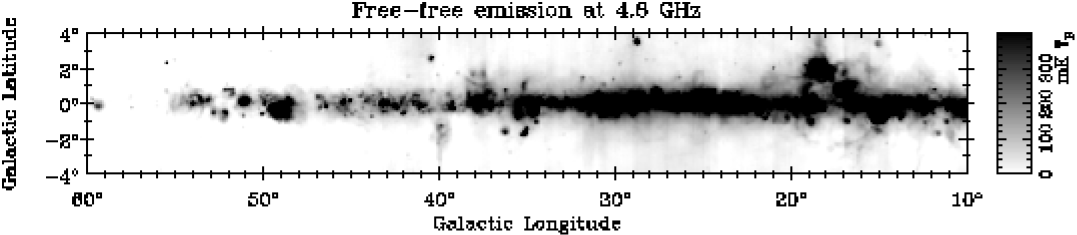
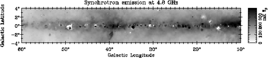
Figure 20: Decomposed thermal (upper panel) and non-thermal component (lower panel) for the $\lambda$6 cm survey between $10\degr\leq l\leq 60\degr$ based on the non-thermal spectral index model in Sect. 3.1.1 and $\beta_{\rm ff}=-2.1$ for optically thin thermal emission.

Variations of polarization angles can be either intrinsic or extrinsic (Haverkorn et al. 2004). At $\lambda$6 cm an angle change of $90\degr$ requires a Faraday depth of about 400 rad m^-2, which is not supported by pulsar RMs for this area. Therefore an intrinsic scenario for the origin of the canals is likely, which means that they are caused by rapid variations of the polarization angle across the beam size. Thus canals delineate boundaries of polarized patches produced by turbulent magnetic field cells whose polarization angles differ. Whenever the angle difference matches the conditions for small depolarization factors as displayed in Fig. 19 canals are expected to show up in the polarized intensity maps.

6 Total intensity emission from the Galactic disk: thermal and non-thermal separation

By combining the present $\lambda$6 cm survey section with the corresponding Effelsberg $\lambda$11 cm and $\lambda$21 cm maps we performed a decomposition of thermal and non-thermal emission components according to their different spectra. All maps were smoothed to $10\arcmin$ for this purpose.

Observed total intensities T$(\nu)$ consist of several components:

$$T(\nu)=T_{\rm gal}(\nu)+T_{\rm cmb}+T_{\rm egs}(\nu)+T_{\rm zero},$$ (9)

where $T_{\rm cmb}=2.728\pm 0.004$ K (Fixsen et al. 1996) is the isotropic brightness temperature of the cosmic microwave background radiation. This component was already removed from the $\lambda$6 cm data by zero-level setting. The contribution from unresolved extragalactic sources $T_{\rm egs}(\nu)$ is only about several mK at $\lambda$6 cm (e.g. Reich & Reich 1988a) and thus can be ignored in view of the much higher Galactic emission in the Galactic plane. As stated before the $\lambda$6 cm maps miss Galactic large-scale emission and $T_{\rm zero}$ must be corrected by using other data.

The emission from the Galaxy $T_{\rm gal}(\nu)$ can be written as

$$T_{\rm gal}(\nu)=T_{\rm ff}(\nu)+T_{\rm syn}(\nu),$$ (10)

where $T_{\rm ff}(\nu)\propto\nu^{\beta_{\rm ff}}$ stands for the brightness temperature of free-free emission and $T_{\rm syn}(\nu)\propto\nu^{\beta_{\rm syn}}$ for synchrotron emission. It is known that for latitudes in the range $4\aas@@fstack{\circ}5\leq|b|\leq 5\degr$ the synchrotron emission clearly dominates the observed total intensity. We tie the zero-level of the $\lambda$6 cm data to the Effelsberg $\lambda$11 cm survey, which was corrected for missing large-scale emission (see Reich et al. 1990a for details). The $\lambda$11 cm intensities for the area $4\aas@@fstack{\circ}5\leq|b|\leq 5\degr$ were extrapolated towards $\lambda$6 cm using the spectral index model devised in Sect. 3.1.1. The difference between the extrapolated and the original $\lambda$6 cm data were fitted linearly along latitudes and the offsets were added to the observed $\lambda$6 cm data. The assumption of a very small thermal emission fraction for the area $4\aas@@fstack{\circ}5\leq|b|\leq 5\degr$ was checked using the WMAP free-free emission template (Gold et al. 2009). By extrapolating the thermal component to $\lambda$11 cm we find that it amounts to 2%–7% of the total intensity. By neglecting this thermal emission the $\lambda$6 cm total intensity was underestimated up to 4 mK $T_{\rm B}$, which is less than the $5\times\sigma$ level for total intensity.

For the separation of thermal and non-thermal emission we follow the method already used by Paladini et al. (2005) and others. The thermal fraction at frequency $\nu_{0}$ is calculated as

$${f_{{\rm ff},\,\nu_{0}}=\frac{1-\left(\frac{\nu}{\nu_{0}}\right)^{\beta_{\rm gal}-\beta_{\rm syn}}}{1-\left(\frac{\nu}{\nu_{0}}\right)^{\beta_{\rm ff}-\beta_{\rm syn}}}}.$$ (11)

It is assumed that the combination of free-free emission and synchrotron emission results in a power-law, namely $T_{\rm gal}(\nu)\propto\nu^{\beta_{\rm gal}}$. The $\lambda$6 cm data together with the Effelsberg $\lambda$11 cm and $\lambda$21 cm data were used to derive the spectral index $\beta_{\rm gal}$. In fact good linear relations on logarithmic scales hold for almost all the pixels. The spectral index of free-free emission is fixed as $\beta_{\rm ff}=-2.1$, because the optical thin condition is in general satisfied in this wavelength range (Paladini et al. 2005). The spectral index of the synchrotron emission is modelled in Sect. 3.1.1 according to the polarized intensities observed at K- and Ka-bands by WMAP. The spectral index towards the inner Galaxy is consistent with that obtained by Reich & Reich (1988a) for the frequency range between 408 MHz and 1420 MHz, which justifies the use of spectral indices derived in Sect. 3.1.1 to the frequency range of 1.4 GHz to 4.8 GHz as well. For reliable results the three spectral indices have to satisfy $\beta_{\rm syn}<\beta_{\rm gal}<\beta_{\rm ff}$. If $\beta_{\rm gal}$ is smaller than the spectral index of synchrotron emission, we consider the entire emission as non-thermal. This situation happens at some spots out of the Galactic plane, where uncertainties in the zero-level setting have the largest influence on the spectral index. If $\beta_{\rm gal}>-2.1$, which happens for a few strong sources in the Galactic plane, the emission is completely attributed to the free-free radiation.

The so-separated thermal and non-thermal components for the inner Galactic plane are shown in Fig. 20. The Effelsberg $\lambda$21 cm survey has latitude limits of $b=\pm 4\degr$, so that we make the decomposition up to that latitude. It is obvious that the thermal emission component is more confined to the Galactic plane compared to the non-thermal emission. Note that some SNRs such as W 50 and SNR G53.2$-$2.6 show up as distinct sources in the thermal emission, because their spectral indices are larger than that of the diffuse synchrotron emission. However, these individual objects do not influence our results, which focus on the large-scale diffuse emission.

Figure 21: Galactic latitude profiles for the averaged thermal emission component at $\lambda$6 cm (solid lines), the averaged WMAP free-free emission (dotted line), and the baseline corrected $\lambda$6 cm total intensity (dot-dashed line).

On average the thermal fraction is about 60% at the Galactic plane for the longitude range of $10\degr\leq l\leq 60\degr$. The thermal fraction decreases towards higher latitudes and drops to about 10% for latitudes of $\pm 2\degr$, and becomes about zero at latitudes beyond $\pm 4\degr$. The thermal fraction reaches maximum values of about 78% within the longitude range $20\degr<l<30\degr$ and latitude range of $|b|\leq 1\aas@@fstack{\circ}5$. This fraction is similar as that 82% reported by Paladini et al. (2005). The corresponding maximum thermal fraction at 1.4 GHz is about 51%. Reich & Reich (1988b) estimated a fraction of about 40% for the longitude range of $15\degr\leq l\leq 50\degr$ at that frequency, whereas Paladini et al. (2005) obtained a value of 68%. We ascribe this inconsistency to the different spectral indices used for the synchrotron component, which was $\beta_{\rm syn}=-2.7$ by Paladini et al. (2005), but $\beta_{\rm syn}=-3.1$ for this region in the present study. The spectral index of synchrotron emission we derived from the WMAP K- and Ka-band polarized intensities in Sect. 3.1.1 is quite probably the more reliable substitute for $\beta_{\rm syn}$. The maximum thermal fraction is about 60% in the range of $36\degr<l<44\degr$ and $|b|\leq 4\degr$, corresponding to about 36% at 1.4 GHz. This is consistent with the result obtained by Alves et al. (2010) based on a recombination line study when taking the uncertainties of this approach into account as discussed by Alves et al. (2010).

We compared the thermal emission component derived with the WMAP five-year MEM free-free emission template (Gold et al. 2009). Both maps were smoothed to $2\degr$ angular resolution to eliminate the influence of small-scale structures. The profiles averaged for the longitude range of $10\degr<l<30\degr$ and of $40\degr<l<60\degr$ are shown in Fig. 21. Near the plane within $b=\pm 2\degr$ the thermal emission we obtained is larger than that from the WMAP template by about 20%. The inconsistency may stem for a small part from the uncertainties on recovering the large-scale emission at $\lambda$6 cm. There are, however, large uncertainties in the WMAP template (Gold et al. 2009) towards the Galactic plane. In particular the influence of anomalous dust emission is unclear and needs further investigation.

Since the spectral index has particularly large uncertainties for the area $40\degr<l<60\degr$ we investigated its potential influence on the separation of thermal and non-thermal components. We used the most negative spectral index possible, $\beta_{\rm syn}=-3.1$, instead of $\beta_{\rm syn}=-2.7$, for calculating the missing large-scale emission to be added and repeated the separation with this spectral index. The difference is quite significant as displayed in Fig. 22. However, using a spectral index of $\beta_{\rm syn}=-3.1$ results in significant thermal emission even at high latitudes. This clearly contradicts the results from WMAP. We conclude that the spectral index must be close to $\beta_{\rm syn}=-2.7$, which we used for the separation.

Figure 22: Galactic latitude profiles for the averaged thermal emission component at $\lambda$6 cm derived with the spectral index $\beta_{\rm syn}=-2.7$ (solid lines) and $\beta_{\rm syn}=-3.1$ (dotted line).

7 Summary

We present $I$, $U$, $Q$ and $PI$ maps covering the section $10\degr\leq l\leq 60\degr$ and $|b|\leq 5\degr$ of the Sino-German $\lambda$6 cm survey of the Galactic plane. Observations and data processing were briefly described, and the restoration process to obtain correct zero-levels in $U$ and $Q$ by using the WMAP five-year K-band data, which needs modification compared to the anti-centre survey sections because of different polarization horizons at $\lambda$6 cm and K-band. Combining simulations by Sun & Reich (2009) of the diffuse Galactic emission with RMs from pulsars we argue that the polarization horizon at $\lambda$6 cm is about 4 kpc in the Galactic plane, so that the observed polarized emission originates from the Sagittarius or the Scutum arm. At K-band the polarization horizon exceeds the dimension of the Galaxy. At absolute latitudes around $5\degr$, however, the differences in polarized emission at both wavelengths is largely reduced and almost the same volume is observed.

There are various structures in the $\lambda$6 cm polarized intensity maps which have no counterpart in total intensity. We analyse the properties of polarized patches and conclude that they are caused by turbulent magnetic field cells. This demonstrates that polarization measurements have a great potential to retrieve the turbulent properties of Galactic magnetic fields. We show that the observed “canals” occur when polarization angles vary by 0.5$\pi$–0.7$\pi$ on scales of about $3\arcmin$ along the boundaries of polarized patches. Large depolarization “voids’ are regions where the polarized intensity drops close to zero. They result from Faraday Screens at about half the distance of the polarization horizon. The screens rotate background polarization so that it cancels foreground polarization of the same intensity. These Faraday Screens must host strong regular magnetic fields along the line-of-sight.

This $\lambda$6 cm survey section also enables high-frequency studies of known objects and the discovery of weak H II regions and SNRs. We briefly discussed two newly identified H II regions G12.8$-$3.6 and G56.7$-$0.6. We were able to trace the NPS extension closer towards the Galactic plane in polarization and total intensity than at longer wavelengths.

We separated thermal and non-thermal components for this Galactic plane region, where an adjustment of the $\lambda$6 cm base-levels for total intensities was made by referring to the Effelsberg $\lambda$11 cm survey. For the separation process we decompose the total intensity according to the spectral index of thermal emission ($\beta_{\rm ff}=-2.1$) and of synchrotron emission. The synchrotron spectral index was deduced from WMAP K- and Ka-band polarization maps. At $\lambda$6 cm the fraction of thermal emission in the plane is about 60% on average.

We have demonstrated that the total intensity and polarized structures revealed in the $\lambda$6 cm survey maps provide new and important insights into the magneto-ionic properties of the Galaxy.