X-ray Signatures of Non-Equilibrium Ionization Effects in Galaxy Cluster Accretion Shock Regions

Abstract

The densities in the outer regions of clusters of galaxies are very low, and the collisional timescales are very long. As a result, heavy elements will be under-ionized after they have passed through the accretion shock. We have studied systematically the effects of non-equilibrium ionization for relaxed clusters in the $\Lambda$CDM cosmology using one-dimensional hydrodynamic simulations. We found that non-equilibrium ionization effects do not depend on cluster mass but depend strongly on redshift which can be understood by self-similar scaling arguments. The effects are stronger for clusters at lower redshifts. We present X-ray signatures such as surface brightness profiles and emission lines in detail for a massive cluster at low redshift. In general, soft emission (0.3–1.0 keV) is enhanced significantly by under-ionization, and the enhancement can be nearly an order of magnitude near the shock radius. The most prominent non-equilibrium ionization signature we found is the O VII and O VIII line ratio. The ratios for non-equilibrium ionization and collisional ionization equilibrium models are different by more than an order of magnitude at radii beyond half of the shock radius. These non-equilibrium ionization signatures are equally strong for models with different non-adiabatic shock electron heating efficiencies. We have also calculated the detectability of the O VII and O VIII lines with the future International X-ray Observatory (IXO). Depending on the line ratio measured, we conclude that an exposure of $\sim$130–380 ksec on a moderate-redshift, massive regular cluster with the X-ray Microcalorimeter Spectrometer (XMS) on the IXO will be sufficient to provide a strong test for the non-equilibrium ionization model.

1. Introduction

Clusters of galaxies are very sensitive probes to cosmological parameters (e.g., Allen et al., 2008; Vikhlinin et al., 2009). Systematic uncertainties in precision cosmology using galaxy clusters can be minimized by restricting the sample of clusters to the highest degree of dynamical relaxation, and hence studying relaxed clusters is particularly important. In addition, the outer envelopes of clusters have been thought to be less subjected to complicated physics such as active galactic nucleus feedback, and hence these outer regions may provide better cosmological probes.

Clusters are believed to be formed by the continual merging and accretion of material from the surrounding large-scale structure. Based on high resolution $N$-body simulations, it has been found that cluster growth can be divided into an early fast accretion phase dominated by major mergers, and a late slow phase dominated by smooth accretion of background materials and many minor mergers (Wechsler et al., 2002; Zhao et al., 2009). Accretion shocks (or virial shocks) are unambiguous predictions of cosmological hydrodynamic simulations. For the most relaxed clusters with roughly spherical morphology in the outer regions, these simulations show that large amounts of material are accreted through filamentary structures in some particular directions, and more spherically symmetrically in other directions.

Most of the simulations assume the intracluster medium (ICM) is in collisional equilibrium. However, because of the very low density in the cluster outer regions ($\gtrsim R_{200}$), the Coulomb collisional and collisional ionization timescales are comparable to the age of the cluster. It has been pointed out that electrons and ions there may be in non-equipartition (Fox & Loeb, 1997; Takizawa, 1999, 2000; Rudd & Nagai, 2009; Wong & Sarazin, 2009), and also the ionization state may not be in collisional ionization equilibrium (Yoshikawa et al., 2003; Cen & Fang, 2006; Yoshikawa & Sasaki, 2006). If these non-equilibrium processes are not properly taken into account, the measured properties may be biased in these regions.

Studying the outer regions of relaxed clusters not only is valuable in understanding the accretion physics and to test the assumptions concerning plasma physics near the shock regions, but it is also very important to test structure formation theory and to constrain the systematic uncertainties in clusters to be used as precision cosmological probes. Before the launch of the Suzaku X-ray observatory, physical properties such as temperature have never been constrained with confidence beyond roughly one-half of the shock radius. Most of our understanding of these regions is still based on theoretical models and hydrodynamic simulations. Recently, observations by Suzaku have constrained temperatures up to about half of the shock radius for a few clusters for the first time to better than a factor of $\sim 2$ (George et al., 2009; Reiprich et al., 2009; Basu et al., 2010; Hoshino et al., 2010). While the uncertainties are still large, there is evidence that the electron pressure in cluster outer regions may be lower than that predicted by numerical simulations assuming collisional equilibrium. Observations of secondary cosmic microwave background anisotropies with the South Pole Telescope (SPT) and the Wilkinson Microwave Anisotropy Probe (WMAP) 7 year data also support these results (Komatsu et al., 2010; Lueker et al., 2010). These observational signatures are consistent with electrons and ions in non-equipartition, although it is also possible that the hydrodynamic simulations may simply overestimate the gas pressure. Another possibility is that heat conduction outside the cluster may be reducing the gas pressure (Loeb, 2002). Recently, Wong et al. (2010) have shown that cosmological parameters will be biased if non-equilibrium effects (in particular, non-equipartition) are not properly taken into account.

More observations of the outer regions of clusters are being done or analyzed. In the future, the proposed International X-ray Observatory ($IXO$) will have the sensitivity to constrain cluster properties out to the shock radius. Thus, a detailed study of the physics in the outer regions of clusters would be useful. In particular, IXO will have sufficient spectral resolution to resolve many important X-ray lines, and hence the ionization state of the plasma can be determined.

In Wong & Sarazin (2009), we have studied in detail the X-ray signature of non-equipartition effects in cluster accretion shock regions. In this paper, we extend our study to include non-equilibrium ionization in our calculations. Non-equilibrium ionization calculations have been considered in a number of cosmological simulations to study the very low density warm-hot intergalactic medium (WHIM) surrounding galaxy clusters (Yoshikawa et al., 2003; Cen & Fang, 2006; Yoshikawa & Sasaki, 2006). At galaxy cluster scales, similar non-equilibrium ionization calculations have focused on merging clusters (Akahori & Yoshikawa, 2008, 2010). These studies generally agree that in the low density ICM and the WHIM, there are significant deviations from ionization equilibrium, and that the effects on the X-ray emission lines are strong. In this work, we focus on the X-ray signatures of non-equilibrium ionization in the accretion shock regions of relaxed clusters. We also discuss the detectability of non-equilibrium ionization effects with the future IXO.

The paper is organized as follows. Section 2 describes in detail the physical models and techniques to calculate non-equilibrium ion fractions and X-ray observables, which includes the hydrodynamic models we used (Section 2.1), and the ionization and spectral calculational techniques (Sections 2.2–2.3). The overall dependence the non-equilibrium ionization effects on the mass and redshift of the cluster is presented in Section 3. Calculated non-equilibrium ionization signatures are presented in Section 4, which includes descriptions of particular models we used to present the results (Section 4.1), X-ray spectra (Section 4.2), surface brightness profiles (Section 4.3), and the ratio of intensities of O VII and O VIII lines (Section 4.4). We discuss the detectability of O VII and O VIII lines and non-equilibrium ionization diagnostics with IXO in Section 5. Section 6 gives the discussion and conclusions. Throughout the paper, we assume a Hubble constant of $H_{0}=71.9~{}h_{71.9}$ km s^-1 Mpc^-1 with $h_{71.9}=1$, a total matter density parameter of $\Omega_{M,0}=0.258$, a dark energy density parameter of $\Omega_{\Lambda}=0.742$, and a cluster gas fraction of $f_{\rm gas}=\Omega_{b}/\Omega_{M}=0.17$, where $\Omega_{b}$ is the baryon density parameter for our cluster models in the standard $\Lambda$CDM cosmology. The clusters have a hydrogen mass fraction $X=76\%$ for the ICM.

2. Physical Models and Calculational Techniques

2.1. Hydrodynamic Models and Electron Temperature Structures

We calculate the X-ray emission spectrum from the outer regions of cluster of galaxies using one-dimensional hydrodynamic simulations we have developed (Wong & Sarazin, 2009). Radiative cooling is negligible in cluster outer regions so that it will not affect the dynamics of the plasma. This non-radiative condition allows us to calculate the hydrodynamics and then the ionization structure and X-ray emission separately. The hydrodynamic models simulate the accretion of background material from the surrounding regions onto clusters through accretion shocks in the $\Lambda$CDM cosmology. The calculated hydrodynamic variables (e.g., density and temperature profiles) in the cluster outer regions are consistent with those calculated by three-dimensional simulations, and a detailed discussion on our hydrodynamic simulations can be found in Wong & Sarazin (2009).

The hydrodynamic simulations were done using Eulerian coordinates. In calculating the time-dependent ionization for the hydrodynamic models, we need to follow the Lagrangian history of each fluid element. In one-dimensional spherical symmetric systems, it is convenient to transform from the Eulerian coordinates to the Lagrangian coordinates by using the interior gas mass as the independent variable

$$m_{g}(r)=4\pi\int_{0}^{r}\rho_{g}r^{2}dr\,,$$ (1)

where $r$ is the radius, and $\rho_{g}$ is the gas density. To do this, we first determined the values of $m_{g}(r)$ for each of the grid zones in the hydrodynamical simulations in Wong & Sarazin (2009) at the final redshift of $z=0$. The values of the density and temperature were also determined for this final time step for each gas element. Then, for each earlier time step, the values of gas density and temperature within the shock radius were determined by linear interpolation between the nearest two values of the interior gas mass on the grid at that time. When the values of $m_{g}(r)$ fall between the discontinuous values of the shocked and preshocked elements, we assume the material to be preshock. This slightly underestimates the ionization timescale parameter defined below, but this effect is small as the grid zones in the simulations are closely spaced.

The collisional ionization and recombination rates and the excitation of X-ray emission depend on the electron temperature ($T_{e}$). Because the accretion shock may primarily heat ions instead of electrons due to the mass difference and the long Coulomb collisional timescale between electrons and ions, the electron temperature may not be the same as the ion temperature near the accretion shock regions (Fox & Loeb, 1997; Wong & Sarazin, 2009). The degree of non-equipartition depends on the non-adiabatic shock electron heating efficiency, which is defined as $\beta\equiv\Delta T_{e,{\rm non{\text{-}}ad}}/\Delta{\bar{T}}_{\rm non{\text{-}ad}}$ in Wong & Sarazin (2009), where $\Delta T_{e,{\rm non{\text{-}}ad}}$ and $\Delta{\bar{T}}_{\rm non{\text{-}}ad}$ are the changes in electron temperature and average thermodynamic temperature due to non-adiabatic heating at the shock, respectively. While there are no observational constraints on $\beta$ in galaxy cluster accretion shocks, observations in supernova remnants suggest that $\beta\ll 1$ for shocks with Mach numbers similar to those in galaxy cluster accretion shocks (Ghavamian et al., 2007). Wong & Sarazin (2009) have calculated electron temperature profiles for models with a very low electron heating efficiency ($\beta=1/1800$), an intermediate electron heating efficiency ($\beta=0.5$), and an equipartition model ($\beta=1$). The electron temperature profiles of these models with different values of $\beta$ are used to calculate the ionization fractions and X-ray emission in this paper.

The ionization timescale parameter of each fluid element is defined as

$$\tau=\int_{t_{s}}^{t_{0}}n_{e}\,dt\,,$$ (2)

where $n_{e}$ is the electron number density, $t_{s}$ is the time when the fluid element was shocked, and $t_{0}$ is the time at the observed redshift. The ionization timescale parameters for cluster models with accreted masses of $M_{\rm sh}=0.77,1.53$, and $3.06\times 10^{15}~{}M_{\odot}$ are shown in Figure 1. Most ions of astrophysical interests will not achieve ionization equilibrium for the ionization timescale parameters $\lesssim 10^{12}$ cm^-3 s (Smith & Hughes, 2010).

2.2. Ionization Calculations

In order to calculate the X-ray emission spectrum for non-equilibrium ionization plasma, the ionization state of each fluid element has to be calculated. We assume H and He are fully ionized.

In this paper, we consider only collisional ionization processes, and ignore photoionization. To justify this, we compare the photoionization and collisional ionization rate for the ions we are interested in. The photoionization rate of an ion $i$ is given by

$$R_{\rm PI}=\int_{0}^{\infty}\frac{\sigma_{i}(\nu)F(\nu)}{h\nu}d\nu\,,$$ (3)

where $\sigma_{i}(\nu)$ is the photoionization cross section of ion $i$ at frequency $\nu$, and $F(\nu)$ is the ionizing flux. Near the cluster accretion shock, the dominant photoionization source is the UV background. We approximate the UV ionizing flux at $z=0$ as a power law $F(\nu)=F_{0}(\nu/\nu_{0})^{-\Gamma}$ with $F_{0}=10^{22}$ erg cm^-2 s^-1 Hz, $\nu_{0}=10^{15.5}$ Hz, and $\Gamma=1.3$ (Haardt & Madau, 1996). For example, for the O VII and O VIII ions we are most interested in throughout this paper, adopting the photoionization cross sections given by Verner et al. (1996) gives $R_{\rm PI}($O VII$)=5.2\times 10^{-18}$ s^-1 and $R_{\rm PI}($O VIII$)=1.7\times 10^{-18}$ s^-1. The slowest collisional ionization rate of the oxygen ions is of the order of $10^{-16}(n_{e}/10^{-5}~{}{\rm cm}^{-3}$) s^-1 for typical temperatures ($>1$ keV) and densities in the outer regions of clusters (Smith & Hughes, 2010). This is nearly two orders of magnitude higher than the photoionization rates of O VII and O VIII ions. Even at $z=3$ when the UV background is roughly 80 times stronger (Haardt & Madau, 1996), the densities in the outer regions of clusters will be higher by a factor of $\sim(1+z)^{3}=64$, and hence collisional ionization rates will increase by a similar factor. Collisional ionization still dominates over photoionization. For heavier elements, the photoionization rates will be even smaller, and the collisional ionization rates for ions up to those of Ni are all higher than $\sim 10^{-17}(n_{e}/10^{-5}~{}{\rm cm}^{-3}$) s^-1 (Smith & Hughes, 2010). Therefore, we assume that photoionization is not important in our calculations.

For ionization dominated by collisional processes at low densities, the ionization states for each of the ions of a given element $X$ are governed by

$$\frac{df_{i}}{dt} = n_{e}\{C_{i-1}(T_{e})f_{i-1}+\alpha_{i}(T_{e})f_{i+1}$$ (4)

$$\hskip 28.45274pt-[C_{i}(T_{e})+\alpha_{i-1}(T_{e})]f_{i}\}\,,$$

where $f_{i}\equiv n(X^{+i-1})/n(X)$ is the ionization fraction of the ion $i$ with charge $+i-1$, $n(X^{+i-1})$ is the number density of that ion, $n(X)$ is the total number density of the element $X$, and $C_{i}(T_{e})$ and $\alpha_{i}(T_{e})$ are the coefficients of collisional ionization out of and recombination into the ion $i$, respectively. In solving Equation (4), we use an eigenfunction technique which is based on the algorithm developed by Hughes & Helfand (1985), and the method is described in detail in Appendix A of Borkowski et al. (1994). The eleven heavy elements C, N, O, Ne, Mg, Si, S, Ar, Ca, Fe, and Ni are included in our calculations. The eigenvalues and eigenvectors, which are related to the ionization and recombination rates, used to solve Equation (4) are taken from the latest version of the nei version 2 model in XSPEC (version 12.6.0). The atomic physics used to calculated the eigenvalues and eigenvectors in XSPEC are discussed in Borkowski et al. (2001), and the ionization fractions in the latest version of XSPEC are calculated using the updated dielectronic recombination rates from Mazzotta et al. (1998). All of the eleven heavy elements are assumed to be neutral initially when solving Equation (4), which is a good approximation as long as the ionization states of the preshock plasma are much lower than that of the postshock plasma (e.g., Borkowski et al., 1994, 2001; Ji et al., 2006). We have also tested this by assuming all the ionization states in the preshock regions are in collisional ionization equilibrium initially at different temperatures of $10^{4},10^{5}$ and $10^{6}$ K. We confirmed that the final ionization fractions for O VII and O VIII are essentially the same.

2.3. X-ray Emission Calculations

Once the ionization states are calculated by solving Equation (4), the X-ray emission spectrum could be calculated by using available plasma emission codes such as the Raymond-Smith code (Raymond & Smith, 1977), the SPEX code (Kaastra et al., 1996), and the APEC code (Smith et al., 2001). We chose to use a version of the APEC code as implemented in the nei version 2 model in XSPEC to calculate the X-ray emission spectrum. The routine uses the Astrophysical Plasma Emission Database (APED) to calculate the resulting spectrum. Thus, the atomic data we used to calculate the ionization fractions and spectrum are mutually consistent, both coming from the same nei model version 2.0 in XSPEC. The publicly available line list APEC_nei_v11 was used throughout the paper. The inner-shell processes are missing in this nei version 2. We have compared our results to an updated line list which includes the inner-shell processes but is not yet publicly released (K. Borkowski, private communications), and we found that the difference is less than 10% which is smaller than the $\sim 30\%$ uncertainties in the atomic physics of the X-ray plasma code.

We assume the abundance to be a typical value for galaxy clusters, which is 0.3 of solar for all models, and use the solar abundance tables of Anders & Grevesse (1989).

We calculated the X-ray emissivity in photons per unit time per unit volume per unit energy, $\epsilon_{E}$, for each fluid element in our hydrodynamic models at redshift zero, which can be expressed in terms of an emissivity function, $\Lambda_{E}$, by (Sarazin, 1986)

$$\epsilon_{E}=\Lambda_{E}\,n_{e}n_{p}\,,$$ (5)

where $n_{p}$ is the proton density. The emissivity function $\Lambda_{E}$ depends on the ionization fractions and the electron temperature, but is independent of the gas density. The projected spectrum in the rest frame is given by integrating the X-ray emissivity along the line of sight (Sarazin, 1986)

$$I_{E}=\int\epsilon_{E}\,dl\,,$$ (6)

where $l$ is the distance along the line of sight. The broadband rest frame surface brightness in energy per unit time per unit area is then given by

$$S_{E}=\int I_{E}\,E\,dE\,,$$ (7)

where the integral is across the energy band of interest.

3. Dependence of Non-Equilibrium Ionization on Cluster Mass and Redshift

We consider how the degree on non-equilibrium ionization of a cluster depends on its mass and redshift. We first consider how the cluster parameters which affect the ionization depend on mass and redshift. In order to compare equivalent locations in the different clusters, we estimate the ionization parameters at a given over-density radius $R_{\Delta}$. We consider a simple self-similar scaling argument for galaxy clusters.

By definition, the average total density within the radius $R_{\Delta}$ is

$$\rho_{\Delta}\equiv\Delta\,\rho_{\rm crit}(z)=\frac{3\Delta}{8\pi G}H^{2}(z)=\frac{3\Delta H_{0}^{2}}{8\pi G}E^{2}(z)\,,$$ (8)

where $\rho_{\rm crit}(z)$ is the critical density at redshift $z$, and $H(z)$ is the Hubble constant at redshift $z$. The quantity $E(z)=H(z)/H_{0}$, so that

$$E^{2}(z) = \left[\Omega_{M}(1+z)^{3}+\Omega_{R}(1+z)^{4}+\Omega_{\Lambda}\right.$$ (9)

$$\left.+\left(1-\Omega_{M}-\Omega_{R}-\Omega_{\Lambda}\right)(1+z)^{2}\right]$$

$$\approx \Omega_{M}(1+z)^{3}+1-\Omega_{M}\,.$$

The final expression in Equation (9) follows from the assumption that the universe is flat ($\Omega_{M}+\Omega_{R}+\Omega_{\Lambda}=1$) and the fact that the radiation density parameter is small ($\Omega_{R}\ll 1$) in the present-day universe. The gas density at $R_{\Delta}$ is roughly

$$\rho_{\rm gas}(R_{\Delta})\approx f_{\rm gas}\rho_{\Delta}\propto\Delta\,f_{\rm gas}E^{2}(z)\,.$$ (10)

The inflow timescale is roughly

$$t\approx\left(G\rho_{\Delta}\right)^{-1/2}\propto t_{H}(0)\Delta^{-1/2}[E(z)]^{-1}\,,$$ (11)

where $t_{H}(0)\equiv 1/H_{0}$ is the Hubble time at $z=0$. Thus, the ionization timescale parameter $\tau$ varies as

$$\tau\propto\Delta^{1/2}\,f_{\rm gas}E(z)\,.$$ (12)

Thus, the value of $\tau$ at a fixed characteristic radius should be nearly independent of the cluster mass but will increase significantly with redshift. Figure 1 shows that the variation of $\tau$ with radius is fairly self-similar for clusters with differing masses. When these curves are scaled to a fixed cluster characteristic radius, they are very nearly identical.

The ionization state of the gas depends on $\tau$ and the collisional ionization and recombination rates. For an under-ionized plasma, the collisional ionization rates are more important, so that the ionization state should depend mainly on $C_{i}(T_{e})\tau$. For an under-ionized plasma where the electron temperature is greater than the ionization potential of the relevant ions, $C_{i}(T_{e})$ varies slowly, $C_{i}(T_{e})\propto T_{e}^{1/2}$. We have confirmed that this dependence fits the temperature dependence of the ionization rate of O VII over the interesting temperature range ($kT_{e}=$ 1–5 keV). Below, we show that the ratio of O VIII to O VII lines is the best diagnostic of departures from ionization equilibrium (Section 4.4).

We assume that the electron temperature increases in proportion to the mean temperature $T_{\Delta}$ at the radius $R_{\Delta}$. The mass within $R_{\Delta}$ is $M_{\Delta}=(4\pi/3)R^{3}_{\Delta}\rho_{\Delta}$, so that the radius $R_{\Delta}$ is given by

$$R_{\Delta}=\left(\frac{2G}{H^{2}_{0}\Delta}\right)^{1/3}M_{\Delta}^{1/3}[E(z)]^{-2/3}\,.$$ (13)

The condition of hydrostatic equilibrium or the shock jump condition at the accretion shock imply that $kT_{\Delta}\approx GM_{\Delta}/R_{\Delta}$. Thus, the gas temperature varies as

$$T_{\Delta}\propto M_{\Delta}^{2/3}[E(z)]^{2/3}\,.$$ (14)

This implies that

$$C_{i}(T_{e})\propto M_{\Delta}^{1/3}[E(z)]^{1/3}\,.$$ (15)

Combining Equations (12) and (15) gives

$$C_{i}(T_{e})\tau\propto M_{\Delta}^{1/3}[E(z)]^{4/3}\,.$$ (16)

Equations (12) and (16) suggest that the ionization state should depend only very weakly on the cluster mass, but should depend strongly on cluster redshift. The increase of $\tau$ and $C_{i}(T_{e})\tau$ with $z$ implies that collisional ionization will be faster at high redshifts, and hence non-equilibrium ionization will be most important in low redshift clusters.

Later, we will show that the ratio of O VIII to O VII lines is the best diagnostic of departures from ionization equilibrium (Section 4.4). Figure 2 shows the dimensionless ionization parameter $C_{i}(T_{e})\tau$ for O VII as a function of the scaled radius ($r/R_{\rm sh}$) for clusters with different masses at $z=0$. Here, $R_{\rm sh}$ is the radius of the cluster accretion shock. Models with $\beta=1/1800$ (non-equipartition) and $\beta=1$ (equipartition) are shown in thick and thin lines, respectively. All the curves for the same $\beta$ but with different masses nearly overlap each others. This confirms that the non-equilibrium ionization effect at the same characteristic radius is nearly independent of mass.

Figure 3 shows the dimensionless ionization parameter as a function of the scaled radius for cluster models at different redshifts. The cluster model with a total accreted mass $M_{\rm sh}=1.53\times 10^{15}~{}M_{\odot}$ at $z=0$ is used. Models with $\beta=1/1800$ (non-equipartition) and $\beta=1$ (equipartition) are shown in thick and thin lines, respectively. In contrast to the dependence in mass, we find that there is significant evolution with redshift. The non-equilibrium ionization effect should be strongest for low-redshift clusters.

The preceding arguments assumed that departures from ionization equilibrium could be assessed through the variation of $C_{i}(T_{e})\tau$. To test this explicitly and to determine if the preceding arguments apply to spectral diagnostics for non-equilibrium ionization, we study the effects of non-equilibrium ionization on O VII and O VIII ion fractions using numerical simulations. We calculate the non-equilibrium ionization bias, $b$, of the ionization fraction ratios $f($O VIII$)/f($O VII$)$ for the non-equilibrium ionization (NEI) and collisional ionization equilibrium (CIE) models with the same electron heating efficiency $\beta$. The non-equilibrium ionization bias is defined as

$$b\equiv\frac{\left[f({\rm O~{}VIII})/f({\rm O~{}VII})\right]_{\rm NEI}}{\left[f({\rm O~{}VIII})/f({\rm O~{}VII})\right]_{\rm CIE}}\,.$$ (17)

Figure 4 shows the non-equilibrium ionization bias as a function of the scaled radius for clusters with different masses. Models with $\beta=1/1800$ (non-equipartition) and $\beta=1$ (equipartition) are shown in thick and thin lines, respectively. The nearly self-similar curves justify the semi-analytical argument that non-equilibrium ionization effect at the same characteristic radius is nearly independent of mass. Note that the non-equilibrium ionization effect on the $f($O VIII$)/f($O VII$)$ ratio is only significant for the outer 10% of the shock radius. However, the projected O VII and O VIII line emission will be significantly affected even at a radius as small as one-fourth of the shock radius. This is because the projected emission at the inner radius can be dominated by the line emission from the under-ionized outer shell (Section 4.4 below).

Figure 5 shows the non-equilibrium ionization bias as a function of the scaled radius for cluster models at different redshifts. The cluster model with a total accreted mass $M_{\rm sh}=1.53\times 10^{15}~{}M_{\odot}$ at $z=0$ is used. Models with $\beta=1/1800$ (non-equipartition) and $\beta=1$ (equipartition) are shown in thick and thin lines, respectively. The non-equilibrium ionization effect is larger for clusters at lower redshifts which agrees with the semi-analytical argument given above. Note that at a redshift higher than 1, only a thin shell with a width of less than 5% of the shock radius is in non-equilibrium ionization compared to the wider shell with a width of $\sim 10\%$ of the shock radius for zero redshift clusters.

4. Non-Equilibrium Ionization Signatures

4.1. Models Used to Calculate Spectra

Massive clusters at low redshifts are ideal candidates to study the non-equilibrium ionization effects in the outer regions since the departures from ionization equilibrium are larger at low redshift and nearly independent of cluster mass (Section 3). Clusters with higher masses are more luminous in X-rays, and hence the spectral signatures are easier to detect. In the following, we present X-ray spectra for the hydrodynamic cluster model with an accreted mass of $M_{\rm sh}=1.53\times 10^{15}~{}M_{\odot}$ at $z=0$ calculated in Wong & Sarazin (2009). This model represents a typical massive cluster in the present-day universe. The shock radius is $R_{\rm sh}=4.22$ Mpc for this model. The virial radius is $R_{\rm vir}=R_{95}=2.75$ Mpc, and the total mass within $R_{95}$ is $M_{95}=1.19\times 10^{15}M_{\odot}$. Another commonly used radius and mass are $R_{200}=1.99$ Mpc and $M_{200}=9.50\times 10^{14}M_{\odot}$.

We calculate spectra for three different values of the shock electron heating efficiency $\beta=1/1800$, 0.5, and 1. The last case corresponds to electron-ion equipartition. We also calculate spectra both for non-equilibrium ionization (NEI) models and for collisional ionization equilibrium (CIE) models for comparison. For the NEI models, the results for the model with the small shock electron heating efficiency $\beta=1/1800$ will be discussed extensively throughout the paper, as this model maximizes the departures from equilibrium in the outer regions of clusters. For the CIE models, we present a non-equipartition model with $\beta=1/1800$ (CIE–Non-Eq) and an equipartition model with $\beta=1$ (CIE–Eq).

4.2. X-ray Spectra

The projected rest frame spectra for several different models at two projected radii are shown in Figure 6. In the upper panels, we show the NEI model with a very small shock heating efficiency ($\beta=1/1800$), and electrons and ions are in non-equipartition. The CIE–Non-Eq model is shown in the lower panels. The left panels show spectra at a radius of $r=2$ Mpc, while the right panels show spectra at a radius of $r=3.5$ Mpc. Each spectrum is binned with a bin size of $\Delta\log(E)=0.005$.

At $r=2$ Mpc, the overall spectra are dominated by the free-free continuum emission over a wide range of energy for both the NEI and the CIE–Non-Eq models. The continuum spectra for both models are nearly identical because of the dominant free-free emission with the same electron temperature. The line emission is also very similar for both models because at this radius, the ionization timescale parameter is rather large ($\tau\sim 8\times 10^{12}$ cm^-3 s). The most notable difference is the line intensity of the O VII triplet lines near $\sim 0.57$ eV. This line intensity for the NEI model is much higher than that of the CIE–Non-Eq model. There is almost no O VII line emission for the CIE–Non-Eq model. The strong O VII at $r=2$ Mpc for the NEI model is mainly due to the projection of emission from the under-ionized O VII ions in the outer regions with much shorter ionization timescale parameters. The differences for other strong emission lines are much smaller between the two models. There is slightly more soft line emission below about 1 keV for the NEI model.

At $r=3.5$ Mpc, there are significant differences in the spectra between the NEI and the CIE–Non-Eq models. For the CIE–Non-Eq model, the continuum emission still dominates the overall spectrum; for the NEI model, the soft emission is dominated by lines. One of the most obvious differences in the line emission between the two models is again for the O VII triplet. The line intensity for the NEI model is much higher than that of the CIE–Non-Eq model. The O VII triplet is weak for the CIE–Non-Eq model. By inspecting a number of line ratios at different radii, we found that the ratio of the O VII and O VIII line intensities can be used as a diagnostic for the degree of ionization equilibrium, and this will be discussed in Section 4.4 below.

4.3. Surface Brightness Profiles

The rest frame radial surface brightness profiles integrated over various energy bands for the outer regions of clusters are shown in Figure 7. The NEI models with $\beta=1/1800$ are shown in thick lines in both the upper left and upper right panels. The CIE–Non-Eq and the CIE–Eq models are shown as thin lines on the upper left and upper right panels, respectively. The ratios of $S_{\rm NEI}/S_{\rm CIE-Non{\text{-}}Eq}$ and $S_{\rm NEI}/S_{\rm CIE-Eq}$ are shown below the corresponding panels. Comparing the NEI and the CIE–Non-Eq models tells us the effects of non-equilibrium ionization alone, while comparing the NEI and the CIE–Eq model tells us the total effects of both non-equilibrium ionization and non-equipartition.

From the left panels of Figure 7, we can see that non-equilibrium ionization significantly enhances the soft (0.3–1.0 keV) emission in the outer regions. For the NEI model, the soft emission has been increased by more than 20% at around 3 Mpc, and up to nearly an order of magnitude around the shock radius compared to the CIE–Non-Eq model. The increase of the soft emission is due to the line emission by the under-ionized ions. For the CIE–Non-Eq model, the surface brightness profiles in all energy bands shown in Figure 7 decrease rapidly out to the shock radius. For the NEI model, the decrease in surface brightness in the soft band as a function of radius slows down near $\sim 3$ Mpc, and the soft band surface brightness actually increases with radius from $\sim$3.7 Mpc out to nearly the shock radius, where the surface brightness drops rapidly. Within about 2.3 Mpc, non-equilibrium ionization effect is less than 5% in the soft band. The non-equilibrium ionization effect on the medium (1.0–2.0 keV) band is not as dramatic as the soft band, and the maximum increase is about 70% near 3.8 Mpc. The non-equilibrium ionization effect on the hard (2.0–10.0 keV) band is less than 5% in most regions, and the effect is to lower the hard emission near the shock radius. The soft emission dominates the overall X-ray band (0.3–10.0 keV) outside of $\sim$3 Mpc, and the overall X-ray emission decreases more slowly than for the CIE–Non-Eq model beyond that radius. Near the shock radius, the surface brightness in the overall X-ray band for the NEI model is about a fact of 6 higher than that for the CIE–Non-Eq model.

The right panels of Figure 7 show that in addition to the non-equilibrium ionization effect, non-equipartition will increase the soft emission by a significant factor near the shock radius. This occurs because in the CIE–Non-Eq and NEI models, the electron temperatures in the outer regions are lower than for the CIE–Eq model, and this also leads to more soft X-ray line emission. The surface brightness profile in the overall X-ray band for the NEI model is a factor of 5 higher than that for the CIE–Eq model near the shock radius. A detailed discussion on the difference between the CIE–Non-Eq and CIE–Eq models can be found in Wong & Sarazin (2009).

4.4. O VII and O VIII Line Ratio

The most prominent non-equilibrium ionization signature in the X-ray lines are for the line ratio of O VII and O VIII. Figure 8 shows the spectra for models at $r=2$ Mpc. The spectra are shown in the 0.5–0.7 keV range which covers the rest frame energies of the O VII and O VIII lines. The upper panel shows the NEI model with a very low electron heating efficiency $\beta=1/1800$. The middle panel shows the NEI model with an intermediate $\beta=0.5$. The lower panel shows the CIE–Non-Eq model with $\beta=1/1800$. Each spectrum is binned with a bin size of $\Delta E=0.0001$ keV.

In the upper panel of Figure 8, the most prominent lines are the He-like O VII triplets at 561.0, 569.6, and 574.0 eV, the H-like O VIII doublets at 653.5 and 653.7 keV, and the He-like O VII line at 665.6 eV. Here, we focus on the line ratio between the He-like O VII triplets and the H-like O VIII doublets as a diagnostic for non-equilibrium ionization. These two lines have been used to search for the WHIM as well as to study the non-equilibrium ionization of the WHIM (Cen & Fang, 2006; Yoshikawa & Sasaki, 2006). We find that the He-like O VII and the H-like O VIII lines also show strong signatures of non-equilibrium ionization in the outer regions of clusters.

The upper and lower panels of Figure 8 show that non-equilibrium ionization strongly enhances the He-like O VII triplets compared to the CIE–Non-Eq model. The H-like O VIII doublets for the NEI model are only slightly stronger than for the CIE–Non-Eq model. This suggests that the ratio of the O VII and O VIII lines can be used as a diagnostic for non-equilibrium ionization. The O VII and O VIII lines are similarly strong for the NEI models with electron heating efficiencies $\beta=0.5$ and $1/1800$, and we suggest that the O VII and O VIII line ratio is a good diagnostic for the non-equilibrium ionization for a wide range of electron heating efficiencies.

Figure 9 shows the surface brightness for the O VII and O VIII lines for the NEI model with $\beta=1/1800$. The surface brightness of the lines are calculated by subtracting the continuum surface brightness from the total surface brightness within narrow energy ranges of 556.0–579.0 eV and 648.5–658.7 eV for the O VII triplets and the O VIII doublets, respectively. The energy bands were chosen to cover the O VII and the O VIII lines with a spectral resolution of 10 eV which is the expected value for the outer arrays of the X-ray Microcalorimeter Spectrometer (XMS) on the IXO. The continuum surface brightness were calculated by fitting the spectrum to a power law model in the energy range of 0.5–0.7 keV, excluding the lines. This simulates the techniques likely to be used to analyze real observations. We also show the continuum surface brightness within the narrow energy bands used to extract the line surface brightness in Figure 9.

The surface brightness of the O VII triplets is nearly constant from $\sim 1$ Mpc to $\sim 3$ Mpc, and then rises gradually. Note that a flat surface brightness at inner radii and rising surface brightness at larger radii is the signature of a shell of emission at large radii seen in projection. That is, most of the O VII emission is actually at large radii where the ionization time scale is short. Beyond about 3.9 Mpc, the O VII surface brightness rises rapidly to a peak value, and then drops. The continuum in the 556.0–579.0 eV energy band drops from a radius of 1 Mpc out to the shock radius. Beyond $\sim 2.8$ Mpc, the O VII line emission dominates over the continuum in the 556.0–579.0 eV energy band. For the O VIII doublets, the surface brightness drops from a radius of 1 Mpc out to $\sim 3$ Mpc, and then rises to a peak value at $\sim 4$ Mpc. The O VIII surface brightness then drops beyond $\sim 4$ Mpc. The O VIII line emission dominates over the continuum in the 648.5–658.7 eV energy band beyond $\sim 2$ Mpc.

Figure 10 shows the line ratios of O VII and O VIII, $S($O VIII$)/S($O VII$)$, for different models. To compare the effect of non-equilibrium ionization alone, we can compare the line ratios between the NEI model (solid line) and the CIE–Non-Eq model (dashed line), while both models assume an electron heating efficiency $\beta=1/1800$. Both models use the same non-equipartition electron temperature to calculate the spectra, but one of them assumes equilibrium ionization while the other one does not. At $\sim 1$ Mpc, the line ratio for the NEI model is more than a factor of 2 lower than that of the CIE–Non-Eq model. The difference increases as the radius increases, and the differences are over an order of magnitude for radii beyond $\sim 2$ Mpc. For the CIE–Eq model (dotted line), the line ratio is very similar to that of the CIE–Non-Eq model, except near the shock regions where the line ratio for the the CIE–Eq model is a factor of a few higher than the CIE–Non-Eq model. Both the line ratios of the CIE–Eq and the CIE–Non-Eq models are above 10 in most regions between 1–4 Mpc. NEI models with electron heating efficiencies $\beta=0.5$ and $1.0$ are also shown in Figure 10. The effect of increasing the electron heating efficiency is to raise the electron temperature at the shock, and hence increase the ionization rates. From Figure 10, we can see that increasing the electron heating efficiency only affects the line ratio by less than a factor of two in most regions shown compared to the NEI model with $\beta=1/1800$. The line ratios for all the NEI models with different electron heating efficiencies are less than 10 for radii beyond about 1.3 Mpc. In summary, the line ratios in the outer regions for all the NEI models we calculated are significantly smaller than those for the CIE models, and the differences are larger than an order of magnitude for most regions beyond $\sim 2$ Mpc. Such large differences can be used to distinguish between NEI and CEI models in real observations.

5. Detectability of O VII and O VIII Lines with IXO and Testing the Non-Equilibrium Ionization Effect

In this section, we estimate whether the O VII and O VIII lines in cluster outer regions and the non-equilibrium ionization signatures can be detected with IXO. We consider the NEI model with $\beta=1/1800$ for a cluster with an accreted mass of $M_{\rm sh}=1.53\times 10^{15}~{}M_{\odot}$ at low redshift. The choice is justified by the fact that the non-equilibrium ionization effect does not depend strongly on mass and the effect is larger at lower redshift (Section 3), and that the surface brightness for massive and low redshift clusters is higher.

The X-ray Microcalorimeter Spectrometer (XMS) planned for the IXO can potentially detect the O VII and O VIII lines in cluster outer regions. The Wide Field Imager (WFI) does not have enough spectral resolution ($>50$ eV) at around 0.6 keV, and the O VII triplets cannot be resolved from the 0.5 keV nitrogen line. The X-ray Grating Spectrometer covers the interesting energy range, but the collecting area is too small to detect the weak O VII and O VIII lines. Therefore, we only consider the XMS in our estimations. The XMS has inner (core) and outer microcalorimeter arrays with expected spectral resolutions of 2.5 and 10 eV, respectively. We consider two cases when observing with the XMS. The first case (XMSC) is that only the inner core array is used, and the second case (XMSF) is that the full array (both inner and outer arrays) is used. For simplicity, when considering the XMSF, we assume the spectral resolution to be the same as the outer array throughout the full array. This doesn’t strongly affect the detectability of the lines, since the bands used to determine the fluxes in the lines are set by the line width in the outer array, and the line width in the inner core doesn’t affect the line flux. The expected effective areas ($A_{\rm eff}$) for the XMS is about 10000 cm² at around 0.6 keV. The relevant instrument parameters for the two cases we considered are listed in Table 1.

5.1. Backgrounds

The major background for the IXO observations are Non-X-ray Background (NXB), the soft emission from the local Galactic background (GXB), and these are included in our signal-to-noise ratio calculations. The cluster continuum emission will be much weaker than the line emission in the band widths we are interested in, but we also include the cluster continuum emission in our calculations. With the spatial resolution of 5″ and the very long exposure time needed for the line detection, point source contaminations will be negligible, and hence it is not included in our calculations. In fact, the GXB we used has included a component from unresolved AGNs, and this may overestimate the total background. The total count rates of the backgrounds we used for the two instrument setups are listed in Table 2, and are discussed below.

We use the GXB simulated by Fang et al. (2005) which included two thermal components to represent the Local Hot Bubble emission and the transabsorption emission (Snowden, 1998; Kuntz & Snowden, 2000), and one continuum emission component to represent unresolved AGN background. The parameters used for their background model are based on McCammon et al. (2002). The most prominent emission around 0.6 keV is the line emission from nitrogen and oxygen ions (Figure 6 in Fang et al., 2005). With the very high XMS spectral resolutions, the O VII and O VIII lines from clusters beyond $z\approx 0.028$ should be separated from the strong line emission in the GXB (see Table 3 below). We adopt the continuum intensity value of $I_{\rm GXB}=24$ photons cm^-2 s^-1 sr^-1 keV^-1 at around 0.6 keV, which is used in Fang et al. (2005). The total count rate for the whole field of view ($\Omega_{\rm FOV}$) which covers the energy range of the lines is given by $R_{\rm GXB}=I_{\rm GXB}\times A_{\rm eff}\times\Omega_{\rm FOV}\times\Delta E_{\rm band}$, where $\Delta E_{\rm band}$ is the bandwidth covered the lines. For the O VIII doublets, since the line separation is much smaller than the spectral resolutions of all the instruments we considered, $\Delta E_{\rm band}$ is simply the spectral resolution of the corresponding instrument. For the O VII triplets, the three lines should be well separated by the XMS core array. Hence, $\Delta E_{\rm band}$ of O VII is then three times the spectral resolution of the XMS core array. However, for the XMS full array, the O VII triplets cannot be resolved. Therefore, $\Delta E_{\rm band}$ is then given by the maximum separation of the triplets (13 eV) plus the corresponding spectral resolutions.

For a future mission like the IXO, the NXB is rather uncertain. We use the count rate of $F_{\rm NXB}=8.1\times 10^{-3}$ photons s^-1 arcmin^-2 keV^-1 at 0.6 keV for the XMS estimated by the IXO team (Smith et al., 2010). The total count rate for the whole field of view which covers the energy range of the lines is given by $R_{\rm NXB}=F_{\rm NXB}\times\Omega_{\rm FOV}\times\Delta E_{\rm band}$. To address the effects of the uncertainties, we also multiply the NXB by factors of 0.5 and 2 in our calculations (Section 5.2 below).

The cluster continuum emission within the very narrow energy bands we are interested in are much weaker than the line emission in cluster outer regions (Figure 9) and the GXB. To detect the O VII and O VIII lines, it is also important to observe regions where the cluster continuum emission is weak compared to the line emission. Therefore, the cluster continuum emission should not be important when estimating the signal-to-noise ratio. Nevertheless, we have included the cluster continuum emission in our calculations. To be conservative, we simply take the cluster continuum emission at $r=2.8$ Mpc where the cluster continuum emission across 648.5–658.7 eV (energy range where the O VII triplets are covered by the XMS full array) equal to the O VII emission. The continuum count rates $R_{\rm cont}$ are listed in Table 2.

5.2. Signal-to-Noise Ratio

In order for the lines to be separated from the local GXB, clusters to be observed should be at high enough redshifts. Since the O VII triplets spread across 13 eV, the best targets should have redshifts such that the lines can be shifted by at least 13 eV plus the spectral resolution. The targets should also not to have too high redshift such that the O VII triplets will not overlap with the 0.5 keV nitrogen line. Table 3 lists the minimum and maximum redshifts for clusters to be observed by the XMS core and the XMS full arrays which meet these requirements.

To calculate the signal of the O VII and O VIII lines for clusters for both the XMSC and XMCF cases, we assume the nominal massive cluster model to be at a redshift of 0.05. The redshift is chosen such that it is slightly higher than $z_{\rm min}$ for the XMS full array in Table 3. It is also important that there actually be clusters which are at or within the selected redshift which are fairly regular in shape in their outer regions and with masses which are comparable to the cluster model we calculated (e.g., Abell 85, Abell 1795).

To calculate the total count rates of the lines from a cluster at the assumed redshift as observed by IXO ($R_{\rm line}$), we first convolve the rest frame surface brightness of the lines (Figure 9) with a top hat function with a width of 0.114 (0.286) Mpc which corresponds to the physical distance at $z=0.05$ covered by the XMSC (XMSF) field of view, and then multiply the convolved rest frame surface brightness by a factor of $A_{\rm eff}\Omega_{\rm FOV}(4\pi)^{-1}(1+z)^{-3}$ to give the count rate $R_{\rm line}$. In calculating the signal-to-noise ratios, count rates at a radius where the surface brightness of the weaker line is maximum in the outer regions are used as the optimum model count rates. The optimum count rates are also listed in Table 2.

We calculate the signal-to-noise ratios for the optimum models (1 NXB, 1 GXB) which use the count rates listed in Table 2. The signal for each line is given by $S_{\rm ctn}=R_{\rm line}\,t$, where $t$ is the exposure time. The noise for each line is given by

$$N=\sqrt{(R_{\rm line}+R_{\rm cont}+R_{\rm GXB}+R_{\rm NXB})\,t}\,.$$ (18)

The signal-to-noise ratio of the line ratio is given by

$$SN({\rm O~{}VIII}/{\rm O~{}VII})=$$ (19)

$$\hskip-79.66771pt\left[(SN({\rm O~{}VIII}))^{-2}+(SN({\rm O~{}VII}))^{-2}\right]^{-1/2}\,,$$

where $SN({\rm O~{}VII})$ and $SN({\rm O~{}VIII})$ are the signal-to-noise ratios of the O VII and O VIII lines, respectively.

To address the effects of the NXB uncertainties, we also calculate the signal-to-noise ratios for models with the NXB multiplied by a factor of 2 (2 NXB, 1 GXB) and a factor of 0.5 (0.5 NXB, 1 GXB). The GXB varies with sky position. To address the uncertainties in the GXB, we vary the GXB by a factor of 0.8 (1 NXB, 0.8 GXB), 1.2 (1 NXB, 1.2 GXB), and 1.5 (1 NXB, 1.5 GXB). In real observations, the line signals may not be optimum. We consider models with the count rates of the lines to be a factor of 0.75 (0.75 $R_{\rm line}$), 0.50 (0.50 $R_{\rm line}$), and 0.25 (0.25 $R_{\rm line}$) of the optimum models.

The signal-to-noise ratios as a function of exposure time for the different models are shown in Figure 11. To ensure that there are enough counts for the lines, we only plot the signal-to-noise ratios if the total count for each line $S_{\rm ctn}$ is larger than 30.

For the XMSC instrument setup with the optimum model (1 NXB, 1 GXB), in order to get a signal-to-noise ratio of 3 for the O VII triplets, about 220 ksec is needed. With a deeper observation of 600 ksec, the signal-to-noise ratio can exceed 5. For the O VIII doublets, a shorter exposure time of $\sim 180$ ksec is need to have $S_{\rm ctn}>30$ with a signal-to-noise ratio of 3.2. About 450 ksec is needed to get a signal-to-noise ratio of 5, and it is possible to get a signal-to-noise ratio up to 7 with a very deep observation of 900 ksec. If no single cluster is observed for such a long exposure, the very deep exposure can be achieved by stacking many observations of outer regions of many clusters. In this case, the line emission measured is average over many clusters. For a given exposure time, increasing the NXB by a factor of 2 or increasing the GXB by a factor of 1.5 only decrease the signal-to-noise ratios by about 10% for both the O VII or O VIII lines. As expected, decreasing the line signals significantly decreases the signal-to-noise ratios. If the line signals are smaller than half of the optimum values, it will be impossible to detect the O VII (O VIII) line with an exposure time less than $\sim 0.8$ (0.5) Msec. Limited by the O VII detection, an exposure time of about 220 ksec is sufficient to have a 2.3-$\sigma$ determination for the line ratio for our optimum model. A 3-$\sigma$ measurement of the line ratio will require an exposure time of about 380 ksec.

If the electron temperature can be measured from observations such as X-ray spectroscopy or hardness ratios, the measured line ratio can be compared to the CIE ratio inferred by the electron temperature, and this will provide a direct test to the ionization states of the plasma without ambiguity. In the outermost regions of a cluster, the surface brightest may be too low and hence reliable temperature measurement may not be feasible. However, as shown in Figure 10, beyond a radius of $\sim 2.5$ Mpc where the electron temperatures are always higher than about 0.5 keV for either the non-equipartition model with $\beta=1/1800$ or the equipartition model, the CIE line ratios are always higher than $\sim 4$. In contrast, the NEI line ratios are always lower than $\sim 2$ for the electron temperature range of interest in realistic clusters for all the models we considered. Hence, a 3-$\sigma$ measurement of the line ratio $\lesssim 2$ ($\Delta[S($O VIII$)/S($O VII$)]\lesssim$ 2/3 at 1-$\sigma$) is a strong evidence that the ions are in non-equilibrium ionization due to the huge difference between the NEI and CIE line ratios for the temperature range of realistic clusters. If the line ratio is measured to be even lower (e.g., $\lesssim 1$), only a 2 or 3-$\sigma$ will be sufficient to rule out the CIE model. On the other hand, if the line ratio is measured to be as high as 4 in the outermost regions, a 6-$\sigma$ ($\Delta[S($O VIII$)/S($O VII$)$] = 2/3 at 1-$\sigma$) will be necessary to rule out the NEI low line ratio of $\sim 2$ at a 3-$\sigma$ level. Even if the line ratio is measured within about $\lesssim 2$ Mpc where the line ratio for the NEI model can be as high as $\sim 4$, the surface brightness at this relative small radius is high enough so that electron temperature can be measured by the IXO or even Suzaku (e.g., George et al., 2009; Reiprich et al., 2009; Basu et al., 2010; Hoshino et al., 2010) with confidence. To study whether the IXO XMS can measure the electron temperature at this radius, we have carried out simulations using XSPEC with our model spectrum taken at radius $\sim 2$ Mpc. The detector response and background files were taken from the latest IXO simulator SIMX. Both the NXB and the GXB have been included in the background file. We assumed an absorption model wabs with $n_{H}=5\times 10^{20}$ cm^-2. We found that the IXO XMS core detector can collect about 2400 photon counts (0.2–3.0 keV) for a 150 ksec observation. When fitting the continuum of the spectrum, we assumed an absorbed thermal model (wabs*apec) and ignored the strong lines. Using the wabs*nei model, the temperature determined is within the uncertainty of the wabs*apec model and does not affect the results significantly. We found that the electron temperature can be constrained to $T_{e}=4.0^{+1.6}_{-1.5}$ keV. The CIE line ratios within the determined temperature range are always higher than 13, and hence a 2 to 3-$\sigma$ measurement for the low line ratio will also be enough to test the non-equilibrium ionization model. In fact, the IXO WFI should constrain the electron temperature better because of its lower particle background (Smith et al., 2010).

For the XMSF instrument setup, with the optimum model (1 NXB, 1 GXB), about $\sim 130~{}(100)$ ksec is needed to get a signal-to-noise ratio of 3 for the O VII triplets (O VIII doublets). A longer exposure of $\sim 350~{}(270)$ ksec is needed to get a signal-to-noise ratio of 5 for the O VII (O VIII) lines, and a very deep exposure of $\sim 1~{}(1)$ Msec is needed for a 8 (10)-$\sigma$ detection. Increasing the NXB by a factor of 2 or increasing the GXB by a factor of 1.5 decreases the signal-to-noise ratios by less than $\sim 13\%$ for both the O VII and O VIII lines. Similarly to the XMSC instrument setup, the signal-to-noise ratios decrease as the line signals decrease. For the optimal model, a shorter exposure time of about 130 ksec (also limited by the O VII detection) compared to the XMSC setup will give the same 2.3-$\sigma$ detection for the line ratio. An exposure time of about 230 ksec will be needed for a 3-$\sigma$ measurement of the line ratio.

Overall, the XMSF instrument setup can achieve higher signal-to-noise ratios for a given exposure time compared to the XMSC setup for the optimum models. This is mainly due to the larger field of view of the detector which can collect more photons with the same exposure time. The XMSF is slightly more subject to the continuum background uncertainties (cluster continuum emission, NXB, and GXB) due to the poorer spectral resolution. For both the XMSC and XMSF setups, detecting the O VII and O VIII lines and testing non-equilibrium ionization in cluster outer regions are promising.

6. Discussions and Conclusions

Studying the physics in the outer regions of clusters is very important to understand how clusters are formed, how the the intracluster gas is heated, as well as to constrain the formation of large-scale structure. Because of the very low density in cluster outer regions, the collisional timescales are very long and comparable to the cluster age. Electrons and ions passed through the accretion shocks may not have enough time to reach equipartition and the ions may be under-ionized. In a previous paper (Wong & Sarazin, 2009), we have studied the non-equipartition effects on clusters using one-dimensional hydrodynamic simulations. In this paper, we systematically studied non-equilibrium ionization effects on clusters and the X-rays signatures using the same set of simulations we have developed (Wong & Sarazin, 2009).

By using semi-analytic arguments together with numerical simulations, we have shown that the non-equilibrium ionization effect is nearly independent of cluster mass but depends strongly on redshift. In particular, non-equilibrium ionization effects are stronger for low-redshift clusters. Therefore, the brighter massive clusters at low-redshifts are good candidates for studying the non-equilibrium ionization effects.

We systematically studied non-equilibrium ionization signatures in X-rays for a massive cluster with $M_{\rm sh}=1.53\times 10^{15}~{}M_{\odot}$. We first calculated the ionization fractions for 11 elements heavier than He following the electron temperature and density evolutions of each fluid element. We then calculated the X-ray emissivity of each fluid element and the resulting projected spectra for the cluster. Since the electron temperature profiles depend on electron heating efficiency $\beta$, we have considered three different possibilities which represent a very low heating efficiency ($\beta=1/1800$), an intermediate heating efficiency ($\beta=0.5$), and equipartition, $\beta=1$. We also considered models which assume equilibrium ionization for comparison.

At a radius (e.g., 2 Mpc) where the ionization timescale is long, the overall spectra for the NEI and CIE–Non-Eq models are very similar. This is because of the dominant free-free emission, and both models assume the same electron temperature. However, in the outer regions, e.g, at $r\sim 3.5$ Mpc which is between $R_{\rm vir}$ and $R_{\rm sh}$, the soft emission in the NEI model is dominated by line emission, where the CIE–Non-Eq spectrum is still dominated by the continuum free-free emission.

By analyzing the surface brightness profiles, we found that soft emission (0.3–1.0 keV) for the NEI model can be enhanced by more than 20% at around 3 Mpc, and up to nearly an order of magnitude near the shock radius compared to the CIE–Non-Eq model. The soft emission enhancement is mainly due to the line emission from under-ionized ions. The non-equilibrium ionization effects on the medium (1.0–2.0 keV) and hard (2.0–10.0 keV) band emissions are smaller. The overall X-ray band (0.3–10.0 keV) emission is dominated by the soft emission, and the total X-ray emission for the NEI model decrease much slower than that of the CIE–Non-Eq model. Thus, if cluster outer regions are in non-equilibrium ionization, the shock region will be much more luminous compared to the CIE–Non-Eq model.

By inspecting a number of spectra, we found that the most prominent non-equilibrium ionization signature in line emission is the line ratio of the He-like O VII triplets and the H-like O VIII doublets, $S($O VIII$)/S($O VII$)$. The line ratios for the CIE models are higher than 10 for most regions between $r=$ 1–4 Mpc, while the line ratios are smaller than 10 for the NEI models. The differences in the line ratios between the NEI and CIE models increase with radius, and the differences are more than an order of magnitude for radii beyond $\sim 2$ Mpc. These results are insensitive to the degree of non-equipartition or electron heating efficiency $\beta$. We suggest that the line ratios can be used to distinguish between the NEI and CIE models. The electron temperature profile can be determined from fits to the continuum spectra of the outer regions of clusters, allowing the CIE line ratios to be determined. Comparison to the observed ratios should show the effects of non-equilibrium ionization. Note that a line ratio of $S($O VIII$)/S($O VII$)<3$ in the outer region of a massive clusters is a clear signal of NEI.

We have also studied the detectability of the O VII and O VIII lines around cluster accretion shock regions with IXO, as well as the test for non-equilibrium ionization using the line ratio. For our optimum model, we found that with the XMS core array, an exposure time of 220 ksec is need to have a 3.0-$\sigma$ detection of the O VII lines and about 180 ksec is need to have $>30$ counts for a 3.2-$\sigma$ detection of the O VIII lines. The uncertainties in NXB and GXB will not affect the results significantly. For the XMS full array while we assume the spectral resolution to be the same as the outer array throughout the detector, we found that the signal-to-noise ratios for our optimum model are higher for the same exposure time as the XMS core array. In particular, only about 130 (100) ksec is needed to detect the O VII (O VIII) line. The XMS full array is only slightly more subject to NXB and GXB uncertainties due to the poorer spectral resolution.

To test the non-equilibrium ionization model without ambiguity requires measurements of both the electron temperature (or hardness ratio) and the line ratio so that the measured line ratio can be compared to the CIE line ratio inferred by the electron temperature. We have shown that this can be done within $\lesssim 2$ Mpc of a cluster by the IXO with sufficient confidence. Beyond $\sim 2.5$ Mpc where the surface brightness may be too low and measuring the electron temperature may be difficult, we have shown that if the line ratio is measured to be as low as $\sim 2$ at 3-$\sigma$ ($\Delta[S($O VIII$)/S($O VII$)]\sim 2/3$ at 1-$\sigma$) in the outermost regions, this will rule out the CIE model at a 3-$\sigma$ level since the CIE line ratios are always higher than 4 for realistic cluster temperatures. A 3 or 4-$\sigma$ measurement of such a low line ratio is sufficient to provide a strong test of the non-equilibrium ionization. If the line ratio is measured to be even lower (e.g., $\lesssim 1$), only a 2 or 3-$\sigma$ will be sufficient to rule out the CIE model. On the other hand, if the line ratio is measured to be as high as 4, a 6-$\sigma$ measurement ($\Delta[S($O VIII$)/S($O VII$)$] = 2/3 at 1-$\sigma$) will be necessary to rule out the NEI low line ratio of $\sim 2$ at a 3-$\sigma$ level. We found that an observation with about 130 (220) ksec with the XMS full (core) array is enough to measure the line ratio at 2.3-$\sigma$. For a 3-$\sigma$ measurement of the line ratio, about 230 (380) ksec will be needed for the XMS full (core) array, and this will provide a strong test for non-equilibrium ionization. In summary, detecting the O VII and O VIII lines around the cluster accretion shock regions and testing non-equilibrium ionization in cluster outer regions with IXO are promising.

It is expected that the O VII and O VIII lines from WHIM will also be strong. Because of the high spectral resolution of the XMS, emissions from different redshifts should be easily separated. Only the emission from WHIM immediately surrounding the target cluster will be potentially confused with the emission from cluster outer regions. To observe the O VII and O VIII lines and study NEI effects in cluster accretion shock regions, it will be best to avoid observing directions along the filaments where it is believed that denser preheated WHIMs and subclusters are preferentially accreted onto more massive and relaxed galaxy clusters.

What do we learn about clusters from the ionization state of the outer gas? Since collisional ionization and recombination rates involve straightforward atomic physics, the processes are not in question and the rates are reasonably well-known. Unlike shock electron heating or rates for transport processes like thermal conduction, the basic physics is not uncertain and magnetic fields do not affect the results in a significant way. What we mainly learn about is the pre-shock physical state of materials which are being accreted by the cluster. If most of the WHIM is ionized beyond O VII, then the effects described in this paper will be greatly reduced. If most of the material currently being accreted by clusters comes in through filaments which have a higher ionization, then NEI effects will be diminished significantly. If most of the gas being added to clusters at present comes in through mergers with groups which deposit most of the gas in the inner regions of clusters, the gas will achieve CIE quickly.

From the theoretical point of view, with the increasing number of observations of galaxy cluster outer regions ($\sim R_{200}$) and the potential to extend observations out to the shock radius with IXO in the future, it is necessary to perform more detailed simulations than ours. It is also interesting to extend our work to study the connections between the shocked ICM and the more diffuse WHIM surrounding clusters. Three-dimensional simulations will be essential to understand the effects of mergers or filament accretion on the degree of ionizations in different regions of clusters. This will allow us to characterize the variation of non-equilibrium signatures in the clusters; such calculations are essential to compare observational signatures with our understanding of the cluster physics near the accretion shocks. Cosmological simulations have been performed recently to study the NEI signatures (Yoshikawa et al., 2003; Cen & Fang, 2006; Yoshikawa & Sasaki, 2006). These studies have shown that both non-equipartition and non-equilibrium ionization effects are important in cluster outer regions; although they focus more on the lower density and lower temperature WHIM. High resolution simulations were also performed for studying NEI effects in clusters, but these are limited to binary mergers with idealized initial conditions and focus on the denser merger shocks (Akahori & Yoshikawa, 2008, 2010). Re-simulating representative clusters and the surrounding WHIM from cosmological simulations with higher resolutions and including realistic physics (e.g., cooling, conduction, turbulent pressure, magnetic pressure, and relativistic support by cosmic rays) will be necessary to provide realistic model images and spectra. The different observational signatures and connections between the ICM and the more diffuse WHIM can also be addressed self-consistently by these simulations.

Table 1Parameters for the IXO XMS Core and Full Arrays

Instrument	$A_{\rm eff}$ (cm2)	$\Omega_{\rm FOV}$ (arcmin2)	$\Delta E$ (eV)
XMSC	10000	$2\times 2$	2.5
XMSF	10000	$5\times 5$	10

Note. — Column 3 lists the field of view. Column 4 lists the spectral resolution (FWHM).

Table 2Count Rates

Instrument	Ion	$R_{\rm line}$	$R_{\rm cont}$	$R_{\rm NXB}$	$R_{\rm GXB}$
		($10^{-4}$ counts s-1)	($10^{-4}$ counts s-1)	($10^{-4}$ counts s-1)	($10^{-4}$ counts s-1)
XMSC	O VII	2.11	0.210	2.44	6.09
XMSF	O VII	11.3	4.03	46.7	117
XMSC	O VIII	1.66	0.171	0.878	2.19
XMSF	O VIII	8.69	1.43	20.8	51.8

Table 3Minimum and Maximum Redshifts

Instrument	$\Delta E_{\rm min}$	$z_{\rm min}$	$\Delta E_{\rm max}$	$z_{\rm max}$
	(eV)		(eV)
XMSC	15.5	0.0278	58.1	0.1160
XMSF	23.0	0.0417	50.6	0.0992

Note. — Column 2 lists the minimum energy shifts in order for the O VII triplets to be separated from Galactic lines. Column 3 lists the corresponding redshifts of $\Delta E_{\rm min}$. Column 4 lists the maximum energy shifts in order for the O VII triplets not to overlap with the 0.5 keV nitrogen line. Column 5 lists the corresponding redshifts of $\Delta E_{\rm max}$.

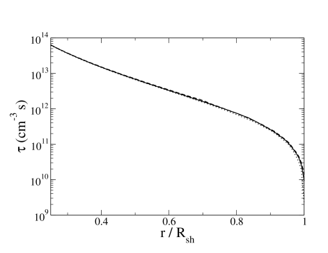
Figure 1.— Ionization timescale parameter $\tau$ (Equation 2) versus radius $r$ scaled to the cluster shock radius $R_{\rm sh}$ for cluster models with total accreted masses of $M_{\rm sh}=0.77$ (dashed line), 1.53 (solid line), and 3.06 (dotted line) $\times$ $10^{15}~{}M_{\odot}$ at a redshift of $z=0$. The shock radii for the three clusters from small to high mass are $R_{\rm sh}=3.31,4.22$, and 5.41 Mpc, respectively. All three lines lie almost on top of one another.

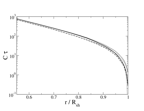
Figure 2.— Dimensionless ionization parameter $C_{i}(T_{e})\tau$ for O VII versus the scaled radius ($r/R_{\rm sh}$) for clusters with total accreted masses of $M_{\rm sh}=0.77$ (dashed line), 1.53 (solid line), and 3.06 (dotted line) $\times$ $10^{15}~{}M_{\odot}$ at a redshift of $z=0$. Models with $\beta=1/1800$ (non-equipartition) and $\beta=1$ (equipartition) are shown in thick and thin lines, respectively.

Figure 3.— Dimensionless ionization parameter $C_{i}(T_{e})\,\tau$ for O VII versus the scaled radius ($r/R_{\rm sh}$) for clusters at different redshifts. The cluster model with a total accreted mass $M_{\rm sh}=1.53\times 10^{15}~{}M_{\odot}$ at $z=0$ is used. Models with $\beta=1/1800$ (non-equipartition) and $\beta=1$ (equipartition) are shown in thick and thin lines, respectively.

Figure 4.— Non-equilibrium ionization bias versus the scaled radius ($r/R_{\rm sh}$) for clusters with total accreted masses of $M_{\rm sh}=0.77$ (dashed line), 1.53 (solid line), and 3.06 (dotted line) $\times$ $10^{15}~{}M_{\odot}$ at a redshift of $z=0$. Models with $\beta=1/1800$ (non-equipartition) and $\beta=1$ (equipartition) are shown in thick and thin lines, respectively.

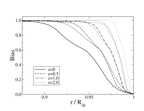
Figure 5.— Non-equilibrium ionization bias versus the scaled radius ($r/R_{\rm sh}$) for clusters at different redshifts. The cluster model with a total accreted mass $M_{\rm sh}=1.53\times 10^{15}~{}M_{\odot}$ at $z=0$ is used. Models with $\beta=1/1800$ (non-equipartition) and $\beta=1$ (equipartition) are shown in thick and thin lines, respectively.

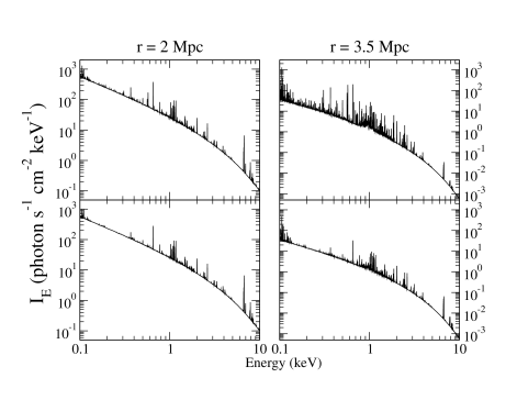
Figure 6.— Projected rest frame spectra for the cluster model with an accreted mass of $M_{\rm sh}=1.53\times 10^{15}~{}M_{\odot}$ at $z=0$ are shown at two projected radii (left: 2 Mpc; right: 3.5 Mpc). Upper panels: the NEI model with $\beta=1/1800$ and non-equipartition of electrons and ions. Lower panels: projected rest frame spectra for the CIE model with the same $\beta$ and non-equipartition.

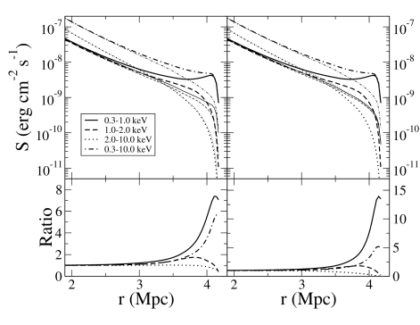
Figure 7.— Upper left panel: rest frame projected surface brightness profiles for different energy bands for the NEI model with $\beta=1/1800$ (thick lines) and the CIE–Non-Eq model (thin lines). Upper right panel: rest frame projected surface brightness profiles for the NEI model with $\beta=1/1800$ (thick lines) and the CIE–Eq model (thin lines). Lower left panel: ratios of the surface brightness profiles $S_{\rm NEI}/S_{\rm CIE-Non{\text{-}}Eq}$. Lower right panel: ratios of the surface brightness profiles $S_{\rm NEI}/S_{\rm CIE-Eq}$.

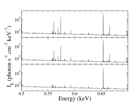
Figure 8.— Upper panel: projected rest frame spectra for the NEI model with $\beta=1/1800$. Middle panel: projected rest frame spectra for the NEI model with $\beta=0.5$. Lower panel: projected rest frame spectra for the CIE–Non-Eq model with $\beta=1/1800$. All spectra are for the $M_{\rm sh}=1.53\times 10^{15}~{}M_{\odot}$ at $z=0$, and are for a projected radius of $r=2$ Mpc. The spectra are binned with $\Delta E=0.1$ eV.

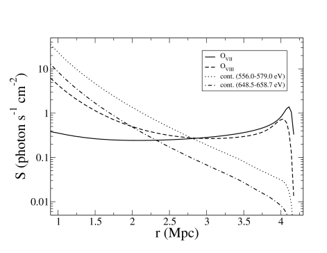
Figure 9.— Surface brightness of the O VII and O VIII lines for the NEI model with $\beta=1/1800$ as a function of projected radius. The continuum emission within the narrow energy bands covering the lines is also shown.

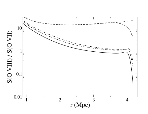
Figure 10.— Line ratios $S($O VIII$)/S($O VII$)$ for the NEI models with $\beta=1/1800$ (solid), 0.5 (dash-dotted), and 1.0 (dash-dot-dotted). Line ratios for the CIE–Non-Eq (dashed) and CIE–Eq (dotted) models are also shown.

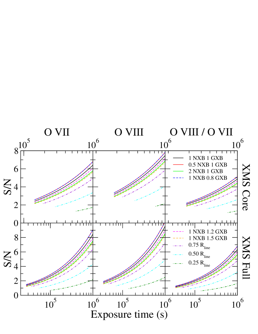
Figure 11.— Left (middle) panels show the signal-to-noise ratios for the O VII triplets (O VIII doublets) expected to be detected by IXO. The right panels show the signal-to-noise ratios for the O VII and O VIII line ratios. The upper panels correspond to the XMSC, and the lower panels correspond to the XMSF. Different signal and noise levels are assumed for the different models. The legends for the lines are the same for all panels, but are separated into two panels due to the space limitation.

References

- Allen et al. (2008) Allen, S. W., Rapetti, D. A., Schmidt, R. W., Ebeling, H., Morris, R. G., & Fabian, A. C. 2008, MNRAS, 383, 879
- Akahori & Yoshikawa (2008) Akahori, T., & Yoshikawa, K. 2008, PASJ, 60, L19
- Akahori & Yoshikawa (2010) Akahori, T., & Yoshikawa, K. 2010, PASJ, 62, 335
- Anders & Grevesse (1989) Anders, E. & Grevesse, N. 1989, Geochim. Cosmochim. Acta, 53, 197
- Basu et al. (2010) Basu, K., et al. 2010, A&A, 519, A29
- Borkowski et al. (2001) Borkowski, K. J., Lyerly, W. J., & Reynolds, S. P. 2001, ApJ, 548, 820
- Borkowski et al. (1994) Borkowski, K. J., Sarazin, C. L., & Blondin, J. M. 1994, ApJ, 429, 710
- Cen & Fang (2006) Cen, R., & Fang, T. 2006, ApJ, 650, 573
- Fang et al. (2005) Fang, T., Croft, R. A. C., Sanders, W. T., Houck, J., Davé, R., Katz, N., Weinberg, D. H., & Hernquist, L. 2005, ApJ, 623, 612
- Fox & Loeb (1997) Fox, D. C., & Loeb, A. 1997, ApJ, 491, 459
- George et al. (2009) George, M. R., Fabian, A. C., Sanders, J. S., Young, A. J., & Russell, H. R. 2009, MNRAS, 395, 657
- Ghavamian et al. (2007) Ghavamian, P., Laming, J. M., & Rakowski, C. E. 2007, ApJ, 654, L69
- Haardt & Madau (1996) Haardt, F., & Madau, P. 1996, ApJ, 461, 20
- Hoshino et al. (2010) Hoshino, A., et al. 2010, PASJ, 62, 371
- Hughes & Helfand (1985) Hughes, J. P., & Helfand, D. J. 1985, ApJ, 291, 544
- Ji et al. (2006) Ji, L., Wang, Q. D., & Kwan, J. 2006, MNRAS, 372, 497
- Kaastra et al. (1996) Kaastra, J. S., Mewe, R., & Nieuwenhuijzen, H. 1996, in UV and X-ray Spectroscopy of Astrophysical and Laboratory Plasmas, ed. K. Yamashita & T. Watanabe (Tokyo: Universal Academy Press), 411
- Komatsu et al. (2010) Komatsu, E., et al. 2010, ApJ, in press (arXiv:1001.4538)
- Kuntz & Snowden (2000) Kuntz, K. D., & Snowden, S. L. 2000, ApJ, 543, 195
- Loeb (2002) Loeb, A. 2002, New Astronomy, 7, 279
- Lueker et al. (2010) Lueker, M., et al. 2010, ApJ, 719, 1045
- Mazzotta et al. (1998) Mazzotta, P., Mazzitelli, G., Colafrancesco, S., & Vittorio, N. 1998, A&AS, 133, 403
- McCammon et al. (2002) McCammon, D., et al. 2002, ApJ, 576, 188
- Raymond & Smith (1977) Raymond, J. C., & Smith, B. W. 1977, ApJS, 35, 419
- Reiprich et al. (2009) Reiprich, T. H., et al. 2009, A&A, 501, 899
- Rudd & Nagai (2009) Rudd, D. H., & Nagai, D. 2009, ApJ, 701, L16
- Sarazin (1986) Sarazin, C. L. 1986, Reviews of Modern Physics, 58, 1
- Smith et al. (2010) Smith, R. K., Bautz, M. W., Bookbinder, J., Garcia, M. R., Guainazzi M., & Kilbourne, C. A. 2010, SPIE, 7732, 773246 (http://ixo.gsfc.nasa.gov/resources/Published_Papers/DOCS/ SPIE_2010/IXO-bkgnd-SPIE.pdf)
- Smith et al. (2001) Smith, R. K., Brickhouse, N. S., Liedahl, D. A., & Raymond, J. C. 2001, ApJ, 556, L91
- Smith & Hughes (2010) Smith, R. K., & Hughes, J. P. 2010, ApJ, 718, 583
- Snowden (1998) Snowden, S. L. 1998, in IAU Colloq. 166: The Local Bubble and Beyond, ed. D. Breitschwerdt, M. J. Freyberg, & J. Truemper (Berlin: Springer), 103
- Takizawa (1999) Takizawa, M. 1999, ApJ, 520, 514
- Takizawa (2000) Takizawa, M. 2000, ApJ, 532, 183
- Verner et al. (1996) Verner, D. A., Ferland, G. J., Korista, K. T., & Yakovlev, D. G. 1996, ApJ, 465, 487
- Vikhlinin et al. (2009) Vikhlinin, A., et al. 2009, ApJ, 692, 1033
- Wechsler et al. (2002) Wechsler, R. H., Bullock, J. S., Primack, J. R., Kravtsov, A. V., & Dekel, A. 2002, ApJ, 568, 52
- Wong & Sarazin (2009) Wong, K.-W., & Sarazin, C. L. 2009, ApJ, 707, 1141
- Wong et al. (2010) Wong, K.-W., Sarazin, C. L., & Wik, D. R. 2010, ApJ, 719, 1
- Yoshikawa & Sasaki (2006) Yoshikawa, K., & Sasaki, S. 2006, PASJ, 58, 641
- Yoshikawa et al. (2003) Yoshikawa, K., Yamasaki, N. Y., Suto, Y., Ohashi, T., Mitsuda, K., Tawara, Y., & Furuzawa, A. 2003, PASJ, 55, 879
- Zhao et al. (2009) Zhao, D. H., Jing, Y. P., Mo, H. J., & Börner, G. 2009, ApJ, 707, 354