On the efficient and accurate short-ranged simulations of uniform polar molecular liquids

Abstract

We show that spherical truncations of the $1/r$ interactions in models for water and acetonitrile yield very accurate results in bulk simulations for all site-site pair correlation functions as well as dipole-dipole correlation functions. This good performance in bulk simulations contrasts with the generally poor results found with the use of such truncations in nonuniform molecular systems. We argue that Local Molecular Field (LMF) theory provides a general theoretical framework that gives the necessary corrections to simple truncations in most nonuniform environments and explains the accuracy of spherical truncations in uniform environments by showing that these corrections are very small. LMF theory is derived from the exact Yvon-Born-Green (YBG) hierarchy by making physically-motivated and well-founded approximations. New and technically interesting derivations of both the YBG hierarchy and LMF theory for a variety of site-site molecular models are presented in appendices. The main paper focuses on understanding the accuracy of these spherical truncations in uniform systems both phenomenologically and quantitatively using LMF theory.

I Introduction

Spherical truncations of the Coulomb interactions present in typical molecular models such as CHARMM MacKerellBashfordBellott.1998.All-Atom-Empirical-Potential-for-Molecular-Modeling ; BrooksBrooksMackerell.2009.CHARMM:-The-Biomolecular-Simulation-Program and AMBER DuanWuChowdhury.2003.A-point-charge-force-field-for-molecular-mechanics have long been used to keep computational cost in check. This cost in the simulation of large biomolecules is compounded by the use of explicit water models containing point charges to describe the hydrogen-bonding network and dielectric behavior of the solvating water molecules. Since traditional particle-mesh Ewald sum treatments of Coulomb interactions do not scale well in massively parallel simulations, a computationally compelling case can be made for the use of spherical truncations Schulz:2009p5308 . However, spherical truncations have been shown to be clearly wrong when applied naively in a variety of nonuniform environments Feller:1996p5303 ; Spohr.1997.Effect-of-Electrostatic-Boundary-Conditions-and-System . For this reason, the use of short-ranged truncations of $1/r$ interactions is typically viewed as an unjustified approximation.

There have been many attempts to place the use of spherical truncations of $1/r$ on a more solid theoretical footing, including site-site reaction field methods HummerSoumpasisNeumann.1994.Computer-simulation-of-aqueous-Na-Cl-Electrolytes , Wolf summation FennellGezelter.2006.Is-the-Ewald-summation-still-necessary-Pairwise ; WolfKeblinskiPhillpot.1999.Exact-method-for-the-simulation-of-Coulombic-systems , and isotropic periodic summation WuBrooks.2005.Isotropic-periodic-sum:-A-method-for-the-calculation ; WuBrooks.2008.Using-the-isotropic-periodic-sum-method-to-calculate ; WuBrooks.2009.Isotropic-periodic-sum-of-electrostatic-interactions-for-polar . Despite this work, the virtues and defects of spherical truncations of $1/r$ in various applications remains a subject of ongoing debate in the current literature Schulz:2009p5308 ; Patra:2003p5327 ; Patra:2004p5329 ; Patra:2006p5332 .

Our approach, local molecular field (LMF) theory ChenKaurWeeks.2004.Connecting-systems-with-short-and-long ; RodgersWeeks.2008.Local-molecular-field-theory-for-the-treatment , uses an effective single particle potential to account for the averaged effects of the long-ranged interactions neglected in typical spherical truncations. It gives a theoretical basis for the use of simple truncations in some cases, and also provides a physically suggestive path for correction when such truncations fail. Moreover, recent work has established a very efficient and accurate numerical method to determine the effective field in LMF theory using a simple linear response approach HuWeeks.2010.Efficient-Solutions-of-Self-Consistent-Mean-Field .

LMF theory for general nonuniform fluids is derived from the exact statistical mechanical Yvon-Born-Green (YBG) hierarchy HansenMcDonald.2006.Theory-of-Simple-Liquids ; McQuarrie.2000.Statistical-Mechanics by making two physically-motivated and well-founded approximations. These rely on the ability of well-chosen truncated potentials to yield accurate nearest-neighbor correlations and on the corresponding slowly-varying nature of the remaining long-ranged parts of the full potential RodgersWeeks.2008.Local-molecular-field-theory-for-the-treatment . Previous work has shown that LMF theory corrects two well known failures of spherical truncations of $1/r$ interactions:

• simulations using LMF theory yield correct charge density profiles for water confined between two walls RodgersWeeks.2008.Interplay-of-local-hydrogen-bonding-and-long-ranged-dipolar and for ions confined between charged plates RodgersKaurChen.2006.Attraction-between-like-charged-walls:-Short-ranged , and

• simple analytical corrections derived via LMF theory result in accurate energies and pressures for uniform ionic and molecular systems ChenKaurWeeks.2004.Connecting-systems-with-short-and-long ; RodgersWeeks.2009.Accurate-thermodynamics-for-short-ranged-truncations-of-Coulomb treated with spherical truncations.

In this paper we employ LMF theory to illustrate and explain why spherical truncations of $1/r$ can often be applied very successfully for determining the structure and thermodynamics of uniform molecular systems. When LMF theory is applied to charge-charge interactions, all $1/r$ interactions are split into short and long ranged parts $v_{0}(r)$ and $v_{1}(r)$, such that

$$\frac{1}{r}=v_{0}(r)+v_{1}(r)\equiv\frac{\operatorname{erfc}(r/\sigma)}{r}+\frac{\operatorname{erf}(r/\sigma)}{r}.$$ (1)

Here $v_{1}(r)$ is the electrostatic potential from a unit Gaussian charge distribution with width $\sigma$, and $v_{0}(r)$ corresponds to the potential from a point charge surrounded by a neutralizing Gaussian charge distribution ChenKaurWeeks.2004.Connecting-systems-with-short-and-long . Thus $v_{0}(r)$ vanishes at distances $r$ much greater than the “smoothing length” $\sigma$ and at small distances the force from $v_{0}(r)$ approaches that of the bare point charge, so $v_{0}(r)$ can be though of as a “Coulomb core potential”.

In the simple strong coupling approximation (SCA) to the full LMF theory, we assume that all effects from the long-ranged interactions due to $v_{1}(r)$ may be neglected. Thus the SCA is in essence a spherical truncation where all $1/r$ interactions are replaced by the short-ranged $v_{0}(r)$, with $\sigma$ setting the scale for the truncation distance. In Section II, we emphasize the accuracy of the SCA for uniform molecular systems, presenting results for SPC/E water and acetonitrile (CH₃CN), including the effect of varying the range of the short-ranged truncation of $1/r$ as represented by $\sigma$ in equation (1). These results can be appreciated independent of the underlying LMF theory discussed in the rest of this paper.

Furthermore, we demonstrate that spherical truncations can lead to highly accurate dipole-dipole correlations in uniform molecular systems. This surprising result is in sharp contrast to findings by Nezbeda, who used a different molecular-based truncation scheme Nezbeda.2005.Towards-a-Unified-View-of-Fluids , and we shall explain our success later using the full LMF theory. Then in Sections III and IV, we formulate LMF theory for bulk uniform site-site molecular fluids and discuss the success of these spherical truncations and the neglect of long-ranged interactions using the LMF theory framework for the simpler bulk water system. The form of the derived LMF equation and the necessary approximations make clear why spherical truncations can often give accurate structure in uniform systems, despite their invalidity in nonuniform systems.

Detailed derivations of LMF equations for various molecular models are discussed in complementary appendices. Here we build on previous derivations of LMF theory for simple atomic fluids, and focus in particular on the derivation of the LMF equation for a uniform system of site-site molecules, described by the Hamiltonian

$${\cal U}=\sum_{i=1}^{N}\omega_{M}(\mathbf{R}_{i})+\frac{1}{2}\sum_{i=1}^{N}\sum_{j=1}^{N}(1-\delta_{ij})\sum_{\alpha=1}^{n}\sum_{\xi=1}^{n}u_{\alpha\xi}(|{\mathbf{r}}_{i}^{(\alpha)}-{\mathbf{r}}^{(\xi)}_{j}|).$$ (2)

Here $\mathbf{R}_{i}$ describes the positions of all sites within a molecule $i$ connected by a generalized bonding potential $\omega_{M}(\mathbf{R}_{i})$, and $u_{\alpha\xi}(|{\mathbf{r}}_{i}^{(\alpha)}-{\mathbf{r}}^{(\xi)}_{j}|)$ describes the general pair interaction between two sites $\alpha$ and $\xi$ on two different molecules $i$ and $j$ as insured by the $\delta_{ij}$ term in equation (2). In Appendix A, we present a derivation of the LMF equation used in previous work for small site-site molecules in a general external field. Then in Appendices B and C, we present the notationally more complex derivations of both the exact YBG hierarchy and the LMF equation for a uniform fluid composed of these site-site molecules. Finally, in Appendix D, we present an abbreviated derivation for larger molecules described by CHARMM- or AMBER-like Hamiltonians, thus supporting the validity of our conclusions for systems composed of much larger molecules.

II Strong Coupling Approximation (SCA) Simulations of Water and Acetonitrile

We present structural results for the simulation of two different small site-site molecular models shown in Fig. 1:

• SPC/E water BerendsenGrigeraStraatsma.1987.The-missing-term-in-effective-pair-potentials , a rigid molecular model of a hydrogen-bonding fluid, and

• acetonitrile, an AMBER-like flexible molecular model NikitinLyubartsev.2007.New-six-site-acetonitrile-model-for-simulations-of-liquid of a strongly dipolar fluid.

These models, along with annotation used for each site, are shown in Fig. 1.

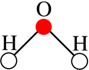
(a) SPC/E Water

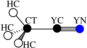
(b) Acetonitrile

Figure 1: Schematics depicting the geometry and site labels of the water model BerendsenGrigeraStraatsma.1987.The-missing-term-in-effective-pair-potentials and acetonitrile model NikitinLyubartsev.2007.New-six-site-acetonitrile-model-for-simulations-of-liquid used in this paper.

For the water simulations, we present results for simulations of 1728 SPC/E water molecules in a cubic box of side length 37.27 Å using the dlpoly2.16 simulation package SmithYongRodger.2002.DLPOLY:-Application-to-molecular-simulation . The system of water molecules was equilibrated for 500 ps at 300 K using a Berendsen thermostat with a time constant of 0.5 ps and a timestep of 1 fs. Data was collected over the subsequent 1.5 ns. Cutoff radii for the potential ranged from 9.5 Å up to 13.5 Å for varying choices of $\sigma$ in $v_{0}(r)$. The SCA simulations are compared to simulations using Ewald summation with $\alpha=0.3$ Å^-1 and $\mathbf{k}_{\rm max}=(10,10,10)$.

We have previously shown that the SCA with a $\sigma$ of 4.5 Å gives a highly accurate O-O pair correlation function for SPC/E water RodgersWeeks.2008.Interplay-of-local-hydrogen-bonding-and-long-ranged-dipolar . In Fig. 2(a-c), we show the pair correlation functions for all site-site pairs using the SCA with $\sigma$ ranging from 3.0 Å to 6.0 Å. In all instances, the $g(r)$ are in excellent agreement with results of the full system determined using Ewald sums. In the plot of $g_{\rm HH}(r)$, the curves for each $\sigma$ choice are displaced by 0.2 in order to emphasize that all plots contain multiple choices of $v_{0}(r)$ while yielding essentially the same correlation functions on the scale of the graph.

These data illustrate the important point that $\sigma$ is a consistency parameter rather than an empirical fitting parameter ChenKaurWeeks.2004.Connecting-systems-with-short-and-long ; RodgersWeeks.2008.Local-molecular-field-theory-for-the-treatment . Thus the mean field averaging leading to LMF theory become highly accurate for any choice of $\sigma$ greater than a state dependent minimum value $\sigma_{\text{min}}$, typically of order a characteristic nearest neighbor distance. For SPC/E water $\sigma_{\text{min}}$ is about $3~{}\AA$, the radius of the Lennard-Jones (LJ) core on the water molecule. Any smaller $\sigma$ would clearly yield a short-ranged system that does not accurately describe the oxygen-hydrogen charge correlations on neighboring molecules that compete with the LJ core repulsions in forming hydrogen bonds, and indeed poor agreement is found at smaller $\sigma$.

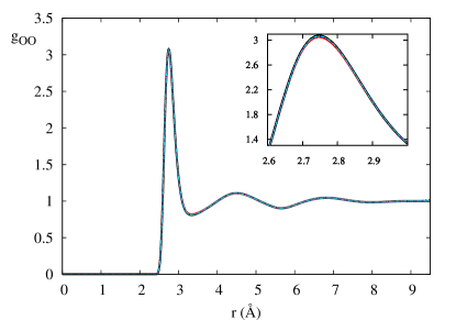
(a) $g_{\rm OO}(r)$

(b) $g_{\rm OH}(r)$

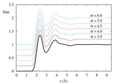
(c) $g_{\rm HH}(r)$

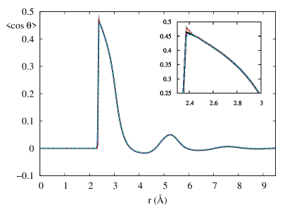
(d) $\left<\cos\theta\right>(r)$

Figure 2: $g(r)$ for each site-site pair of SPC/E water, as well as $\left<\cos\theta\right>(r)$. All plots display the correlations determined via both Ewald summation (Full) and spherical truncation via LMF theory. The smoothing length $\sigma$ ranges from 3.0 Å to 6.0 Å in all plots. In the plot of $g_{\rm HH}(r)$, the curves for each $\sigma$ choice are displaced by 0.2 in order to emphasize that all plots shown contain multiple choices of $v_{0}(r)$. Insets in (a) and (d) focus on the region near the peak height, where small errors in the $\sigma=3.0~{}\AA\$ curves are just visible.

We also carried out molecular dynamics simulations of bulk acetonitrile at two very different states, a high density liquid very near liquid-vapor coexistence at 298 K and a lower density system at 550 K. We used a six-site model with flexible bonds developed by Nikitin and Lyubartsev NikitinLyubartsev.2007.New-six-site-acetonitrile-model-for-simulations-of-liquid in which intermolecular potential parameters have been optimized for better consistency with experiments. In order to simulate at appropriate bulk densities, an initial configuration of 864 molecules in a cubic box is equilibrated for several hundred picoseconds (ps) in the NPT ensemble using the Nose-Hoover thermostat and barostat until the volume has equilibrated. The low temperature system has a simulation box length of 42.2 Å. The dilute system at 550 K has a density one-third that of 298 K and is further equilibrated in the NVT ensemble for several hundred picoseconds. The cutoffs of the Lennard-Jones interactions were set to 15 Å. When the SCA is employed, the cutoffs for $v_{0}(r)$ were 15 Å for $\sigma=4.5$ Å, 21 Å for $\sigma=6.5$ Å, and 30 Å for $\sigma=8.5$ Å. When Ewald summation was employed as a benchmark, the cutoff for the real space interactions was set to 15 Å, and $\alpha=0.26$ Å^-1 with $\mathbf{k}_{\rm max}=(15,15,15)$.

Results for acetonitrile site-site pair correlation functions are shown in Figs. 3 and 4. These figures focus on the pair correlations at both 298 K and 550 K between a nitrogen site (YN) and all four molecular sites on another molecule. The remaining six intermolecular site-site pair correlations are described just as accurately, and are not displayed for brevity. For the high density room temperature system, both $\sigma$ shown yield quite accurate results. Note that the $\sigma$ values are comparable to those used for water, despite the greater size of the acetonitrile molecule. Very poor results (not shown) were obtained with use of a too small $\sigma=2.5$ Å as would be expected.

For the higher temperature, lower density system, $\sigma=4.5$ Å performs poorly and is not shown, $\sigma=6.5$ Å is markedly improved, and only the largest $\sigma$ of 8.5 Å yields high quality agreement with the Ewald simulation. This is expected from simple scaling arguments since the typical nearest neighbor distance is larger; multiplying $\sigma_{\rm min}=4.5$ Å for 298 K by the requisite increase in interparticle spacing at lower densities yields 6.5 Å. The need for a somewhat larger $\sigma_{\rm min}$ is likely a result of the increasing relevance of more extended conformations of these molecules at lower densities and higher temperatures. Both the water and acetonitrile results show that spherical truncations are quite good in bulk fluids, given a sufficiently large truncation radius. This is phenomenologically well established in the literature.

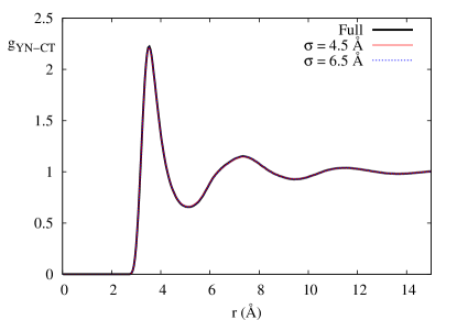
(a) $g_{\rm YN-CT}(r)$

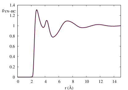
(b) $g_{\rm YN-HC}(r)$

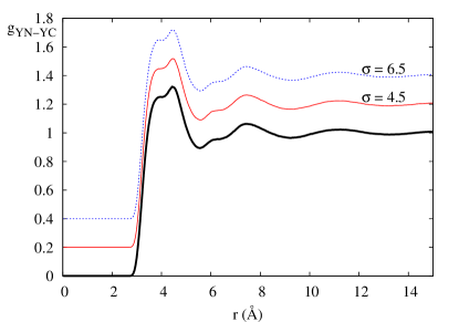
(c) $g_{\rm YN-YC}(r)$

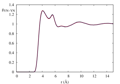
(d) $g_{\rm YN-YN}(r)$

Figure 3: Pair correlation functions for the nitrogen site YN on acetonitrile at 298 K as $\sigma$ varies from 4.5 Å to 6.5 Å. As before, the plot of $g_{\rm YN-YC}(r)$ displays the $g(r)$ displaced by 0.2 but all plots display results for Ewald summation (Full) and all choices of $\sigma$.

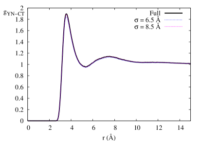
(a) $g_{\rm YN-CT}(r)$

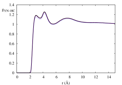
(b) $g_{\rm YN-HC}(r)$

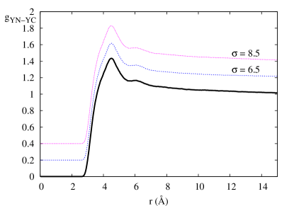
(c) $g_{\rm YN-YC}(r)$

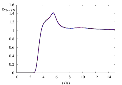
(d) $g_{\rm YN-YN}(r)$

Figure 4: Pair correlation functions for the nitrogen site YN on acetonitrile at 550 K as $\sigma$ varies from 6.5 Å to 8.5 Å. As before, the plot of $g_{\rm YN-YC}(r)$ displays the $g(r)$ displaced by 0.2 but all plots display results for Ewald summation (Full) and all choices of $\sigma$.

The strong agreement of all the acetonitrile site-site correlation functions, given a sufficiently large $\sigma$, suggests that the angular correlations between these molecules are also accurate, for otherwise many of the unusual functional forms would not be reproduced with fidelity. Thus we also examine angular correlations for both water and acetonitrile.

Fig. 2(d) shows the excellent agreement of dipole-dipole correlations in SPC/E water simulated using the SCA with those correlations in the full Ewald simulations. Here we plot the average $\cos\theta$ between water dipoles as a function of separation distance $r$ between the centers of mass of two water molecules. Such good agreement is not a consequence of the relatively compact nature of the water molecule. Shown in Fig. 5 are plots of $\left<\cos\theta\right>(r)$ for the acetonitrile system at each temperature. We again find quite good agreement between the angular correlations in the full Ewald system and our short-ranged systems. This agreement follows the trends found for the simpler site-site distribution functions, with a larger $\sigma$ needed for the low density higher temperature state.

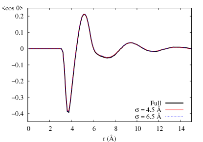
(a) $T=298$ K

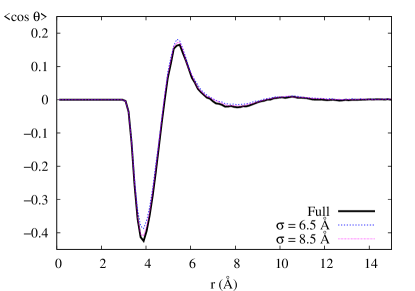
(b) $T=550$ K

Figure 5: Angular correlations represented by $\left<\cos\theta\right>(r)$ for acetonitrile at 298 K (left) and 550 K (right) as $\sigma$ varies.

We believe that the excellent agreement of the dipole-dipole correlations in these spherically truncated fluids is a direct consequence of the general validity of LMF theory and the accuracy of the strong coupling approximation in uniform environments, as we describe in the following section. Nezbeda has previously reported poor results for dipole-dipole correlations in short-ranged systems where the determined $g(r)$ were accurate Nezbeda.2005.Towards-a-Unified-View-of-Fluids . The crux of the difficulties with his chosen cutoff scheme was defining these cutoffs on a molecular basis, rather than a site basis. This leads to neglected potentials which actually rapidly vary near the cutoff radius, counter to one of the important assumptions of LMF theory as discussed in the next section. Takahashi and coworkers TakahashiNarumiYasuoka.2010.Cutoff-radius-effect-of-the-isotropic-periodic studied the effect of cutoff radii in the isotropic periodic sum approach on various properties of water and found for $\left<\cos\theta\right>(r)$ that deviations in this property were minimal and equivalent for cutoff radii greater than 16 Å. This cutoff radius for IPS can be compared to the cutoff radius of 13.5 Å used for $\sigma=6.0$ Å in this paper. We take their observed “saturation” in errors beyond a given cutoff radius as an indication that their spherically-truncated potential satisfies the necessary conditions for the validity of LMF theory.

III Local Molecular Field (LMF) Theory for Site-Site Molecules

LMF theory for a general nonuniform system prescribes a mapping from the system of interest where all particles interact via their full intermolecular potentials in the presence of an external field to a “mimic system” where particles interact via short-ranged truncations of their intermolecular potentials but in the presence of a an effective or restructured field. The restructured field accounts for the effects of the long-ranged components of the intermolecular interactions using a mean field average. Far from being a simplistic mean-field ansatz, LMF theory has been shown to be strongly rooted in statistical mechanical theory, and based on physically-motivated approximations that are well-justified for dense fluid systems.

LMF theory for charged systems takes a particularly simple form when charges alone are treated via LMF theory using a single $\sigma$, where the results can be exactly re-expressed in terms of the total charge density and a restructured electrostatic potential. Based on the splitting of $1/r$ defined in equation (1), each pair potential $u_{\alpha\xi}(r)$ in equation (2) may be decomposed as

$$u_{\alpha\xi}(r)=u_{0,\alpha\xi}(r)+\frac{q_{\alpha}q_{\xi}}{\epsilon}v_{1}(r),$$ (3)

where $u_{0,\alpha\xi}(r)$ contains all the non-electrostatic Lennard-Jones-like pair interactions as well as a $v_{0}(r)$ contribution appropriately scaled by charge and the dielectric constant $\epsilon$. The crucial feature of these two potentials $v_{0}(r)$ and $v_{1}(r)$ for the validity of LMF theory is that $\sigma$ is chosen so that $v_{0}(r)$ contains all relevant strong Coulomb forces between nearest neighbors and that $v_{1}(r)$ is consequently slowly-varying over the range of strongest correlations between those neighbors. A more careful statement of the relevant approximations may be found in Appendix A.

Previous work focused on nonuniformity such as confining walls, using the Coulomb LMF equation  RodgersWeeks.2008.Interplay-of-local-hydrogen-bonding-and-long-ranged-dipolar ; RodgersWeeks.2008.Local-molecular-field-theory-for-the-treatment

$$\mathcal{V}_{R}(\mathbf{r})=\mathcal{V}_{0}(\mathbf{r})+\frac{1}{\epsilon}\int d\mathbf{r}^{\prime}\,\rho^{q}_{R,\text{tot}}(\mathbf{r}^{\prime})v_{1}\left(\left|\mathbf{r}-\mathbf{r^{\prime}}\right|\right),$$ (4)

where $\mathcal{V}_{0}$ results from the convolution of the fixed charge density with $v_{0}(r)$, and $\rho^{q}_{R,\text{tot}}$ includes both the fixed and mobile charge densities. Note that $\mathcal{V}_{R}$ and $\rho^{q}_{R,\text{tot}}$ are implicitly functionals of one another, so this is a self-consistent equation.

Since $v_{1}(r)$ is the electrostatic potential arising from a Gaussian charge density with width $\sigma$, equation (4) suggests that the restructured external potential $\mathcal{V}_{R}$ may be understood as an electrostatic potential containing the full impact of fixed charges and the Gaussian-smoothed impact of mobile charges. In Appendix A, we present a derivation of the LMF equation for site-site molecular models as used in previous papers. Equation (4) is identical to that for mixtures of charged species RodgersWeeks.2008.Local-molecular-field-theory-for-the-treatment , and a derivation for small site-site molecular models requires only one further approximation, requiring that intramolecular correlations are well represented by the mimic system, a seemingly very reasonable requirement. The solution of equation (4) has been shown to yield accurate structure for both ionic solutions ChenWeeks.2006.Local-molecular-field-theory-for-effective ; RodgersKaurChen.2006.Attraction-between-like-charged-walls:-Short-ranged and molecular water RodgersWeeks.2008.Interplay-of-local-hydrogen-bonding-and-long-ranged-dipolar in nonuniform systems, and a simple linear response method for solving the above equation has been derived HuWeeks.2010.Efficient-Solutions-of-Self-Consistent-Mean-Field , leading to fast and computationally efficient solutions of the LMF equation.

Site-site pair correlations in bulk fluids may be simply related to those arising from fixing a given site at the origin, thus allowing us to describe structure in uniform fluids from the nonuniform perspective of LMF theory in equation (4). As such, for bulk molecular fluids with spherically symmetric site-site interactions as considered here, we would expect that the general LMF equation (4) in this case could then be written as

$${\mathcal{V}_{R|\eta}}(r)=\frac{q_{\eta}}{\epsilon}v_{0}(r)+\frac{1}{\epsilon}\int d\mathbf{r}^{\prime}\,\rho_{R,\text{tot}}^{q}({r^{\prime}|{\mathbf{0}}})v_{1}\left(\left|\mathbf{r}-\mathbf{r^{\prime}}\right|\right),$$ (5)

with $\eta$ being the site fixed at the origin as indicated by the conditional notation $|\eta$ on the left side of equation (5). In analogy with equation (4), the first term is the short-ranged potential due to the only fixed charge in the system, the charge from site $\eta$ at the origin. The charge density $\rho_{R,\text{tot}}^{q}(r^{\prime}|{\mathbf{0}})$ is the total charge density in the nonuniform mimic system with $|{\mathbf{0}}$ again indicating the fixed site. In the case of these small site-site molecules, this total charge density may be decomposed as

• the intramolecular charge density arranged around the molecular site $\eta$ fixed at the origin including the site $\eta$, denoted $\varrho^{q}_{R,M|\eta}({r}|{\mathbf{0}})$, and

• the intermolecular charge density from other unconstrained mobile molecules induced by $\eta$, denoted $\rho^{q}_{R}(r|{\mathbf{0}})$.

While only $\eta$ contributes to the $\mathcal{V}_{0}$ in this equation, the intramolecular sites attached to the site $\eta$ fixed at the origin contribute directly to the total charge density $\rho_{R,\text{tot}}^{q}$ and also implicitly but strongly impact the form of the intermolecular charge density $\rho^{q}_{R}$ based on their inclusion in the simulation of the mimic system.

While the discussion above should make the form of equation (5) quite plausible, two further approximations are needed in addition to the three stated in Appendix A to carefully separate effects of intra- and intermolecular charges in this equation and to assess its accuracy for site-site molecular models. Again, we employ the exact relationship between the pair distribution functions in a uniform fluid and the conditional singlet density profile due to a site fixed at the origin.

The YBG hierarchy for site-site molecular systems with one site of one molecule fixed at the origin is derived in Appendix B. The derivation is quite interesting technically, since we use an external field to localize only a particular molecular site at the origin rather than to represent an entire fixed molecule, as is usually done. Moreover, we derive first the YBG hierarchy for correlation functions between specific molecules rather than the usual generic correlation functions used in standard treatments. These features allows us to more easily disentangle contributions from intra- and intermolecular correlation functions. Using this new YBG hierarchy, the derivation of LMF theory for a uniform fluid of site-site molecules then follows the traditional route, while requiring two new but very plausible approximations related to intramolecular correlations, as shown in Appendix C. This provides a rigorous derivation of equation (5).

Towards the goal of understanding the accuracy of SCA truncations in uniform fluids, we rewrite equation (5) in a way that focuses on the long-ranged contributions to $\mathcal{V}_{R}$, which we call $\mathcal{V}_{R1}$:

$${\mathcal{V}_{R1|\eta}}(r)\equiv\mathcal{V}_{R|\eta}(r)-\frac{q_{\eta}}{\epsilon}v_{0}(r)=\frac{1}{\epsilon}\int d\mathbf{r}^{\prime}\,\rho_{R,\text{tot}}^{q}({r^{\prime}|{\mathbf{0}}})v_{1}\left(\left|\mathbf{r}-\mathbf{r^{\prime}}\right|\right).$$ (6)

If $\mathcal{V}_{R1|\eta}\approx 0$ then simulating with spherical truncations alone as in the SCA will give very accurate results.

This $\mathcal{V}_{R1|\eta}$ defined in equation (6) is seen to be the Gaussian-smoothed electrostatic potential arising from the total charge density in the fluid induced by the charge from fixed site $\eta$. This total charge density includes the single molecule charge distribution $\varrho^{q}_{R,M|\eta}({r}|{\mathbf{0}})$ as well as contributions from other fully mobile molecules. As discussed in Refs. RodgersWeeks.2008.Local-molecular-field-theory-for-the-treatment , RodgersWeeks.2008.Interplay-of-local-hydrogen-bonding-and-long-ranged-dipolar , and ChenWeeks.2006.Local-molecular-field-theory-for-effective , the restructured electrostatic potential $\mathcal{V}_{R1}(\mathbf{r})$ induced by a general fixed charge distribution $\rho^{q}_{\rm ext}(\mathbf{r}^{\prime})$ satisfies the single Coulomb LMF equation given by the convolution of $v_{1}(r)$ with $\rho^{q}_{R,\text{tot}}(\mathbf{r}^{\prime})$, including contributions from both fixed and mobile charges, so equation (6) has exactly the form that would be expected.

IV Success of SCA Explained

We specifically explore the meaning and consequences of the LMF equation for SPC/E water, both because it has fewer sites than acetonitrile and also because it has a fixed geometry, thereby allowing for analytical determination of $\varrho^{q}_{R,M|\eta}({r}|{\mathbf{0}})$ without simulation and independent of perturbations from other mobile molecules. For either hydrogen site,

$$\varrho^{q}_{R,M|H}(r|{\mathbf{0}})=q_{H}\delta\left(\mathbf{r}\right)+q_{O}\frac{\delta\left(r-r_{\rm OH}\right)}{4\pi r_{\rm OH}^{2}}+q_{H}\frac{\delta\left(r-r_{\rm HH}\right)}{4\pi r_{\rm HH}^{2}},$$ (7)

and for the oxygen site,

$$\varrho^{q}_{R,M|O}(r|{\mathbf{0}})=q_{O}\delta\left(\mathbf{r}\right)+2q_{H}\frac{\delta\left(r-r_{\rm OH}\right)}{4\pi r_{\rm OH}^{2}},$$ (8)

where the charge densities have been spherically averaged about the site fixed at the origin. Separating out the contribution of these intramolecular charge densities, the total ${\mathcal{V}_{R1|\eta}}$ in equation (6) may be decomposed into intramolecular and intermolecular contributions as

$${\mathcal{V}_{R1|\eta}}(r)=\frac{1}{\epsilon}\int d\mathbf{r}^{\prime}\,\varrho_{R,M|\eta}^{q}({r^{\prime}|{\mathbf{0}}})v_{1}\left(\left|\mathbf{r}-\mathbf{r^{\prime}}\right|\right)+\frac{1}{\epsilon}\int d\mathbf{r}^{\prime}\,\rho_{R}^{q}({r^{\prime}|{\mathbf{0}}})v_{1}\left(\left|\mathbf{r}-\mathbf{r^{\prime}}\right|\right),$$ (9)

where the first term corresponds to the long-ranged interactions due to sites within the molecule with site $\eta$ at the origin.

The success of SCA shown in Section II suggests that $\mathcal{V}_{R1|\eta}\approx 0$ is a well-founded approximation. Before utilizing the analytical charge densities above, we first explore an alternate formulation of LMF theory for site-site molecules which might seem initially fruitful. Theoretical treatments of molecular models often involve fixing a given molecular orientation and considering the fluid response to this configuration. Based on the splitting of $1/r$, the majority of the strong electrostatic potential energy and force will be included in the $v_{0}(r)$ used as a pair potential in SCA simulations. However, for any one orientation of a water molecule, the combined forces due to the $v_{1}(r)$ on other oxygen and hydrogen sites will not be negligible, even though they are slowly-varying on the scale of $\sigma$ for each individual site.

As one example of this, the long-ranged electrostatic potential arising from a fixed orientation of a water molecule with O at the origin and the $1/r$ interactions replaced by $v_{1}(r)$ with $\sigma=4.5$ Å is shown in Fig. 6. Based on this single snapshot of the $v_{1}(r)$ contributions due to intramolecular sites, neglect of these long-ranged forces in the SCA would seem an ill-conceived approximation, and we might suppose that a $\mathcal{V}_{R}$ depending on both intermolecular distance and relative molecular orientations would be required. However, looking at an individual orientation of the water molecule for long-ranged interactions fixes all three intramolecular charges and would be expected to generate a very different and larger density response than the single fixed molecular charge at the origin needed to determine radially-symmetric site-site correlation functions, as the LMF equation (9) and Appendices B and C show.

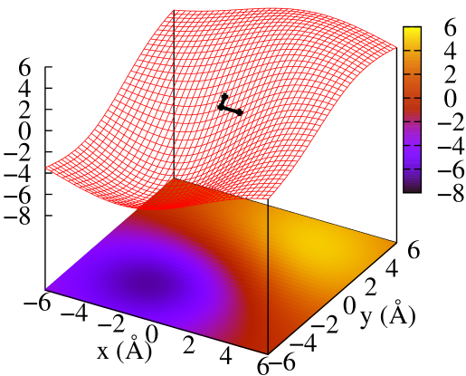
Figure 6: The long-ranged potential in the z=0 plane resulting from a fixed orientation of a water molecule with $\mathbf{r}_{\rm O}=(0,0,0)$, $\mathbf{r}_{\rm H1}=(1,0,0)$, and $\mathbf{r}_{\rm H2}=(-0.334,0.943,0)$ and $\sigma$ chosen as 4.5 Å. The potential is displayed in units of $k_{B}T/e_{0}$ in order to aid in gauging the magnitude of this potential relative to thermal fluctuations. The chosen orientation of the water molecule is shown with solid black lines and points.

The first term in equation (9) may be determined analytically for SPC/E water, and this is the first crucial step in understanding why the full $\mathcal{V}_{R1|\eta}$ will be small to good approximation in uniform systems. As shown in Fig. 7, the spherically symmetric long-ranged potential from the first term, which we shall term $\mathcal{V}_{R1,{\rm intra}|\eta}(r)$ is indeed much more slowly-varying than the orientation-dependent potential shown in Fig. 6. In this figure, we compare $\mathcal{V}_{R1,{\rm intra}|\eta}(r)$ to both the $v_{0}(r)$ due to either O or H fixed at the origin as well as the $v_{1}(r)$ due simply to that site $\eta$.

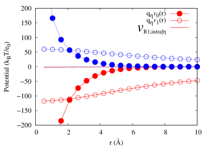
(a) Large Scale

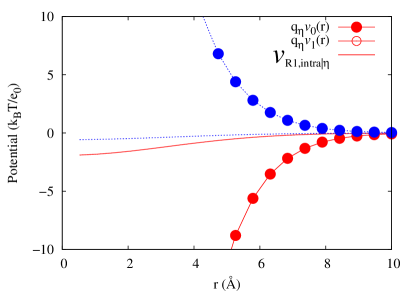
(b) Focus on $\mathcal{V}_{R1,{\rm intra}|\eta}$

Figure 7: Comparison of $\mathcal{V}_{R1,{\rm intra}|\eta}(r)$ to relevant potentials due solely to the site $\eta$ fixed at the origin, whether it be oxygen (red) or hydrogen (blue). This electrostatic potential due to the whole neutral molecule is substantially smaller than both the short-ranged and long-ranged components of $1/r$ due to the individual site fixed at the origin.

From these plots, we see that $\mathcal{V}_{R1,{\rm intra}|\eta}$ is substantially smaller in magnitude than either the electrostatic potential arising from a specific water molecular orientation or the potential due simply to the charge at the site $\eta$ we have fixed at the origin. Therefore, we infer that the spherical truncations prescribed by LMF theory and the associated mean-field averaging of long-ranged interactions will actually be even more effective in bulk molecular simulations than in a corresponding simulation of an ionic system with charges not bound into neutral molecules. Again we emphasize that this spherical averaging is not an unfounded approximation, but that it arises rigorously from the statistical mechanics of molecular models interacting via site-site potentials.

The total electrostatic potential arising from the spherically-averaged intramolecular charge density will be exactly zero for all $r>l_{\rm OH}$ if oxygen is fixed at the origin or for all $r>l_{\rm HH}$ if hydrogen is fixed at the origin. Thus it might seem counterintuitive that the corresponding $\mathcal{V}_{R1,{\rm intra}|\eta}$ is small but non-vanishing beyond this distance. However, the distinct treatments of the short-ranged and long-ranged parts of $1/r$ using Gaussian convolutions in LMF theory require just such a nonzero potential. All the short-ranged parts of $1/r$ are treated explicitly via $v_{0}(r)$ positioned around each site in the water molecule in order to represent local correlations; the capture of these local correlations in the SCA simulation is crucial. In tandem, only the long-ranged components $v_{1}(r)$ are spherically averaged about the fixed site $\eta$ in LMF theory, leading to a non-zero but slowly-varying and small magnitude potential $\mathcal{V}_{R1,{\rm intra}|\eta}(r)$ outside the total potential cutoff. For the correlations between molecules, the need for non-zero short-ranged site-site $v_{0}$ terms seems quite natural; the need for similar short-ranged terms also holds for the far-less intuitively-obvious splitting of the (exactly zero) electrostatic potential between two charged plates ChenWeeks.2006.Local-molecular-field-theory-for-effective .

As demonstrated in Fig. 7, $\mathcal{V}_{R1,{\rm intra}|\eta}(r)$ is quite small and slowly-varying for SPC/E water. However, while this may make the approximation that the total $\mathcal{V}_{R1|\eta}(r)\approx 0$ in equation (9) plausible, it certainly does not guarantee it. Therefore, we also estimate $\mathcal{V}_{R1|\eta}(r)$ by directly inserting the charge density resulting from the Ewald simulation into the LMF equation. The sole care we take is in enforcing overall charge neutrality at the cutoff radius for the potential, as this is also the furthest radius at which $g(r)$ is calculated. As seen in Fig. 8, these potentials are also quite slowly-varying, lending strong credence to the approximation $\mathcal{V}_{R1|\eta}\approx 0$ in determining structure.

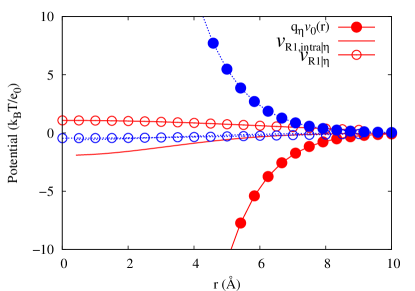
Figure 8: Estimation of $\mathcal{V}_{R1|\eta}$ based on charge densities from the simulations conducted using Ewald summation.

This approach for determining $\mathcal{V}_{R1|\eta}(r)$ requires a full Ewald simulation, contrary to the general philosophy of LMF theory, which seeks to use simulations only in the mimic system. Thus strictly speaking we should self-consistently solve for $\mathcal{V}_{R1|\eta}$ based on charge densities from the short-ranged mimic system using the linear-response treatment developed in Ref. HuWeeks.2010.Efficient-Solutions-of-Self-Consistent-Mean-Field . But previous work has shown that the full LMF theory gives excellent agreement with the results of Ewald simulations for water even in nonuniform environments, so this Ewald determination should be very accurate. Furthermore, care should be exercised with the $k=0$ component of any charge density used in the LMF equation ChenKaurWeeks.2004.Connecting-systems-with-short-and-long ; Rodgers.2008.Statistical-Mechanical-Theory-for-and-Simulations-of-Charged . However, charge densities obtained via Ewald summation exhibit exponential screening and strictly enforce overall neutrality, thus easing the need for great caution in the treatment of the $k=0$ component.

This simple estimate based on the Ewald charge density certainly suffices to demonstrate that $\mathcal{V}_{R1|\eta}(r)$ is small and slowly-varying in this case, and provides strong justification for the accuracy of the SCA. In general we expect that quick estimates of $\mathcal{V}_{R}$ using Ewald charge densities when such simulations are computationally practical will be very useful in obtaining an accurate initial estimate of the final self-consistent $\mathcal{V}_{R}$, and one that will be almost certainly in the linear regime where the method of Ref. HuWeeks.2010.Efficient-Solutions-of-Self-Consistent-Mean-Field will be especially easy to use.

However, for these bulk fluids an accurate $\mathcal{V}_{R1}$ is neither necessary for determining the structure to the accuracy shown here nor for determining the thermodynamics of the fluid as shown in Ref. RodgersWeeks.2009.Accurate-thermodynamics-for-short-ranged-truncations-of-Coulomb . Provided that a sufficiently large $\sigma$ is chosen, simple spherical truncations in simulations coupled with thermodynamic perturbation theory yield accurate structure, energies, and pressures. In the case of SPC/E water, structure might indicate that any $\sigma\geq 3.0$ Å is sufficiently large, but thermodynamics via perturbation theory showed that $\sigma\geq 4.0$ Å is required RodgersWeeks.2009.Accurate-thermodynamics-for-short-ranged-truncations-of-Coulomb .

In general, the choice of a sufficiently large $\sigma$ is crucial for the accuracy of LMF theory. For the acetonitrile system at the higher temperature and lower density, inclusion of a self-consistent $\mathcal{V}_{R1}$ with $\sigma=4.5$ Å gives a poor description of the structure of the acetonitrile system. However, since our simple scaling analysis suggests that $\sigma_{\rm min}\approx 6.5$ Å, we do not expect LMF theory with the smaller $\sigma$ to be able to correct this structure. For the acetonitrile systems at low and high temperature, just as for the water system at ambient temperatures, a sufficiently large $\sigma$ yielded accurate results simply via SCA. Furthermore, the acetonitrile results already demonstrate that $\sigma$ does not need to be on the scale of the entire molecule but rather on the scale of nearest neighbor correlations, as is expected from derivations of LMF theory. In Appendix D, we discuss LMF theory for CHARMM-like molecules in order to better state the necessary conditions for choice of $\sigma$ in much larger molecules.

V Conclusions

In this paper, we have demonstrated the accurate results possible using spherical truncations of $1/r$ interactions in simulations of uniform fluids. We show that these spherical truncations yield not only highly accurate pair correlation functions but also highly accurate dipole-dipole correlation functions. This good performance in bulk simulations of pair correlation functions was known; however, a solid theoretical justification for the use of such spherical truncations in molecular systems has been lacking. In this paper, we present just such a theoretical backing – local molecular field theory. The derivations relevant to LMF theory for a variety of site-site molecular models are presented in appendices and the main paper focuses on understanding the accuracy of these spherical truncations both phenomenologically and quantitatively using LMF theory. LMF theory provides a general conceptual framework that helps us understand why spherical truncations generally work so well in uniform systems and also provides the essential corrections needed in most nonuniform environments.

Appendix A Yvon-Born-Green (YBG) Equation and Local Molecular Field (LMF) Theory Derived for Small Site-Site Molecules in an External Field

While this paper primarily deals with a uniform site-site molecular fluid, the derivations of both the YBG hierarchy as well as the LMF equation are simpler for a general nonuniform system. We present this derivation here using a straightforward method that also introduces the basic site-site notation and ideas that we will then generalize and apply to the uniform fluid in Appendices B and C, where careful attention is paid to the distinction between intra- and intermolecular correlations. We should note that Mullinax and Noid Mullinax:2009p4696 have developed a basis expansion method that can be used to derive a generalized YBG equation for a variety of molecular systems.

Previous work TaylorLipson.1994.A-Site-Site-Born-Green-Yvon-Equation-for-Hard-Sphere for site-site YBG equations begins the derivation by writing the singlet density for a molecular site in terms of the singlet density for the entire molecule with a fixed orientation, taking appropriate gradients on either side, and only then reducing to a site-site representation. Using the general formalism developed by Chandler and Pratt ChandlerPratt.1976.Statistical-Mechanics-of-Chemical-Equilibria-and-Intramolecular for the partition functions and density distribution functions of mixtures of site-site molecular models, we may follow a similar path to the derivation of a general site-site YBG equation. The formalism originally was developed to also account for the possibility of chemical reactions, and since this is not a concern in the inherently classical systems we study, a few alterations will be made to simplify notation, with no impact on the meaning of the equations.

The partition function for a mixture of molecular species $M$ with total sites $n_{M}$ on each molecule labeled by Greek characters such as $\xi$ is given below with the position of the $\xi$ site on the $i^{\rm th}$ molecule of type $M$ given as $\mathbf{r}_{iM}^{(\xi)}$ and the positions of all $n_{M}$ sites on the $i^{\rm th}$ molecule of type $M$ given as $\mathbf{R_{iM}}$.

$$Q(\{M\})=\left(\prod_{M}N_{M}!\nu_{M}^{N_{M}}\prod_{\xi=1}^{n_{M}}\left(\Lambda_{M}^{(\xi)}\right)^{3N_{M}}\right)^{-1}\int\,e^{-\beta\mathcal{U}}\,\left(\prod_{M,i}d\mathbf{R_{iM}}\right)$$ (10)

where the total potential energy $\mathcal{U}$ is defined as

$$\mathcal{U}=\sum_{M}\sum_{i=1}^{N_{M}}\omega_{M}(\mathbf{R_{iM}})+\sum_{M}\sum_{i=1}^{N_{M}}\sum_{\xi=1}^{n_{M}}\phi_{M,\xi}(\mathbf{r_{iM}^{(\xi)}})$$

$$\qquad+\frac{1}{2}\sum_{M}\sum_{M^{\prime}}\sum_{i=1}^{N_{M}}\sum_{j=1}^{N_{M^{\prime}}}(1-\delta_{MM^{\prime}}\delta_{ij})\sum_{\xi=1}^{n_{M}}\sum_{\alpha=1}^{n_{M^{\prime}}}u_{\xi M\alpha M^{\prime}}\left(\left|\mathbf{r_{iM}^{(\xi)}}-\mathbf{r_{jM^{\prime}}^{(\alpha)}}\right|\right).$$ (11)

Here $\nu_{M}$ is the symmetry number of the molecule. For example, for H₂O, $\nu=2$ for 2 equivalent orientations, and for CH₄, $\nu=12$ for 12 different equivalent orientations – 3 equivalent rotations for each of 4 different C-H bonds fixed in position. With symmetry numbers included, each “equivalent” atom may be correctly viewed as a unique site. Thus H₂O has 3 sites and CH₄ would have 5 sites. $\Lambda_{M}^{(\xi)}$ is the thermal de Broglie wavelength for the atom $\xi$ on molecule M. The factor of $(1-\delta_{MM^{\prime}}\delta_{ij})$ ensures that the general pair interactions $u_{\xi M\alpha M^{\prime}}$, often taken as a sum of Coulomb and LJ interactions in CHARMM-like models, arise only for sites on different molecules. We will consider modifications necessary to apply this reasoning to a true CHARMM model for larger molecules in Appendix D.

We now write the single-site density distribution function using the notation $d\overline{\mathbf{R}}$ to represent all molecular coordinates $\mathbf{R}_{iM}$, and “division” by $d\mathbf{r}_{1M}^{(\xi)}$ to indicate integration over all particle positions except the $\xi$ site on the 1^st molecule of type $M$. Thus, we have

$$\rho_{\xi M}^{(1)}(\mathbf{r})=\frac{N_{M}}{Z}\int\,e^{-\beta\mathcal{U}}\,\left(\frac{d\overline{\mathbf{R}}}{d\mathbf{r_{1M}^{(\xi)}}}\right),$$ (12)

with $Z_{N}$ the configurational partition function and normalization constant given by integration over all $\overline{\mathbf{R}}$. Here, $\mathbf{r}$ has replaced $\mathbf{r_{1M}^{(\xi)}}$ in $\mathcal{U}$. Now taking the gradient with respect to $\mathbf{r}$ and using the equivalence of all molecules of a given type,

$$-k_{B}T\nabla\rho_{\xi M}^{(1)}(\mathbf{r})=\frac{N_{M}}{Z}\int\,\left[\nabla\omega_{M}(\mathbf{R_{1M}})\right]e^{-\beta\mathcal{U}}\,\left(\frac{d\overline{\mathbf{R}}}{d\mathbf{r_{1M}^{(\xi)}}}\right)$$

$$\qquad+\left[\nabla\phi_{M,\xi}(\mathbf{r})\right]\,\frac{N_{M}}{Z}\int\,e^{-\beta\mathcal{U}}\,\left(\frac{d\overline{\mathbf{R}}}{d\mathbf{r_{1M}^{(\xi)}}}\right)$$

$$\qquad+\frac{N_{M}(N_{M}-1)}{Z}\int\,\left[\sum_{\alpha=1}^{n_{M}}\nabla u_{\xi M\alpha M}\left(\left|\mathbf{r}-\mathbf{r_{2M}^{(\alpha)}}\right|\right)\right]e^{-\beta\mathcal{U}}\,\left(\frac{d\overline{\mathbf{R}}}{d\mathbf{r}_{1M}^{(\xi)}}\right)$$

$$\qquad+\frac{N_{M}N_{M^{\prime}}}{Z}\int\,\left[\sum_{M^{\prime}\neq M}\sum_{\alpha=1}^{n_{M^{\prime}}}\nabla u_{\xi M\alpha M^{\prime}}\left(\left|\mathbf{r}-\mathbf{r_{1M^{\prime}}^{(\alpha)}}\right|\right)\right]e^{-\beta\mathcal{U}}\,\left(\frac{d\overline{\mathbf{R}}}{d\mathbf{r}_{1M}^{(\xi)}}\right).$$ (13)

We may simplify this site-site molecular YBG equation in terms of an intramolecular density distribution function, $\varrho_{M}(\mathbf{R_{M}})$, and a two-point intermolecular site-site density distribution function, $\rho_{\xi M\alpha M^{\prime}}^{(2)}(\mathbf{r},\mathbf{r^{\prime}})$, specifically defined to exclude intramolecular site-site correlations. Here we set $\mathbf{R_{1M}}=\mathbf{R_{M}}$, $\mathbf{r_{1M}^{(\xi)}}=\mathbf{r}$, and $\mathbf{r_{2M^{\prime}}^{(\alpha)}}=\mathbf{r^{\prime}}$ in $\mathcal{U}$:

$$\varrho_{M}(\mathbf{R}_{M}) =\frac{N_{M}}{Z}\int\,e^{-\beta\mathcal{U}}\,\left(\frac{d\overline{\mathbf{R}}}{d\mathbf{R}_{1M}}\right)$$ (14)

$$\rho_{\xi M\alpha M^{\prime}}^{(2)}(\mathbf{r},\mathbf{r^{\prime}}) =\frac{N_{M}(N_{M^{\prime}}-\delta_{MM^{\prime}})}{Z}\int\,e^{-\beta\mathcal{U}}\,\left(\frac{d\overline{\mathbf{R}}}{d\mathbf{r_{1M}^{(\xi)}}d\mathbf{r_{2M^{\prime}}^{(\alpha)}}}\right).$$ (15)

Substituting these definitions into equation (13), we find

$$-k_{B}T\nabla\rho_{\xi M}^{(1)}(\mathbf{r})=\int\,\left[\nabla\omega_{M}(\mathbf{R_{M}})\right]\varrho_{M}(\mathbf{R_{M}})\,\left(\frac{d\mathbf{R_{M}}}{d\mathbf{r_{M}^{(\xi)}}}\right)$$

$$\qquad\qquad+\left[\nabla\phi_{M,\xi}(\mathbf{r})\right]\rho_{\xi M}^{(1)}(\mathbf{r})+\sum_{M^{\prime}}\sum_{\alpha=1}^{n_{M^{\prime}}}\int d\mathbf{r^{\prime}}\rho_{\xi M\alpha M^{\prime}}^{(2)}(\mathbf{r},\mathbf{r^{\prime}})\nabla u_{\xi M\alpha M^{\prime}}(|\mathbf{r}-\mathbf{r^{\prime}}|).$$ (16)

The sole difference between this equation and the YBG equation for atomic mixtures is the term involving the gradient of the bonding energy and the intramolecular density distribution function. In order to put this exact YBG equation in a standard form from which the LMF equation is derived, we divide each side by $\rho_{\xi M}^{(1)}(\mathbf{r})$, yielding

$$-k_{B}T\nabla\left(\ln\rho_{\xi M}^{(1)}(\mathbf{r})\right)=\int\,\left[\nabla\omega_{M}(\mathbf{R_{M}})\right]\varrho_{M|\xi}(\mathbf{R_{M}}|\mathbf{r})\,\left(\frac{d\mathbf{R_{M}}}{d\mathbf{r_{M}^{(\xi)}}}\right)$$

$$\qquad\qquad+\nabla\phi_{M\xi}(\mathbf{r})+\sum_{M^{\prime}}\sum_{\alpha=1}^{n_{M^{\prime}}}\int d\mathbf{r^{\prime}}\rho_{\alpha M^{\prime}|\xi M}(\mathbf{r^{\prime}}|\mathbf{r})\nabla u_{\xi M\alpha M^{\prime}}(|\mathbf{r}-\mathbf{r^{\prime}}|).$$ (17)

This division generates conditional densities on the right side of equation (17). Thus

$$\rho_{\alpha M^{\prime}|\xi M}(\mathbf{r^{\prime}}|\mathbf{r})\equiv\rho_{\xi M\alpha M^{\prime}}^{(2)}(\mathbf{r},\mathbf{r^{\prime}})/\rho_{\xi M}^{(1)}(\mathbf{r})$$ (18)

is an intermolecular conditional density, proportional to the probability of finding site $\alpha$ on a molecule of type $M^{\prime}$ at position $\mathbf{r^{\prime}}$ given that site $\xi$ on a molecule of type $M$ is located at position $\mathbf{r}$, and similarly $\varrho_{M|\xi}(\mathbf{R_{M}}|\mathbf{r})$ is the intramolecular conditional density of a molecular orientation $\mathbf{R_{M}}$ given that site $\xi$ is located at position $\mathbf{r}$.

We now derive the LMF equation. We first consider a general separation of the intermolecular interactions into short- and long-ranged parts

$$u_{\alpha M\xi M^{\prime}}(r)=u_{0,\alpha M\xi M^{\prime}}(r)+u_{1,\alpha M\xi M^{\prime}}(r),$$ (19)

where $u_{1}$ is slowly varying over the range of strong nearest-neighbor interactions. We seek a mimic system which is composed of molecules with only short-ranged intermolecular interactions $u_{0,\alpha M\xi M^{\prime}}(r)$ along with effective single-particle potentials ${\phi}_{R,\xi M}(\mathbf{r})$, chosen in principle so that the induced singlet densities in the full and mimic systems are equal:

$$\rho^{(1)}_{R,\xi M}(\mathbf{r};[\phi_{R}])=\rho^{(1)}_{\xi M}(\mathbf{r};[\phi]).$$ (20)

All intramolecular and bonding potentials will be assumed to be the same in the mimic and full systems.

Following the standard path to the LMF derivation, we take the exact difference between the YBG equation for the full system and the YBG equation for a mimic system, assuming the equality of the singlet density profiles. After rearrangement we find

$$\nabla\phi_{R,\xi M}(\mathbf{r})=\nabla\phi_{\xi M}(\mathbf{r})+\sum_{M^{\prime}}\sum_{\xi=1}^{n_{M^{\prime}}}\int d\mathbf{r^{\prime}}\rho_{R,\xi M^{\prime}}(\mathbf{r^{\prime}})\,\nabla u_{1,\xi M\alpha M^{\prime}}\left(\left|\mathbf{r}-\mathbf{r^{\prime}}\right|\right)$$

$$\qquad+\int\left\{\varrho_{M|\xi}(\mathbf{R_{M}}|\mathbf{r};[\phi])-\varrho_{R,M|\xi}(\mathbf{R_{M}}|\mathbf{r};[\phi_{R}])\right\}\left[\nabla\omega_{M}(\mathbf{R_{M}})\right]\left(\frac{d\mathbf{R}_{M}}{d\mathbf{r_{M}^{(\xi)}}}\right)$$

$$\qquad+\sum_{M^{\prime}}\sum_{\alpha=1}^{n_{M^{\prime}}}\int d\mathbf{r^{\prime}}\left\{\rho_{\alpha M^{\prime}|\xi M}(\mathbf{r^{\prime}}|\mathbf{r};[\phi])-\rho_{R,\alpha M^{\prime}|\xi M}(\mathbf{r^{\prime}}|\mathbf{r};[\phi_{R}])\right\}\nabla u_{0,\xi M\alpha M^{\prime}}(|\mathbf{r}-\mathbf{r^{\prime}}|)$$

$$\qquad+\sum_{M^{\prime}}\sum_{\alpha=1}^{n_{M^{\prime}}}\int d\mathbf{r^{\prime}}\left\{\rho_{\alpha M^{\prime}|\xi M}(\mathbf{r^{\prime}}|\mathbf{r};[\phi])-\rho_{\alpha M^{\prime}}(\mathbf{r^{\prime}};[\phi_{R}])\right\}\nabla u_{1,\xi M\alpha M^{\prime}}\left(\left|\mathbf{r}-\mathbf{r^{\prime}}\right|\right).$$ (21)

The above equation is exact but not particularly useful as it stands because of the appearance of complicated conditional densities on the right hand side. In order to yield the LMF equation, we must make three connected and very reasonable approximations for the integrands of the last three terms based on our chosen forms for $u_{0}$ and $u_{1}$.

• Approximation 1: The densities of specific molecular orientations will be well approximated by the mimic system such that

  $$\varrho_{M|\xi}(\mathbf{R_{M}}|\mathbf{r};[\phi])\simeq\varrho_{R,M|\xi}(\mathbf{R_{M}}|\mathbf{r};[\phi_{R}]),$$ (22)

  allowing neglect of the integrand involving these functions. For small molecules, this seems like an eminently reasonable approximation, since the prevalence of various relative intramolecular orientations in both systems will be dominated by the identical short-ranged interactions and the overall molecular orientation should be quite well approximated given local short-ranged interactions and the long-ranged orientational corrections due to $\mathcal{V}_{R}$.

• Approximation 2: The product $\left\{\rho_{\alpha M^{\prime}|\xi M}(\mathbf{r^{\prime}}|\mathbf{r};[\phi])-\rho_{R,\alpha M^{\prime}|\xi M}(\mathbf{r^{\prime}}|\mathbf{r};[\phi_{R}])\right\}\nabla u_{0,\xi M\alpha M^{\prime}}(|\mathbf{r}-\mathbf{r^{\prime}}|)$ can be neglected. This term probes the difference between the conditional singlet densities for the full and mimic systems via convolution with $\nabla u_{0}(r)$. The integrand will be quickly forced to zero at larger $\left|\mathbf{r}-\mathbf{r^{\prime}}\right|$ by the vanishing gradient of the short-ranged $u_{0}(r)$. The integrand will also be negligible at small $\left|\mathbf{r}-\mathbf{r^{\prime}}\right|$ since both the full and mimic systems have the same strong short-ranged core forces with an appropriately-chosen $u_{0}(r)$, so the density difference inside the curly brackets should then be very small.

• Approximation 3: The final product $\left\{\rho_{\alpha M^{\prime}|\xi M}(\mathbf{r^{\prime}}|\mathbf{r};[\phi])-\rho_{\alpha M^{\prime}}(\mathbf{r^{\prime}};[\phi_{R}])\right\}\nabla u_{1,\xi M\alpha M^{\prime}}\left(\left|\mathbf{r}-\mathbf{r^{\prime}}\right|\right)$ can also be neglected. This is due to the fact that difference between the conditional singlet density and the singlet density of the full system will be most substantial for exactly the small distances where $u_{1}$ is slowly varying and $\nabla u_{1}\left(\left|\mathbf{r}-\mathbf{r^{\prime}}\right|\right)$ will be small. At large separations the conditional singlet density reduces to the usual singlet density except in special cases like near the critical point, so this term can again be neglected.

Approximation 1 is the sole new addition as Approximations 2 and 3 are identical to those required for single site mixtures as detailed in Ref. RodgersWeeks.2008.Local-molecular-field-theory-for-the-treatment . However, when these reasonable approximations are employed and LMF theory is applied only to the charge-charge interactions of molecular models so that charge densities can be introduced as in RodgersWeeks.2008.Local-molecular-field-theory-for-the-treatment , we can exactly integrate the remaining terms in equation (21) and find the desired LMF equation for site-site molecular models:

$$\phi_{R,\xi M}(\mathbf{r}) =\phi_{ne,\xi M}(\mathbf{r})+q_{\xi M}\mathcal{V}_{R}\left(\mathbf{r}\right)$$

$$\mathcal{V}_{R}(\mathbf{r}) =\mathcal{V}(\mathbf{r})+\frac{1}{\epsilon}\int d\mathbf{r}^{\prime}\,\rho^{q}_{R}(\mathbf{r}^{\prime})v_{1}\left(\left|\mathbf{r}-\mathbf{r^{\prime}}\right|\right).$$ (23)

Here $\phi_{ne,\xi M}(\mathbf{r})$ contains all the non-Coulombic parts of the external field and $\mathcal{V}(\mathbf{r})$ is the electrostatic potential from the fixed charge distribution as explained in detail in RodgersWeeks.2008.Local-molecular-field-theory-for-the-treatment . Each molecular site now moves in a renormalized electrostatic potential $\mathcal{V}_{R}$ due to an average charge density $\rho_{R}^{q}(\mathbf{r})$ that is partially contributed to by it and its bound molecular sites. This might seem to be a cause for concern, since implementations of Ewald summation do remove the effect of both the charge itself and these bound charges Smith.2006.DLPOLY-applications-to-molecular-simulation-II . However, we argue that this is reasonable since LMF theory convolutes the average charge density, not the instantaneous charge density, with the slowly-varying long-ranged $v_{1}(r)$.

The equation above is identical to the mixture LMF equation as related in previous derivations. However, the preceding derivation for small site-site molecules helps us to understand that the use of the mixture LMF equation for site-site molecules still is grounded in the YBG equation with solid statistical mechanical approximations. It also sets the stage for the notationally more complex derivations for bulk site-site molecules given below.

Appendix B Derivation of YBG Equation Appropriate for Uniform Small Site-Site Molecules

Now we derive the YBG equation for pair distribution functions in a uniform system of small site-site molecules. We first consider a system of only one molecular type in order to focus on the new features needed to easily separate out contributions from intra- and intermolecular interactions. It is straightforward to generalize these results to a mixture of molecular types as indicated at the end of the appendix, and this method can also provide an alternate derivation of equation (17) as well.

Our broad strategy in deriving the YBG equation for site-site pair distribution functions in uniform fluids uses the equivalent functional forms of the pair density function and the conditional singlet density. The conditional singlet density may be physically interpreted as the density that would arise if a single site were fixed at the origin. In the following derivation, we apply a special external potential in the Hamiltonian which yields exactly this situation. Note that this is different than the standard use of an external potential to represent an entire molecule with a given orientation fixed at the origin. Due to the intramolecular correlations, several new terms arise in the YBG hierarchy.

In a classical system even identical molecules or sites can be treated as distinguishable. It will prove useful to generalize the external fields $\phi^{(\alpha)}$ appearing in the Hamiltonian in Appendix A by assuming that the system interacts with a set of external fields $\overline{\phi}=\{\phi_{i}^{(\alpha)}({\mathbf{r}}_{i}^{(\alpha)})\}$ that in principle can differ for each site $\alpha$ of each molecule $i$. The total potential energy of the nonuniform molecular system with this very general set of external fields can then be written as:

$${\cal U}(\overline{\mathbf{R}})=\sum_{i=1}^{N}\sum_{\alpha=1}^{n}\phi_{i}^{(\alpha)}({\mathbf{r}}_{i}^{(\alpha)})+\sum_{i=1}^{N}\omega_{M}(\mathbf{R}_{i})+\frac{1}{2}\sum_{i=1}^{N}\sum_{j=1}^{N}(1-\delta_{ij})\sum_{\alpha=1}^{n}\sum_{\xi=1}^{n}u_{\alpha\xi}(|{\mathbf{r}}_{i}^{(\alpha)}-{\mathbf{r}}^{(\xi)}_{j}|).$$ (24)

We first consider molecule-specific distribution functions like

$$P^{(1)}_{\xi}({\mathbf{r}}_{1}^{(\xi)};[\overline{\phi}])=\frac{1}{Z_{N}}\int e^{-\beta{\cal U}(\overline{\mathbf{R}})}\frac{d\overline{\mathbf{R}}}{d{\mathbf{r}}_{1}^{(\xi)}},$$ (25)

the probability density for finding site $\xi$ of particular molecule $1$ at ${\mathbf{r}}_{1}^{(\xi)}$ and will later consider the usual generic distribution functions like that given in equation (12), which account for the equivalence of molecules of the same type. By taking the gradient of equation (25) we immediately derive the first equation of the specific YBG hierarchy:

$$-k_{B}T\nabla_{{\mathbf{r}}_{1}^{(\xi)}}P^{(1)}_{\xi}({\mathbf{r}}_{1}^{(\xi)};[\overline{\phi}]) = P^{(1)}_{\xi}({\mathbf{r}}_{1}^{(\xi)};[\overline{\phi}])\nabla_{{\mathbf{r}}_{1}^{(\xi)}}\phi^{(\xi)}_{1}({\mathbf{r}}_{1}^{(\xi)})$$ (26)

$$+\int P_{M}({\mathbf{R}}_{1};[\overline{\phi}])\nabla_{{\mathbf{r}}_{1}^{(\xi)}}\omega_{M}({\mathbf{R}}_{1})\,\frac{d{\mathbf{R}}_{1}}{d{\mathbf{r}}_{1}^{(\xi)}}$$

$$+\sum_{j=2}^{N}\sum_{\alpha={1}}^{n}\int P^{(2)}_{\xi\alpha}({\mathbf{r}}_{1}^{(\xi)},{\mathbf{r}}_{j}^{(\alpha)};[\overline{\phi}])\nabla_{{\mathbf{r}}_{1}^{(\xi)}}u_{\xi\alpha}(|{\mathbf{r}}_{1}^{(\xi)}-{\mathbf{r}}_{j}^{(\alpha)}|)\,d{\mathbf{r}}_{j}^{(\alpha)}.$$

This YBG equation is identical to that derived in Appendix A, with the important difference that it does not appeal to the indistinguishability of molecules of the same type. This is crucial because the external field we will apply explicitly fixes one site on a given molecule at the origin. Here $P_{M}({\mathbf{R}}_{1};[\overline{\phi}])$ in the second term on the right denotes the $n$-site intramolecular distribution function, defined as in equation (25) but with integration over ${\mathbf{R}}_{1}$ excluded. The integration in the second term is over all ${\mathbf{R}}_{1}$ with site $\xi$ fixed at ${\mathbf{r}}_{1}^{(\xi)}$. Similarly the definition of $P^{(2)}_{\xi\alpha}({\mathbf{r}}_{1}^{(\xi)},{\mathbf{r}}_{j}^{(\alpha)};[\overline{\phi}])$ excludes integration over ${\mathbf{r}}_{1}^{(\xi)}$ and ${\mathbf{r}}_{j}^{(\alpha)}$ and involves sites on different molecules $1$ and $j$.

We want to determine intermolecular site-site pair distribution functions in the uniform system with $\overline{\phi}=0$: $P^{(2)}_{\xi\alpha}({\mathbf{r}}_{1}^{(\xi)},{\mathbf{r}}_{j}^{(\alpha)};[\overline{\phi}=0])=P^{(2)}_{\xi\alpha}(|{\mathbf{r}}_{1}^{(\xi)}-{\mathbf{r}}_{j}^{(\alpha)}|)$. Even with a general anisotropic $\omega_{M}$, these can depend only on the radial distance between sites $\xi$ and $\alpha$ on different molecules $1$ and $j$ because of translation invariance and the spherical symmetry of the intermolecular potential $u_{\alpha\xi}$ in equation (24).

We gain information about these uniform system functions by considering another special case of equation (26) where only a single field $\phi_{2}^{(\eta)}({\mathbf{r}}_{2}^{(\eta)})$ involving a given site $\eta$ on a particular molecule $2$ is nonzero. This field has a special form that confines this site to a very small spherical region centered about the origin ${\mathbf{0}}$. Thus $\phi_{2}^{(\eta)}({\mathbf{r}}_{2}^{(\eta)})=\infty$ for $|{\mathbf{r}}_{2}^{(\eta)}|>\epsilon$ and is zero otherwise and we are interested in the limit $\epsilon\rightarrow 0^{+}$. All other $\phi_{j}^{(\alpha)}$ are zero. In order to aid in visualization of the various sites and molecules, the basic inter-relation of site indices used in this appendix are shown in Fig. 9.

Figure 9: Diagram to show indices and coordinates of various molecular sites, schematically represented by small circles, with large ellipses representing a general anisotropic molecular bonding potential $\omega_{M}({\mathbf{R}}_{i})$. Site $\eta$ in molecule 2 is fixed at the origin.

Note that the nonzero field $\phi_{2}^{(\eta)}({\mathbf{r}}_{2}^{(\eta)})$ only appears implicitly in equation (26) through its effect on the distribution functions and that this field fixes only the single site $\eta$ of molecule $2$ at the origin, and not the orientation of the entire molecule. In the limit $\epsilon\rightarrow 0^{+}$, $P^{(1)}_{\xi}({\mathbf{r}}_{1}^{(\xi)};[\phi_{2}^{(\eta)}])$ in equation (26) reduces to a conditional singlet density with site $\eta$ of molecule $2$ fixed at the origin. Taking account spherical symmetry we write this as

$$P^{(1)}_{\xi}({\mathbf{r}}_{1}^{(\xi)};[\phi_{2}^{(\eta)}])=P^{(1)}_{\xi|\eta}(r|{\mathbf{0}}),$$ (27)

where we set ${\mathbf{r}}={\mathbf{r}}_{1}^{(\xi)}$ and note that $P^{(1)}_{\xi|\eta}$ can depend only on the magnitude $r$ of ${\mathbf{r}}$. The bar before the subscript $\eta$ and the argument ${\mathbf{0}}$ on the right side indicates a conditional density with site $\eta$ in constrained molecule 2 fixed at the origin. By translational invariance the specific pair distribution function $P^{(2)}_{\xi\eta}(r)$ in the uniform system equals $V^{-1}$ times the corresponding specific conditional singlet density in equation (27). and we will use this equality later to determine uniform system pair distribution functions.

The nonuniform pair distribution functions in equation (26) can be similarly rewritten in this special case. In particular, the pair distribution function involving another site $\gamma\neq\eta$ on constrained molecule $2$ can be written as

$$P^{(2)}_{\xi\gamma}({\mathbf{r}}_{1}^{(\xi)},{\mathbf{r}}_{2}^{(\gamma)};[\phi_{2}^{(\eta)}])=P^{(2)}_{\xi\gamma|\eta}({\mathbf{r}},{\mathbf{r}}^{\prime}|{\mathbf{0}})$$ (28)

where we set ${\mathbf{r}}_{2}^{(\gamma)}={\mathbf{r}}^{\prime}$. In this and the following appendix we will generally use a single prime to denote coordinates on the constrained molecule. $P^{(2)}_{\xi\gamma|\eta}$ is strongly affected by the fixed site and the short-ranged intramolecular interaction $\omega_{M}$ in equation (24) and vanishes for large $|{\mathbf{r}}^{\prime}|$. This is even more true for the distribution function $P^{(2)}_{\xi\eta}({\mathbf{r}}_{1}^{(\xi)},{\mathbf{r}}_{2}^{(\eta)};[\phi_{2}^{(\eta)}])$, which has the limiting form as $\epsilon\rightarrow 0^{+}$

$$P^{(2)}_{\xi\eta}({\mathbf{r}}_{1}^{(\xi)},{\mathbf{r}}_{2}^{(\eta)};[\phi_{2}^{(\eta)}])=P^{(1)}_{\xi|\eta}(r|{\mathbf{0}})\delta({\mathbf{r}}_{2}^{(\eta)}-{\mathbf{0}}).$$ (29)

Both these distribution functions are very different from those involving any site $\alpha$ on an unconstrained third molecule, which takes the form

$$P^{(2)}_{\xi\alpha}({\mathbf{r}}_{1}^{(\xi)},{\mathbf{r}}_{3}^{(\alpha)};[\phi_{2}^{(\eta)}])=P^{(2)}_{\xi\alpha|\eta}({\mathbf{r}},{\mathbf{r}}^{\prime\prime}|{\mathbf{0}})$$ (30)

where we set ${\mathbf{r}}_{3}^{(\alpha)}={\mathbf{r}}^{\prime\prime}$, and generally use double primes to denote coordinates of unconstrained molecules. In contrast to equation (28), this does not vanish for large $|{\mathbf{r}}^{\prime\prime}|$, where it reduces to a product of conditional single particle functions for large $|\mathbf{r}-\mathbf{r}^{\prime\prime}|$. See Fig. 9.

We also define an induced single particle interaction on site $\xi$ associated with the pair potential from fixed site $\eta$ at ${\mathbf{0}}$:

$${\phi}_{\xi|\eta}(r)\equiv u_{\xi\eta}(r)$$ (31)

and rewrite equation (26) using the new notation in this special case. Separating terms involving constrained molecule 2 from those that involve other unconstrained molecules, we get

$$-k_{B}T\nabla_{\mathbf{r}}P^{(1)}_{\xi|\eta}(r|{\mathbf{0}}) = P^{(1)}_{\xi|\eta}(r|{\mathbf{0}})\nabla_{\mathbf{r}}{\phi}_{\xi|\eta}(r)$$ (32)

$$+\int P_{M|\eta}({\mathbf{R}}|{\mathbf{0}})\nabla_{\mathbf{r}}\omega_{M}({\mathbf{R}})\,\frac{d{\mathbf{R}}}{d{\mathbf{r}}}$$

$$+\sum_{\gamma\neq{\eta}}^{n}\int P^{(2)}_{\xi\gamma|\eta}({\mathbf{r}},{\mathbf{r}^{\prime}}|{\mathbf{0}})\nabla_{{\mathbf{r}}}u_{\xi\gamma}(|{\mathbf{r}}-{\mathbf{r}}^{\prime}|)\,d{\mathbf{r}}^{\prime}$$

$$+(N-2)\sum_{\alpha={1}}^{n}\int P^{(2)}_{\xi\alpha|\eta}({\mathbf{r}},{\mathbf{r}}^{\prime\prime}|{\mathbf{0}})\nabla_{{\mathbf{r}}}u_{\xi\alpha}(|{\mathbf{r}}-{\mathbf{r}}^{\prime\prime}|)\,d{\mathbf{r}}^{\prime\prime}.$$

Using Eqs. (29) and (31), the first term on the right side of equation (32) is generated by the $\alpha=\eta$ and $j=2$ term in equation (26), where the pair potential from the fixed site $\eta$ acts like an effective external field on site $\xi$. We have used the equivalence of all molecules except $1$ and $2$ in the last term in equation (32).

To get to the final form useful for LMF theory we divide by $P^{(1)}_{\xi|\eta}(r|{\mathbf{0}})$ and introduce the usual generic distribution functions. Thus the distribution function for finding site $\xi$ of any other molecule at ${\mathbf{r}}$ is

$$\rho^{(1)}_{\xi|\eta}(r|{\mathbf{0}})\equiv(N-1)P^{(1)}_{\xi|\eta}(r|{\mathbf{0}})$$ (33)

Similarly the generic distribution function involving three distinct molecules in the last line of equation (32) is

$$\rho^{(2)}_{\xi\alpha|\eta}({\mathbf{r}},{\mathbf{r}}^{\prime\prime}|{\mathbf{0}})\equiv(N-1)(N-2)P^{(2)}_{\xi\alpha|\eta}({\mathbf{r}},{\mathbf{r}}^{\prime\prime}|{\mathbf{0}})$$ (34)

Division by $\rho^{(1)}_{\xi|\eta}(r|{\mathbf{0}})$ will yield a density conditioned by $\xi$ as well, defined by

$$\rho^{(1)}_{\alpha|\eta\xi}({\mathbf{r}}^{\prime\prime}|{\mathbf{0}},{\mathbf{r}})\equiv\rho^{(2)}_{\xi\alpha|\eta}({\mathbf{r}},{\mathbf{r}}^{\prime\prime}|{\mathbf{0}})/\rho^{(1)}_{\xi|\eta}(r|{\mathbf{0}})$$ (35)

The remaining distribution functions in equation (32) involve sites on only two molecules and have very different forms strongly influenced by the intramolecular interaction $\omega_{M}$. We again use the symbol $\varrho$ to emphasize this point and define generic functions

$$\varrho_{M|\eta}({\mathbf{R}}|{\mathbf{0}})\equiv(N-1)P_{M|\eta}({\mathbf{R}}|{\mathbf{0}})$$ (36)

and

$$\varrho^{(2)}_{\xi\gamma|\eta}({\mathbf{r}},{\mathbf{r}}^{\prime}|{\mathbf{0}})\equiv(N-1)P^{(2)}_{\xi\gamma|\eta}({\mathbf{r}},{\mathbf{r}}^{\prime}|{\mathbf{0}}).$$ (37)

Densities conditioned on $\xi$ as well are similarly defined as in equation (35).

Using this notation in equation (32) we arrive at the desired final form for the first equation of the site-site molecular YBG hierarchy, with site $\eta$ of a particular molecule fixed at the origin:

$$-k_{B}T\nabla_{\mathbf{r}}\ln\rho^{(1)}_{\xi|\eta}(r|{\mathbf{0}}) = \nabla_{\mathbf{r}}{\phi}_{\xi|\eta}(r)$$ (38)

$$+\int\varrho_{M|\eta\xi}({\mathbf{R}}|{\mathbf{0}},{\mathbf{r}})\nabla_{\mathbf{r}}\omega_{M}({\mathbf{R}})\,\frac{d{\mathbf{R}}}{d{\mathbf{r}}}$$

$$+\sum_{\gamma\neq{\eta}}^{n}\int\varrho^{(1)}_{\gamma|\eta\xi}({\mathbf{r}}^{\prime}|{\mathbf{0}},{\mathbf{r}})\nabla_{{\mathbf{r}}}u_{\xi\gamma}(|{\mathbf{r}}-{\mathbf{r}}^{\prime}|)\,d{\mathbf{r}}^{\prime}$$

$$+\sum_{\alpha={1}}^{n}\int\rho^{(1)}_{\alpha|\eta\xi}({\mathbf{r}}^{\prime\prime}|{\mathbf{0}},{\mathbf{r}})\nabla_{{\mathbf{r}}}u_{\xi\alpha}(|{\mathbf{r}}-{\mathbf{r}}^{\prime\prime}|)\,d{\mathbf{r}}^{\prime\prime}.$$

Note that this YBG equation is nearly identical to the equation derived in Appendix A. An important additional contribution arises due the correlations between the site $\xi$ and the various sites $\gamma$ present on the same molecule as the site $\eta$ fixed at the origin.

It is straightforward to extend this approach to a general mixture of molecular species. With obvious generalizations of notation we find for site $\xi$ of species $M$ with site $\eta$ of a different molecule of a possibly different species $M^{\prime}$ fixed at ${\mathbf{0}}$:

$$-k_{B}T\nabla_{\mathbf{r}}\ln\rho^{(1)}_{\xi M|\eta M^{\prime}}(r|{\mathbf{0}}) = \nabla_{\mathbf{r}}{\phi}_{\xi M|\eta M^{\prime}}(r)$$ (39)

$$+\int\varrho_{M|\eta M^{\prime}\xi M}({\mathbf{R}}|{\mathbf{0}},{\mathbf{r}})\nabla_{\mathbf{r}}\omega_{M}({\mathbf{R}})\,\frac{d{\mathbf{R}}}{d{\mathbf{r}}}$$

$$+\sum_{\gamma\neq{\eta}}^{n_{M^{\prime}}}\int\varrho^{(1)}_{\gamma M^{\prime}|\eta M^{\prime}\xi M}({\mathbf{r}}^{\prime}|{\mathbf{0}},{\mathbf{r}})\nabla_{{\mathbf{r}}}u_{\xi M\gamma M^{\prime}}(|{\mathbf{r}}-{\mathbf{r}}^{\prime}|)\,d{\mathbf{r}}^{\prime}$$

$$+\sum_{M^{\prime\prime}}\sum_{\alpha={1}}^{n_{M^{\prime\prime}}}\int\rho^{(1)}_{\alpha M^{\prime\prime}|\eta M^{\prime}\xi M}({\mathbf{r}}^{\prime\prime}|{\mathbf{0}},{\mathbf{r}})\nabla_{{\mathbf{r}}}u_{\xi M\alpha M^{\prime\prime}}(|{\mathbf{r}}-{\mathbf{r}}^{\prime\prime}|)\,d{\mathbf{r}}^{\prime\prime}.$$

Appendix C Derivation of LMF Equation Appropriate for Uniform Small Site-Site Molecules

We now derive the LMF equations appropriate for a uniform mixture of site-site molecules, using the exact YBG equation (39). The basic strategy follows that for the molecular system considered in Appendix A. We again consider a general separation of the intermolecular interactions into short- and long-ranged parts, as in equation (19) such that the mimic system will have only short-ranged intermolecular interactions along with effective single-particle interactions ${\phi}_{R,\xi M|\eta M^{\prime}}(r)$ associated with the fixed site at the origin. These effective interactions are again chosen in principle so that the induced densities in the full and mimic systems are equal:

$$\rho^{(1)}_{R,\xi M|\eta M^{\prime}}(r|{\mathbf{0}})=\rho^{(1)}_{\xi M|\eta M^{\prime}}(r|{\mathbf{0}}).$$ (40)

All intramolecular and bonding potentials will be assumed to be the same in the mimic and full systems. In Appendix D, we generalize to instances of larger molecules where long-ranged interactions might exist between sites on the same molecule.

Following the standard path to LMF derivation, we take the exact difference between the YBG equation for the full system and the YBG equation for a mimic system in a restructured field for which equation (40) holds. Since we already must include subscripts for the fixed site and two other sites, for simplicity of notation we will first consider a single component site-site molecular system.

Thus, using equations (40) and (38) we have exactly

$$\nabla_{\mathbf{r}}[{\phi}_{R,\xi|\eta}(r)-{\phi}_{\xi|\eta}(r)] = \int\bigg{\{}\varrho_{M|\eta\xi}({\mathbf{R}}|{\mathbf{0}},{\mathbf{r}})-\varrho_{R,M|\eta\xi}({\mathbf{R}}|{\mathbf{0}},{\mathbf{r}})\bigg{\}}\nabla_{\mathbf{r}}\omega_{M}({\mathbf{R}})\,\frac{d{\mathbf{R}}}{d{\mathbf{r}}}$$ (41)

$$+\sum_{\gamma\neq{\eta}}^{n}\int\bigg{\{}\varrho^{(1)}_{\gamma|\eta\xi}({\mathbf{r}}^{\prime}|{\mathbf{0}},{\mathbf{r}})-\varrho^{(1)}_{R,\gamma|\eta\xi}({\mathbf{r}}^{\prime}|{\mathbf{0}},{\mathbf{r}})\bigg{\}}\nabla_{{\mathbf{r}}}u_{0,\xi\gamma}(|{\mathbf{r}}-{\mathbf{r}}^{\prime}|)\,d{\mathbf{r}}^{\prime}$$

$$+\sum_{\alpha={1}}^{n}\int\bigg{\{}\rho^{(1)}_{\alpha|\eta\xi}({\mathbf{r}}^{\prime\prime}|{\mathbf{0}},{\mathbf{r}})-\rho^{(1)}_{R,\alpha|\eta\xi}({\mathbf{r}}^{\prime\prime}|{\mathbf{0}},{\mathbf{r}})\bigg{\}}\nabla_{{\mathbf{r}}}u_{0,\xi\alpha}(|{\mathbf{r}}-{\mathbf{r}}^{\prime\prime}|)\,d{\mathbf{r}}^{\prime\prime}$$

$$+\sum_{\gamma\neq{\eta}}^{n}\int\bigg{\{}\varrho^{(1)}_{\gamma|\eta\xi}({\mathbf{r}}^{\prime}|{\mathbf{0}},{\mathbf{r}})-\varrho^{(1)}_{\gamma|\eta}({r}^{\prime}|{\mathbf{0}})\bigg{\}}\nabla_{{\mathbf{r}}}u_{1,\xi\gamma}(|{\mathbf{r}}-{\mathbf{r}}^{\prime}|)\,d{\mathbf{r}}^{\prime}$$

$$+\sum_{\alpha={1}}^{n}\int\bigg{\{}\rho^{(1)}_{\alpha|\eta\xi}({\mathbf{r}}^{\prime\prime}|{\mathbf{0}},{\mathbf{r}})-\rho^{(1)}_{\alpha|\eta}({r}^{\prime\prime}|{\mathbf{0}})\bigg{\}}\nabla_{{\mathbf{r}}}u_{1,\xi\alpha}(|{\mathbf{r}}-{\mathbf{r}}^{\prime\prime}|)\,d{\mathbf{r}}^{\prime\prime}$$

$$+\sum_{\gamma\neq{\eta}}^{n}\int\varrho^{(1)}_{R,\gamma|\eta}({r}^{\prime}|{\mathbf{0}})\nabla_{{\mathbf{r}}}u_{1,\xi\gamma}(|{\mathbf{r}}-{\mathbf{r}}^{\prime}|)\,d{\mathbf{r}}^{\prime}$$

$$+\sum_{\alpha={1}}^{n}\int\rho^{(1)}_{R,\alpha|\eta}({r}^{\prime\prime}|{\mathbf{0}})\nabla_{{\mathbf{r}}}u_{1,\xi\alpha}(|{\mathbf{r}}-{\mathbf{r}}^{\prime\prime}|)\,d{\mathbf{r}}^{\prime\prime}$$

As a consequence of our judicious choice of $u_{0}(r)$ and $u_{1}(r)$, all the integrals involving terms with large curly brackets vanish to a good approximation. The first, third, and fifth terms with curly brackets all may be neglected by Approximations 1-3 as detailed in Appendix A. We now must employ two related approximations leading to cancellation of the intramolecular correlations functions.

• Approximation 4 The product $\left\{\varrho^{(1)}_{\gamma|\eta\xi}({\mathbf{r}}^{\prime}|{\mathbf{0}},{\mathbf{r}})-\varrho^{(1)}_{R,\gamma|\eta\xi}({\mathbf{r}}^{\prime}|{\mathbf{0}},{\mathbf{r}})\right\}\nabla_{{\mathbf{r}}}u_{0,\xi\gamma}(|{\mathbf{r}}-{\mathbf{r}}^{\prime}|)$ will be approximately zero. The logic here is virtually identical to that of Approximation 2. Given rigid or even flexible bonds between intramolecular sites $\gamma$ and $\eta$ we expect the matchup between densities in the short-ranged system and the full system to be even better at short distances, leading to an even stronger cancellation.

• Approximation 5 The product $\left\{\varrho^{(1)}_{\gamma|\eta\xi}({\mathbf{r}}^{\prime}|{\mathbf{0}},{\mathbf{r}})-\varrho^{(1)}_{\gamma|\eta}({r}^{\prime}|{\mathbf{0}})\right\}\nabla_{{\mathbf{r}}}u_{1,\xi\gamma}(|{\mathbf{r}}-{\mathbf{r}}^{\prime}|)$ will also be approximately zero, for reasons similar to Approximation 3. In fact, the intramolecular conditional density profiles should be less sensitive to the presence of a site on another molecule for many configurations. At small separations, the cancellation due to the slowly-varying nature of $u_{1}(r)$ will still hold.

Thus we see that while more intramolecular terms must cancel in the derivation of the LMF equation, exactly the same line of logic is followed as in Appendix A. Using (40) and setting the first five integral terms to zero as justified in the previous discussion, we arrive at the site-site LMF equations for each combination of fixed site $\eta$ and mobile site $\xi$:

$${\phi}_{R,\xi|\eta}(r)-{\phi}_{\xi|\eta}(r) = \sum_{\gamma\neq{\eta}}^{n}\int\varrho^{(1)}_{R,\gamma|\eta}({r}^{\prime}|{\mathbf{0}})u_{1,\xi\gamma}(|{\mathbf{r}}-{\mathbf{r}}^{\prime}|)\,d{\mathbf{r}}^{\prime}$$ (42)

$$+\sum_{\alpha={1}}^{n}\int\rho^{(1)}_{R,\alpha|\eta}({r}^{\prime\prime}|{\mathbf{0}})u_{1,\xi\alpha}(|{\mathbf{r}}-{\mathbf{r}}^{\prime\prime}|)\,d{\mathbf{r}}^{\prime\prime}+C.$$

In the above equation, there are terms due to intramolecular sites as well as sites on other molecules. The portion due to intramolecular sites does not imply an action of $\phi_{R}$ on intramolecular sites but rather includes the effect of these intramolecular sites on sites of other molecules. This set of equations for each choice of $\xi$ and $\eta$ has the simplest form possible with a general separation of the pair interactions $u_{\xi\eta}$ into short- and long-ranged parts.

However, as discussed in detail in RodgersWeeks.2008.Local-molecular-field-theory-for-the-treatment , LMF theory takes a particularly simple and powerful form when it is applied only to Coulomb interactions and all charges are separated using the same $\sigma$, as we do in this paper. Charge densities rather than individual molecular site densities can then be naturally introduced, as shown below. Furthermore, these new equations based on charge densities are not only simpler, but likely lead to an even stronger overall cancellation of terms than argued for each of the individual terms previously.

We may write the long-ranged Coulomb part of the specific intermolecular pair interactions as

$$u_{1,\alpha M\xi M^{\prime}}(r)=\frac{q_{\alpha M}q_{\xi M^{\prime}}}{\epsilon}v_{1}(r)$$ (43)

and as before the short-ranged core interactions will be defined as $u_{0,\alpha M\xi M^{\prime}}(r)=u_{\alpha M\xi M^{\prime}}(r)-u_{1,\alpha M\xi M^{\prime}}(r)$ and will encompass all LJ-like interactions as well as the usual Coulomb core $v_{0}(r)$ terms. In particular, using equation (31), the induced interaction from the fixed site can be written as

$${\phi}_{\xi|\eta}(r)={\phi}_{ne,\xi|\eta}(r)+\frac{q_{\xi}q_{\eta}}{\epsilon}[v_{0}(r)+v_{1}(r)],$$ (44)

where ${\phi}_{ne,\xi|\eta}(r)$ contains all non-electrostatic (usually LJ) pair interactions between sites $\xi$ and $\eta$.

The relevant spherically symmetric charge distribution arising from the constrained molecule with site $\eta$ fixed at the origin is given by

$$\varrho^{q}_{R,M|\eta}({r}|{\mathbf{0}})\equiv q_{\eta}\delta({\mathbf{r}}-{\mathbf{0}})+\sum_{\gamma\neq{\eta}}^{n}q_{\gamma}\varrho^{(1)}_{R,\gamma|\eta}({r}|{\mathbf{0}}).$$ (45)

For rigid molecules like SPC/E water, $\varrho^{q}_{R,M|\eta}({r}|{\mathbf{0}})$ can be determined in advance and expressed solely in terms of sums of $\delta$-functions as discussed in equations (7) and (8).

In general, the total induced equilibrium charge density for a site $\eta$ fixed at the origin is then

$$\rho_{R,\text{tot}}^{q}({r|{\mathbf{0}}})\equiv\varrho^{q}_{R,M|\eta}({r}|{\mathbf{0}})+\sum_{\alpha={1}}^{n}q_{\alpha}\rho^{(1)}_{R,\alpha|\eta}({r}|{\mathbf{0}}),$$ (46)

where the second term is the contribution to the charge density from the other unconstrained mobile molecules.

Using (43), we see equation (42) can now be written in the compact form

$${\phi}_{R,\xi|\eta}(r)={\phi}_{ne,\xi|\eta}(r)+q_{\xi}{\mathcal{V}_{R|\eta}}(r),$$ (47)

where ${\mathcal{V}_{R|\eta}}(r)$ is the restructured electrostatic potential induced by the fixed site $\eta$ and the other associated intramolecular sites. This satisfies the site-site Coulomb LMF equation

$${\mathcal{V}_{R|\eta}}(r)=\frac{q_{\eta}}{\epsilon}v_{0}(r)+\frac{1}{\epsilon}\int d\mathbf{r}^{\prime}\,\rho_{R,\text{tot}}^{q}({r^{\prime}|{\mathbf{0}}})v_{1}\left(\left|\mathbf{r}-\mathbf{r^{\prime}}\right|\right).$$ (48)

We may also define a restructured potential $\mathcal{V}_{R1|\eta}$ containing only the long-ranged components of the potentials as

$${\mathcal{V}_{R1|\eta}}(r)\equiv\mathcal{V}_{R|\eta}(r)-\frac{q_{\eta}}{\epsilon}v_{0}(r)=\frac{1}{\epsilon}\int d\mathbf{r}^{\prime}\,\rho_{R,\text{tot}}^{q}({r^{\prime}|{\mathbf{0}}})v_{1}\left(\left|\mathbf{r}-\mathbf{r^{\prime}}\right|\right).$$ (49)

This is the restructured Gaussian-smoothed electrostatic potential induced by the fixed charge from the site $\eta$ at the origin, where $\rho^{q}_{R,\text{tot}}$ is the total equilibrium charge density due to the fixed charge, the intramolecular charge density, as well as the fully mobile charges on other molecules.

Appendix D Treatment for Non-Uniform and Uniform Larger CHARMM-like Molecules

While the use of Approximation 1 in previous derivations of LMF theory might suggest that our findings are invalid for larger molecules defined by CHARMM- or AMBER-like potentials, this is not the case. Far less restrictive approximations than the equivalence of the whole molecule density functions may be derived by the usual postulates of a bonding potential form where only sites separated by 1, 2, or 3 consecutive bonds in a molecule may experience a special local bonding interaction. Pairs of intramolecular sites with larger separations interact only through spherically symmetric (usually Coulomb and LJ) pair potentials.

Rather than proceeding through logic identical to that found in the previous appendices, we instead outline the approximations necessary. Then we briefly describe features of the LMF equations valid for such larger molecules in a general external field and in a uniform fluid. We seek to emphasize that LMF theory is equally valid for large molecular models typically employed, based on physically reasonable approximations.

A separate appendix dealing with YBG equations and LMF equations for larger site-site molecules is necessary because in most simulation potentials, such as those defined by the charmm (MacKerellBashfordBellott.1998.All-Atom-Empirical-Potential-for-Molecular-Modeling, ) and amber (DuanWuChowdhury.2003.A-point-charge-force-field-for-molecular-mechanics, ) parameter sets, the potential energy due to “intermolecular” interactions (LJ interactions and point charge interactions) is not written as distinct summations over molecules and their intramolecular sites. Rather the LJ and charge interaction contribution to $\mathcal{U}$ is a sum over all sites separated by at least three bonds (i.e. excluding atoms bonded or connected via angle bending).

The expression for the partition function $Q$ does not change, but $\mathcal{U}$ does. Specifically, we decompose the general $\omega_{M}$ into a set of bonds $\omega^{(b)}_{\alpha\gamma M}$, bond angles $\omega^{(a)}_{\alpha\gamma\delta M}$, and bond dihedrals $\omega^{(d)}_{\alpha\gamma\delta\zeta M}$ connecting appropriate sets of neighboring sites. We also introduce a bonding matrix $B_{M}(\xi,\alpha)$ for each species $M$ which is 1 if sites $\xi$ and $\alpha$ can be connected by two consecutive bonds and 0 otherwise. With this notation we write

$$\mathcal{U}=\sum_{M}\sum_{i=1}^{N_{M}}\sum_{\xi=1}^{n_{M}}\phi_{\xi M}(\mathbf{r_{iM}^{(\xi)}})+\sum_{M}\sum_{i=1}^{N_{M}}\sum_{\alpha-\gamma}\omega^{(b)}_{\alpha\gamma M}\left(\left|\mathbf{r_{iM}^{(\alpha)}}-\mathbf{r_{iM}^{(\gamma)}}\right|\right)$$

$$\qquad+\sum_{M}\sum_{i=1}^{N_{M}}\sum_{\alpha-\gamma-\delta}\omega^{(a)}_{\alpha\gamma\delta M}\left(\mathbf{r}_{iM}^{(\alpha)},\mathbf{r}_{iM}^{(\gamma)},\mathbf{r}_{iM}^{(\delta)}\right)$$

$$\qquad+\sum_{M}\sum_{i=1}^{N_{M}}\sum_{\alpha-\gamma-\delta-\zeta}\omega^{(d)}_{\alpha\gamma\delta\zeta M}\left(\mathbf{r}_{iM}^{(\alpha)},\mathbf{r}_{iM}^{(\gamma)},\mathbf{r}_{iM}^{(\delta)},\mathbf{r}_{iM}^{(\zeta)}\right)$$

$$\qquad+\frac{1}{2}\sum_{M}\sum_{M^{\prime}}\sum_{i=1}^{N_{M}}\sum_{j=1}^{N_{M^{\prime}}}\sum_{\xi=1}^{n_{M}}\sum_{\alpha=1}^{n_{M^{\prime}}}\left(1-\delta_{MM^{\prime}}\delta_{ij}B_{M}(\xi,\alpha)\right)u_{\xi M\alpha M^{\prime}}\left(\left|\mathbf{r_{iM}^{(\xi)}}-\mathbf{r_{jM^{\prime}}^{(\alpha)}}\right|\right).$$ (50)

$\mathcal{U}$ written in this way is virtually identical to the small site-site molecular $\mathcal{U}$ other than the decomposition of the bonding potentials and the allowance for intermolecular-like interactions between sufficiently separated sites within a single molecule. The first three $\omega$ terms are for bond vibrations, angle vibrations, and dihedral rotations of two bonds around a connecting bond. Technically, these usually depend on only $r$, $\theta$, and $\phi$ respectively, but we include positions for generality and for ease in taking gradients in deriving the appropriate YBG and LMF equations. These sums are understood to count sets of atoms connected via bond, angular, or torsional potentials only once. One complication for the amber force field is that non-bonded interactions are scaled down for 1-4 (dihedral) pairs. LJ interactions for 1-4 pairs are divided by 2.0 and Coulomb interactions are divided by 1.2. We will not address this complication, but it conceivably could be included in the $B_{M}(\alpha,\gamma)$ formalism by introducing matrix elements accounting for these scalings. The new all-atom force field for charmm does not scale the Coulomb interactions for 1-4 pairs.

Based on the form of the potential, it is quite logical that Approximation 1 presented in Appendix A now becomes a series of approximations related to particles connected via bonding potentials. Following the same path for LMF derivation in Appendix A, we find that the weaker conditions for accuracy replacing Approximation 1 are:

$$\bullet\text{for sites $\alpha$ and $\gamma$ connected via bonds,}$$

$$\qquad\qquad\varrho^{(2)}\left(\mathbf{r^{(\alpha)}},\mathbf{r^{(\gamma)}};[\phi]\right)\simeq\varrho_{R}^{(2)}\left(\mathbf{r^{(\alpha)}},\mathbf{r^{(\gamma)}};[\phi_{R}]\right)$$ (51)

$$\bullet\text{for three sites $\alpha$, $\gamma$, and $\delta$ connected via a bond angle,}$$

$$\qquad\qquad\varrho^{(3)}\left(\mathbf{r^{(\alpha)}},\mathbf{r^{(\gamma)}},\mathbf{r^{(\delta)}};[\phi]\right)\simeq\varrho_{R}^{(3)}\left(\mathbf{r^{(\alpha)}},\mathbf{r^{(\gamma)}}\mathbf{r^{(\delta)}};[\phi_{R}]\right)$$ (52)

$$\bullet\text{and for sites $\alpha$, $\gamma$, $\delta$, and $\zeta$ involved in dihedral rotations,}$$

$$\qquad\qquad\varrho^{(4)}\left(\mathbf{r^{(\alpha)}},\mathbf{r^{(\gamma)}},\mathbf{r^{(\delta)}},\mathbf{r^{(\zeta)}};[\phi]\right)\simeq\varrho_{R}^{(4)}\left(\mathbf{r^{(\alpha)}},\mathbf{r^{(\gamma)}}\mathbf{r^{(\delta)}},\mathbf{r^{(\zeta)}};[\phi_{R}]\right).$$ (53)

These approximations are much more easily supported by mimic systems with reasonably small $\sigma$. This $\sigma$ may have to be on the order of 1-4 distances since 1-4 pairs have Coulomb interactions. In general though, we expect that LMF theory can be applied in standard biomolecular all-atomistic simulations with reasonable success with a $\sigma$ spanning only a few bond lengths rather than an entire biomolecular radius, as suggested by our results for acetonitrile in the main text.

Provided that these approximations hold, we find exactly the same LMF equation for a nonuniform system. Analysis for the bulk uniform fluid becomes more challenging as we must in principle consider all three-particle combinations of the three sites – $\alpha$, $\xi$, and the fixed site $\eta$ – where $\alpha$ and $\xi$ interact via their pair potential. This involves a wide range of permutations across different molecules, resulting in a larger number of terms that have to cancel in the derivation of the LMF equation, but again the final equation is essentially identical with the same underlying physical intuition. In fact, for these large molecules the attractiveness of treating solely charge-charge interactions via LMF theory becomes apparent. Tracking the net charge density profile about a site is far more manageable than tracking all possible site-site density profiles.

References

- (1) J. A. D. MacKerell, D. Bashford, M. Bellott, J. R. L. Dunbrack, J. D. Evanseck, M. J. Field, S. Fischer, J. Gao, H. Guo, S. Ha, D. Joseph-McCarthy, L. Kuchnir, K. Kuczera, F. T. K. Lau, C. Mattos, S. Michnick, T. Ngo, D. T. Nguyen, B. Prodhom, I. W. E. Reiher, B. Roux, M. Schlenkrich, J. C. Smith, R. Stote, J. Straub, M. Watanabe, J. Wiórkiewicz-Kuczera, D. Yin, and M. Karplus, J. Phys. Chem. B 102, 3586 (1998).
- (2) B. R. Brooks, I. Brooks, C. L., J. Mackerell, A. D., L. Nilsson, R. J. Petrella, B. Roux, Y. Won, G. Archontis, C. Bartels, S. Boresch, A. Caflisch, L. Caves, Q. Cui, A. R. Dinner, M. Feig, S. Fischer, J. Gao, M. Hodoscek, W. Im, K. Kuczera, T. Lazaridis, J. Ma, V. Ovchinnikov, E. Paci, R. W. Pastor, C. B. Post, J. Z. Pu, M. Schaefer, B. Tidor, R. M. Venable, H. L. Woodcock, X. Wu, W. Yang, D. M. York, and M. Karplus, J. Comp. Chem. 30, 1545 (2009).
- (3) Y. Duan, C. Wu, S. Chowdhury, M. C. Lee, G. M. Xiong, W. Zhang, R. Yang, P. Cieplak, R. Luo, T. Lee, J. Caldwell, J. M. Wang, and P. Kollman, J. Comp. Chem. 24, 1999 (2003).
- (4) R. Schulz, B. Lindner, and L. Petridis, J. Chem. Theory Comput. 5, 2798 (2009).
- (5) S. Feller, R. Pastor, A. Rojnuckarin, S. Bogusz, and B. Brooks, J. Phys. Chem 100, 17011 (1996).
- (6) E. Spohr, J. Chem. Phys. 107, 6342 (1997).
- (7) G. Hummer, D. M. Soumpasis, and M. Neumann, J. Phys. – Condens. Matt. 6, A141 (1994).
- (8) C. J. Fennell and J. D. Gezelter, J. Chem. Phys. 124, 234104 (2006).
- (9) D. Wolf, P. Keblinski, S. R. Phillpot, and J. Eggebrecht, J. Chem. Phys. 110, 8254 (1999).
- (10) X. Wu and B. R. Brooks, J. Chem. Phys. 122, 044107 (2005).
- (11) X. Wu and B. R. Brooks, J. Chem. Phys. 129, 154115 (2008).
- (12) X. Wu and B. R. Brooks, J. Chem. Phys. 131, 024107 (2009).
- (13) M. Patra, M. Karttunen, M. Hyvönen, E. Falck, P. Lindqvist, and I. Vattulainen, Biophys. J. 84, 3636 (2003).
- (14) M. Patra, M. Karttunen, M. Hyvonen, E. Falck, and I. Vattulainen, J. Phys. Chem. B 108, 4485 (2004).
- (15) M. Patra, E. Salonen, E. Terama, I. Vattulainen, R. Faller, B. Lee, J. Holopainen, and M. Karttunen, Biophys. J. 90, 1121 (2006).
- (16) Y. G. Chen, C. Kaur, and J. D. Weeks, J. Phys. Chem. B 108, 19874 (2004).
- (17) J. M. Rodgers and J. D. Weeks, J. Phys. – Condens. Matt. 20, 494206 (2008).
- (18) Z. Hu and J. D. Weeks, Phys. Rev. Lett. 105, 140602 (2010).
- (19) J.-P. Hansen and I. R. McDonald. Theory of Simple Liquids. Academic Press, New York, 3rd edition, (2006).
- (20) D. A. McQuarrie. Statistical Mechanics. University Science Books, Sausalito, California, (2000).
- (21) J. M. Rodgers and J. D. Weeks, Proc. Nat. Acad. Sci. USA 105, 19136 – 19141, (2008).
- (22) J. M. Rodgers, C. Kaur, Y.-G. Chen, and J. D. Weeks, Phys. Rev. Lett. 97, 097801 (2006).
- (23) J. M. Rodgers and J. D. Weeks, J. Chem. Phys. 131, 244108 (2009).
- (24) I. Nezbeda, Mol. Phys. 103, 59 (2005).
- (25) H. J. C. Berendsen, J. R. Grigera, and T. P. Straatsma, J. Phys. Chem. 91, 6269 (1987).
- (26) A. M. Nikitin and A. P. Lyubartsev, J.Comp. Chem. 28, 2020 (2007).
- (27) W. Smith, C. W. Yong, and P. M. Rodger, Mol. Sim. 28, 385 (2002).
- (28) K. Takahashi, T. Narumi, and K. Yasuoka, J. Chem. Phys. 133, 014109 (2010).
- (29) Y. G. Chen and J. D. Weeks, Proc. Nat. Acad. Sci. USA 103, 7560 (2006).
- (30) J. M. Rodgers, PhD thesis, University of Maryland, http://hdl.handle.net/1903/8561, (2008).
- (31) J. W. Mullinax and W. G. Noid, Phys. Rev. Lett. 103, 198104 (2009).
- (32) M. P. Taylor and J. E. G. Lipson, J. Chem. Phys. 100, 518 (1994).
- (33) D. Chandler and L. R. Pratt, J. Chem. Phys. 65, 2925 (1976).
- (34) W. Smith, Mol. Sim. 32, 933 (2006).