Critical scaling of polarization waves on a heterogeneous chain of resonators

Abstract

The intensity distribution of electromagnetic polar waves in a chain of near-resonant weakly-coupled scatterers is investigated theoretically and supported by a numerical analysis. Critical scaling behavior is discovered for part of the eigenvalue spectrum due to the disorder-induced Anderson transition. This localization transition (in a formally one-dimensional system) is attributed to the long-range dipole-dipole interaction, which decays inverse linearly with distance for polarization perpendicular to the chain. For polarization parallel to the chain, with inverse squared long range coupling, all eigenmodes are shown to be localized. A comparison with the results for Hermitian power-law banded random matrices and other intermediate models is presented. This comparison reveals the significance of non-Hermiticity of the model and the periodic modulation of the coupling.

I Introduction

Collective excitations of nanoparticle composites have shown promising applications for sensing, nonlinear spectroscopy, and photonic circuits. Among these applications, transport of electromagnetic signal along an assembly of metallic nanoparticles has been the subject of intensive research in recent years. It has shown promising applications in integrated photonicsalu_theory_2006 and sensingpolman_2008. By the nature of their fabrication, disorder is inevitable in these artificial structures and therefore must be considered accordingly.

In this article, we make a connection between the photonic transport in these novel physical structures and the Anderson localization transition: a fundamental phenomenon which emerges in various fields such as condensed matter physics evers_anderson_2008, cold gases in optical lattices ingusciu_phystoday and classical waves in random media lagendijk_phystoday. We argue how the polar excitations in a chain of resonators can show critical scaling behavior. This criticality plays a major role in understanding the underlying phase transition phenomena.

Anderson localization in electronic systems is extensively studied in the form of the Anderson tight-binding Hamiltonian with on-site disorderkramer_finite_2010. For this model all states are exponentially-localized in one and two dimensions. In three dimensional space there exists a metal-insulator transition, as suggested by the single parameter scaling theory. At the Anderson transition, wavefunctions show critical statistical behavior and their spatial structure are multifractal evers_anderson_2008; wegner_inverse_1980; aoki_critical_1983.

Levitov levitov_absence_1989; levitov_delocalization_1990 has studied the effect of long-range interaction, in the form of $D_{ij}\propto|\mathrm{\mathbf{r_{i}}}-\mathrm{\mathbf{r_{j}}}|^{-\mu}$, on the the localization of vibrational excitations of a disordered lattice. He showed that for $\mu>d$, where $d$ is the dimensionality of space, all states remain localized. For $\mu<d$ all states escape localization due to a diverging number of resonances between spectrally apart energy levels. For $\mu=d$, delocalization is weak and states are critical.

Transition from localized to extended eigenstates has been shown by Mirlin et. al. mirlin_transitionlocalized_1996 in the ensemble of power-law random banded matrices (PLRBM). In these Hermitian random matrices the off-diagonal elements decay as $\langle|H_{ij}|^{2}\rangle=(b/|i-j|)^{2\mu}$ for $|i-j|>b$, where $b$ is called the bandwidth. Similar to Levitov’s model all eigenvectors are localized for $\mu>1$, the tight-binding limit, and are extended (metallic) for $\mu<1$, as for conventional Wigner-Dyson random matrices. At $\mu=1$, eigenstates show critical statistics for any width of the band.

A localization transition is also shown for a non-Hermitian disordered tight-binding model by Hatano and Nelson hatano_localization_1996. Their model was motivated by its application to a special mapping of flux lines in certain superconductors to a bosonic system with a random potential.

The physical system considered in this report, is fully described by a class of complex-symmetric coupling matrices. The eigenvectors of these matrices describe the excitation “modes” of a linear chain of point-like scatterers. These scatterers are driven close to resonance and are coupled to each other through long-range dipole-dipole interaction.

We have studied this system in two cases of weak and strong coupling. By studying the scaling behavior of eigenstates in the weak coupling regime, we show that for transverse magnetic (TM) polarization parallel to the chain direction, all the states are localized. For the transverse electromagnetic (TEM) polarization in this regime, some of the states are critically extended and their scaling is described by a multifractal spectrum. We analytically derive a perturbation expression for this multifractal spectrum in the limit of weak coupling corresponding to very strong disorder. In the strong coupling regime, we show some numerical evidence that the intensity distribution follows a mixed phase of localized and extended statistics.

We have extensively compared the scaling behavior of this physical system with several hypothetic Hermitian and non-Hermitian matrix ensembles. This comparison proves the strong influence of the phase periodicity in the coupling terms. For example, the Levitov matrices with $\mu=1$ are no longer critical, but localizing, if the off-diagonal terms are non-random and have a periodic phase relation. On the other hand, the observed critical behavior of TEM polar eigenmodes disappear if the interaction phase factor is randomized.

Our findings provide a clear and universal framework for excitation properties of an important building block in modern photonics. On a broader perspective our model has significant resemblance with the other important classes of Hamiltonians, which are used for describing several transport phenomena in mesoscopic systems. Since our model has an exact correspondence to a real physical system, it will pave the way for experimental investigation of several theoretical findings, which up to now were bound to the limitations of numerical simulation.

II The model

For describing the chain of resonators, we use the dipole approximation for each of the scatterers and the full dyadic on-shell Green function for their interaction. This model is previously used for describing collective plasmon excitations of metallic nanoparticles on a line or a plane for periodic weber_propagation_2004; koenderink_complex_2006, aperiodic forestiere_role_2009 and disordered configurations markel_anderson_2006. In particular Markel and Sarychev have reported signatures of localization in a chain of point-like scatterers markel_propagation_2007.

The presence of an Anderson transition, its critical behavior, and the detailed statistics of localized or delocalized modes in such a system has not yet been studied. In the following we will argue and show analytically that a disorder mediated delocalization transition can happen for polarization perpendicular to the chain direction (TEM modes), while for polarization parallel to the chain direction (TM modes), all eigenstates are localized in a long enough chain. We will present our results using a well-established statistical framework of probability density function (PDF) of eigenmode intensities and the scaling of generalized inverse participation ratios (GIPR).

II.1 Dipole chain model

We consider a linear array of $L$ equally spaced polarizable isotropic particles with an interparticle distance of $s$. The size of the particles are considered small enough, relative to both $s$ and the excitation wavelength $\lambda\equiv 2\pi c/\omega$, for a point-dipole approximation to be valid. With these considerations, TEM and TM modes are decoupled from each other. For the stationary response, oscillating with constant frequency $\omega$, the dipole moments of particles $p_{i}\equiv\mathbf{\hat{u}}.\mathrm{\mathbf{p}}_{i}$ projected on each mode, are the solutions to the following homogeneous set of linear equations

$$p_{i}(x_{i})=a_{i}(\omega)\left[E^{\mathrm{inc}}(x_{i})+\sum_{j\neq i}g_{\omega}\left(|x_{i}-x_{j}|\right)p_{j}(x_{j})\right],$$ (1)

where $a_{i}$ is the polarizability of the $i$th particle and $e^{\imath\omega t}E^{\mathrm{inc}}(x_{i})$ is the incident electric field at its position projected on the specific Cartesian coordinate of the mode, $\mathbf{\hat{u}}$. The free space Green function $g_{\omega}$ should be replaced by the proper expressions for TEM($\perp$) and TM($\parallel$) modes, which are given by

$$g_{\omega}^{\perp}(x) = \frac{1}{4\pi\epsilon}\left(\frac{\omega^{2}}{c^{2}x}+\frac{\imath\omega}{cx^{2}}-\frac{1}{x^{3}}\right)e^{\imath\omega x/c},$$ (2)

$$g_{\omega}^{\parallel}(x) = \frac{-1}{2\pi\epsilon}\left(\frac{\imath\omega}{cx^{2}}-\frac{1}{x^{3}}\right)e^{\imath\omega x/c},$$ (3)

Equation (1) can be represented in its matrix form $\mathcal{M}\left|p\right>=\left|E^{\mathrm{inc}}\right>$ where

$$\mathcal{M}_{ij}=\delta_{ij}a_{i}^{-1}+(1-\delta_{ij})g_{\omega}(|x_{i}-x_{j}|).$$ (4)

The explicit frequency dependence of $a_{i}$ is dropped, since we consider only monochromatic excitations in this article. The matrix $\mathcal{M}$ is a complex and symmetric matrix, the inverse of which gives the polarization response of the system to an arbitrary excitation; $\left|p\right>=\mathcal{M}^{-1}\left|E^{\mathrm{inc}}\right>$. In fact $\mathcal{M}^{-1}$ is the so-called $t$-matrix de_vries_point_1998 of the chain specified on the lattice points. Since $\mathcal{M}$ is non-Hermitian, its eigenvalues are complex. However, the eigenvectors form a complete (bi-orthogonal) basis, unless the matrix is defective. Defective matrices form a subset of measure zero for a randomly generated ensemble. No defective matrix has been encountered in this research. The orthogonality condition is set by the quasi-scalar product of each two eigenvectors:

$$\left<\bar{\psi}_{m}\vphantom{\psi_{n}}\right|\left.\psi_{n}\vphantom{\bar{\psi}_{m}}\right>\equiv\sum_{i}{{\psi}_{m}(x_{i}){\psi}_{n}(x_{i})}=0,$$ (5)

where $\left|\psi_{n}\right>$ is a right eigenvector of $\mathcal{M}$; $\mathcal{M}\left|\psi_{n}\right>=\varepsilon_{n}\left|\psi_{n}\right>$. The eigenvectors are normalized to unity: $\left<{\psi}_{n}\vphantom{\psi_{n}}\right|\left.\psi_{n}\vphantom{{\psi}_{n}}\right>=1$. The quasi-scalar product of an eigenvector with itself is a non-zero complex number for non-defective matrices.

Under the stated assumptions, the polarization response to an incident field can be obtained from the decomposition

$$\left|p\right>=\sum_{n}\frac{\left|\psi_{n}\right>\left<\bar{\psi}_{n}\vphantom{E^{\mathrm{inc}}}\right|\left.E^{\mathrm{inc}}\vphantom{\bar{\psi}_{n}}\right>}{\varepsilon_{n}\left<\bar{\psi}_{n}\vphantom{{\psi}_{n}}\right|\left.{\psi}_{n}\vphantom{\bar{\psi}_{n}}\right>}.$$ (6)

A null eigenvalue points to a collective resonance of the system and the corresponding eigenvector is the most bound (guided) mode with the highest polarizability.

II.2 Resonant point scatterer

A simple and yet general model for the dipolar polarizability of a point scatterer that conserves energy de_vries_point_1998 is given by

$$\frac{1}{a}=\frac{1}{4\pi\epsilon}\left(\frac{1}{a^{\mathrm{D}}}-\frac{2\imath\omega^{3}}{3c^{3}}\right),$$ (7)

where the last term in Eq. (7) is the first non-vanishing radiative correction that fullfils the optical theorem. The quasistatic polarizability $a^{\mathrm{D}}$ depends on the particle shape and its material properties. For a Lorentzian resonance around $\omega_{R}$

$$\frac{1}{a^{\mathrm{D}}}=\frac{A}{V}\left(1-\frac{\omega^{2}+\imath\gamma\omega}{\omega_{R}^{2}}\right),$$ (8)

where $V$ is the volume of the scatterer, $\gamma$ is the Ohmic damping factor and $A$ is a constant that depends only on the geometry of the scatterer. For elastic scatterers $a^{\mathrm{D}}$ is real-valued and diverges on resonance.

II.3 Dimensionless formulation

To study the properties of the coupling matrix (4) both theoretically and numerically, we rewrite it in terms of dimensionless quantities by dividing all the length dimensions by the interparticle distance $s$ and multiplying the unit of polarizability by $4\pi\epsilon k^{3}$, where $k=\omega/c$. For the cases considered in this article, we also neglect the Ohmic damping of scatterers and hence the imaginary part on the diagonal of the matrix is given by the radiative damping term in Eq. (7).

Based on definition (4) two distinct types of disorder can be considered for the system under investigation. Pure off-diagonal disorder is caused by the variation in the inter-particle spacing considering identical scatterers. The contrary case of diagonal disorder applies when the particles are positioned periodically but have inhomogeneous shapes or different resonance frequencies. For the sake of brevity, we limit our discussion to the case of pure diagonal disorder. All the techniques used in this article are also applicable in presence of off-diagonal disorder.

In the units described before, the off-diagonal elements of $\mathcal{M}$ are written as

$$D^{\perp}_{i\neq j} \equiv \left(-\frac{1}{k|i-j|}-\frac{\imath}{(k|i-j|)^{2}}+\frac{1}{(k|i-j|)^{3}}\right)e^{\imath k|i-j|},$$ (9)

$$D^{\parallel}_{i\neq j} \equiv 2\left(\frac{\imath}{(k|i-j|)^{2}}-\frac{1}{(k|i-j|)^{3}}\right)e^{\imath k|i-j|},$$ (10)

for TEM and TM excitations, respectively.

Since the Ohmic damping is absent and the lowest order radiation damping is independent of the particle geometry, the diagonal elements are inhomogeneous only in their real parts. We choose the real part from the the set of random numbers $U(-W/2,W/2)$ which has a box probability distribution around zero with a width $W$. The imaginary part of the diagonal elements is constant in these units and equals $-2\imath/3$. Considering the linear dependence of the inverse of polarizability (8) on the particle volume and detuning from resonance frequency, realizing a uniform distribution is practical.

II.4 Hypothetic models

The results of the perturbation approximation disagrees with some of the trends observed in our numerical results for weakly coupled systems. To shed light on the origin of these observations, we have performed similar statistical analysis on extra hypothetical models. In these four models, step by step, we transform our model for TEM excitation to an ensemble of orthogonal random matrices, for which extensive results have been reported in the literature (see Ref. [evers_anderson_2008] for a recent review). In all these ensembles the diagonal elements are real random numbers selected from the set $U(-W/2,W/2)$. The distinction is in the off-diagonal elements which are defined as follows:

1. The matrices in this model are orthogonal and they are the closest to the frequently used PLRBM ensemble. The offdiagonal elements are random real numbers given by

   $$D^{\mathrm{H0}}_{i\neq j} \equiv \frac{h_{ij}}{k|i-j|},$$ (11)

   where $h_{ij}$ is a randomly chosen from $U(-1,1)$; i.e. uniformly distributed in [-1,1].

2. These matrices are the Hermitian counterpart of the TEM coupling matrix with a randomized phase factor for each element:

   $$D^{\mathrm{H1}}_{i<j} \equiv D^{\perp}_{ij}e^{\imath\phi_{ij}},$$ (12)

   $$D^{\mathrm{H1}}_{i>j} \equiv \bar{D}^{\perp}_{ij}e^{-\imath\phi_{ji}},$$

   where $\phi_{i<j}$ is a random number from $U(-\pi,\pi)$.

3. This ensemble of complex-symmetric matrices resemble the TEM model with a randomized coupling phase.

   $$D^{\mathrm{C1}}_{ij} \equiv D^{\perp}_{ij}e^{\imath\phi_{ij}},$$ (13)

   where $\phi_{ij}\equiv\phi_{ji}$ are random numbers from $U(-\pi,\pi)$.

4. This model is based on the Hermitian form of TEM interaction and the phase factor is kept periodically varying.

   $$D^{\mathrm{H2}}_{i<j} \equiv D^{\perp}_{ij},$$ (14)

   $$D^{\mathrm{H2}}_{i>j} \equiv \bar{D}^{\perp}_{ij}.$$

III Analytic results

Decomposition (6) relates the overall statistical behavior of the system to the properties of the eigenmodes and their corresponding eigenvalues. The dipole chain is an open system and the excitations are subject to radiation losses, which lead to the exponential decay of a mode. Therefor it is not possible to distinguish between disorder and loss origins of localization only based on the spatial extent of a mode. For these types of systems, statistical analysis has shown to be the only unambiguous method of studying Anderson transition. Therefor we study the scaling behavior. For this analysis, based on the eigenvectors in the position basis, two important indicators are considered: 1-the probability distribution function (PDF) of the wavefunction intensities and 2-the generalized inverse participation ratios (GIPR).

The PDF is more easily accessible in experiments krachmalnicoff_fluctuations_2010. For numerical analysis, it has proven to be an accurate tool for measuring the scaling exponent in a finite size system rodriguez_multifractal_2009 and extracting the critical exponent from finite size scaling analysis rodriguez_critical_2010. With the parametrization $\mathcal{P}(\tilde{\alpha};W,L,b)$ the PDF is sufficient for characterizing an Anderson transition. Here, $\tilde{\alpha}\equiv\ln I_{B}/\ln(b/L)$ with $I_{B}\equiv\sum_{i=1}^{b}\left|{\psi}_{n}(x_{i})\right|^{2}$ the integrated intensity over any box selection of length $b$. The effective disorder strength is parameterized by $W$, but the exact definition depends on the model. Criticality of eigenfunctions demands the scale invariance of the PDF. It means that the functional form of $\mathcal{P}$ does not change with system size for a fixed $b/L$. Away from the transition point, the maximum of the PDF, $\tilde{\alpha}_{m}$, exhibits finite size scaling behavior rodriguez_critical_2010. This maximum shifts to higher(lower) values at the localized(extended) side of the transition.

Another widely used set of quantities for evaluating the scaling exponents is the set of GIPR, which are proportional to the moments of the PDF. For each wavefunction GIPR are defined as

$$P_{q}(\{{\psi}_{n}\})\equiv\sum^{L}_{i=1}\left|{\psi}_{n}(x_{i})\right|^{2q}.$$ (15)

At criticality, the ensemble averaged GIPR, $\langle P_{q}\rangle$, scales anomalously with the length $L$ as

$$\langle P_{q}\rangle\sim L^{-d_{q}(q-1)},$$ (16)

where $d_{q}$ is called the anomalous dimension. For multifractal wavefunctions, which are characteristic of Anderson transitions $d_{q}$ is a continuous function of $q$. From the definition, $P_{1}=1$ and $P_{0}=L$. In practice, the GIPR can also be evaluated by box-scaling for a single system size, given a large enough sample vasquez_multifractal_2008.

III.1 Perturbation results for the weak coupling regime

In the regime of weak coupling $Wk\gg 1$ the off-diagonal matrix elements of the Hamiltonian are small compared to the diagonal ones. Therefore the moments of the eigenfunctions can be computed perturbatively using the method of the virial expansion levitov_delocalization_1990; mirlin_evers_2000; yevtushenko_virial_2003; kravtsov_2010. To this end we generalize the route suggested in Ref. [fyodorov_2009] to the case of the non-Hermitian random matrices.

By using this perturbation analysis, we find that TEM eigenfunctions scale critically with the length of the system. The criticality is set by the inverse linear interaction term in Eq. (9) which dominates at large distances. In the weak-coupling regime, the set of multifractal exponents can be explicitly calculated. The result is different from the universal one found for all critical models with Hermitian random matrices fyodorov_2009 and is given by

$$d_{q} = \frac{2c_{0}(q)}{Wk(q-1)},\quad q>\frac{1}{2}.$$ (17)

The detailed derivation of this result as well as an explicit expression for $c_{0}(q)$ are presented in Appendix A. The corresponding result for the orthogonal matrices reads

$$d_{q} = \frac{4\sqrt{\pi}\Gamma(q-1/2)}{Wk\Gamma(q)},\quad q>\frac{1}{2}.$$ (18)

If a similar analysis is performed on the TM eigenfunction, the GIPR converge at large system sizes implying that the eigenfunctions are localized. This is due to the $r^{-2}$ behavior of the coupling at large distances.

In the following section, an extensive comparison is made between these analytical expressions and the numerical simulations.

IV Numerical results

By direct diagonalization of a large ensemble of matrices, we have studied the PDF and GIPR scaling of the eigenfunctions of matrices from all the models introduced in the previous sections. Several values of disorder strength $W$ and carrier wavenumber $k$ are considered for matrices with sizes from $L=2^{7}$ to $2^{12}$. Each matrix is numerically diagonalized with MATLAB using the ZGGEV algorithm. The number of analyzed eigenfunctions for each set of parameters is around $10^{4}$. Computation time for diagonalization of the largest matrix is 20 minutes on a PC.

IV.1 Spectrum of the homogeneous chain

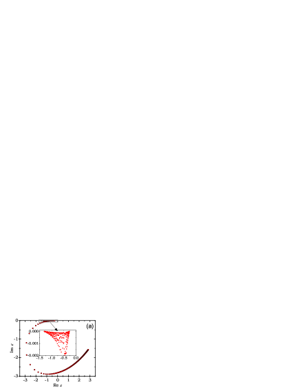
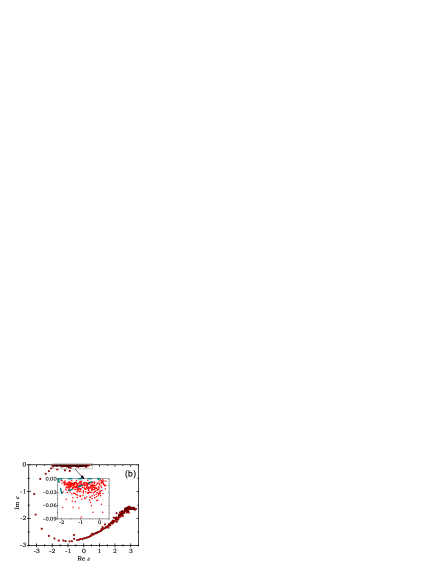
Figure 1: Complex valued spectrum of the TEM interaction matrix (9) with $k=1$ for (a) homogeneous ($W=0$) and disordered in regimes of (b) strong ($W=2$) and (c) weak ($W=20$) coupling. The dashed square in (c) shows the region where the corresponding TEM eigenmodes are scaling critically. The eigenmodes corresponding to the eigenvalues in the dashed regions are selected for further statistical analysis.

We start by analyzing the spectrum of the homogenous chain on resonance (W=0) where all the diagonal element are given by $\mathcal{M}_{ii}=0-2\imath/3$. Typical spectra for TEM and TM excitations are shown in Figures 1(a) and 2(a) for $k=1$.

For $k<1.4$, the TEM eigenvalues are divided into almost-real and complex subsets. The almost-real ($\mathrm{Im}\,{\varepsilon}\ll\mathrm{Re}\,{\varepsilon}$) subset corresponds to subradiative (bound) eigenstates. These eigenstates have a wavelength shorter than the free space propagationweber_propagation_2004; koenderink_complex_2006 and cannot couple to the outgoing radiation, except at the two ends of the chain. The eigenmodes corresponding to complex eigenvalues ($\mathrm{Im}\,{\varepsilon}\sim\mathrm{Re}\,{\varepsilon}$) are superradiative. For these modes a constructive interference in the far-field enhances the scattering from each particle in comparison with the an isolated one.

From the form of expansion (6) it is clear the eigenstates with (close to) zero eigenvalues will dominate the response of the system to external excitation. However, different regions in the spectrum can be experimentally probed by two approaches: Firstly, by changing the lattice spacing, or secondly, by detuning from the resonance frequency, which will add a constant real number to the diagonal of the interaction matrix $\mathcal{M}$. Close to the resonance this number is linearly proportional to the frequency variation. This shift results in driving a different collective excitation, which has obtained the closest eigenvalue to the origin of the complex plane.

IV.2 The effect of disorder

As mentioned before, disorder is introduced to the system by adding random numbers from the interval $[-W/2,W/2]$ to the diagonal of $\mathcal{M}$. With this setting, the parameter space has two coordinates $W$ and $k$, and $g=(Wk)^{-1}$ is the coupling parameter. The weak and strong coupling regimes correspond to $g\ll 1$ and $g\approx\mathcal{O}(1)$ respectively. For $k<0.5$ the short range behavior is dominated by the quasi-static part of the interaction. The eigenstates of the disordered chain are thus exponentially decaying –similar to localized states. Since we are mainly interested in the critical behavior of eigenfunctions we focus on the region with $0.5<k<3$.

IV.2.1 Small disorder

In the intermediate and strong coupling regime, the spectrum of the disordered matrix keeps the overall form of the homogeneous case (where the real part of the diagonal is zero), as can be seen in Figures 1(b) and 2(b).

At the sub-radiative band-edge of the TEM spectrum, modes of different nature mix due to disorder. This region is magnified in the inset of Fig. 1(b). The eigenmodes corresponding to this region are of hybrid character. They consist of separate localization centers that are coupled via extended tails of considerable weight. The typical size of each localized section is longer than the interparticle spacing. Similar modes have been observed in a quasi-static investigation of two-dimensional planar compositesstockman_localization_2001. For one-dimensional systems they are sometimes called necklace states in the literature pendry_quasi-extended_1987; bertolotti_optical_2005. Heuristically, this behavior can be attributed to the disorder induced mixing of sub-radiative and super-radiative modes which have closeby eigenvalues in the complex plain. Further evidence for this mixed behavior will be later discussed based on the shape of PDF in section IV.3.2.

For TM polarization all of the eigenstates become exponentially localized with power-law decaying tails. The localization length increases towards the band center. Therefore, in a chain with finite length, one will see two crossovers in the first Brilluoin zone, from localized to extended and back. However, the nature of localization seems to be different at the two ends. The subradiative modes ($\mathrm{Im}\,{\varepsilon}\ll\mathrm{Re}\,{\varepsilon}$) are localizaed due to interference effects similar to the Anderson localization while the superradiative modes ($\mathrm{Im}\,{\varepsilon}\sim\mathrm{Re}\,{\varepsilon}$) are localized by radiation losses. These two crossover regions eventually approach each other and disappear as the amount of disorder is increased, leading to a fully localized spectrum of eigenmodes. The spectral behavior is more complicated for higher wavenumbers with $k>\pi$ but a discussion on that is further than the scope of this article.

IV.2.2 Large disorder

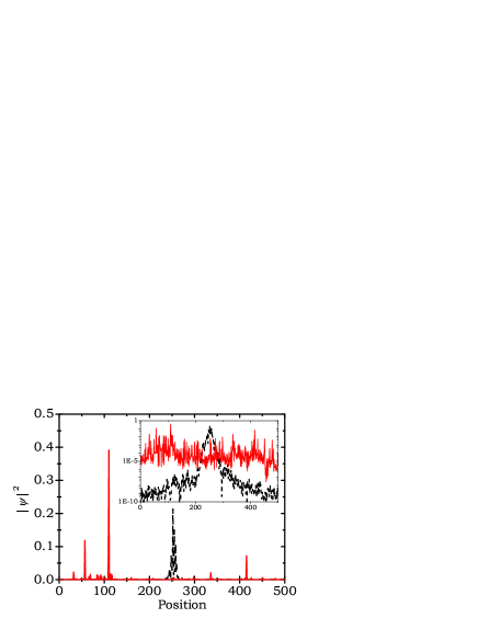
Figure 3: Typical TEM critical (red solid line) and TM localized (black dashed line) eigenvectors of matrices defined in section II.3 with $k=1$ and $W=10$. The inset shows the same plot in logarithmic scale.

In the weak coupling regime, the matrix is almost diagonal and thus the eigenvalues just follow the distribution of the diagonal elements. Typical eigenstates are shown in Fig. 3. As will be shown later, for this regime, all the eigenstates for TEM and TM are localized (since the coupling is weak) except for a band (about 20% width) of TEM eigenstates with the most negative real part of their eigenvalues. The states in this band show multifractal (critically extended) behavior for any arbitrarily weak coupling. Existence of these states is one of the major results of this investigation and their statistical analysis is the main subject of interest in the rest of this report.

The multifractality of eigenfunction in the weak coupling regime is inline with the prediction of the virial expansion result (17). However our theory cannot describe why only a part of the TEM eigenstates are critically extended and the rest of them are localized, according to the numerical results.

IV.3 Scaling behavior of PDF

The scaling of PDF is an effective tool for analyzing the localized to extended transition in sample with finite length rodriguez_multifractal_2009; rodriguez_critical_2010; schubert_distribution_2010. We also use this statistical indicator to distinguish the regions of critical scaling. Only those eigenmodes for which their scaled PDF for different system sizes overlap are critical. For the wavefunctions that fulfill this criteria, the scaling of GIPR is analyzed. This second analysis confirms the presence of critical behavior by checking the the power-law scaling behavior. The logarithmic slope gives the multifractal dimensions. We have preformed extensive survey of the size-scaling behavior of PDF over the $W,k$ space with $~{}10^{4}$ eigenfunctions for each configuration.

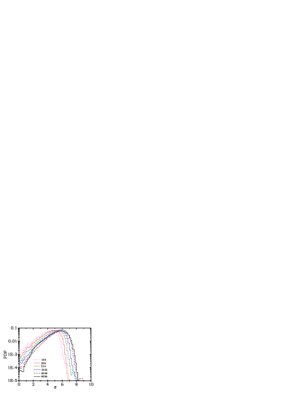
Figure 4: Scaling of PDF for TM eigenmodes for different lengths of the chain and correspondingly scaled box sizes of $b=2^{-6}\times L$. Different line types (and colors) correspond to different system sizes as indicated by the legend. $W=30$ and $k=1$. The shift of the peak to the larger values of $\tilde{\alpha}$ indicates that the eigenmodes are localized.

For each system size the scaled PDF is approximated by a histogram $\mathcal{P}(\ln I_{B}/\ln(b/L))$ over the sampled eigenfunctions These histograms are shown in Figures 4 to 7 for different models. The shift of the peak of the distribution toward larger values (higher density of darker points) by an increase in the system size is a signature of eigenmode localization. A shift in the opposite direction towards a Guassian distribution with a peak at $\tilde{\alpha}_{m}=d=1$ is characteristic of the extended states. Overlap of these histograms signifies the critical behavior of the eigenmodes.

IV.3.1 TM and TEM modes in the weak coupling regime

The typical scaling of PDF for TM modes is shown in Fig. 4. It clearly reveals the localized behavior of these eigenfunctions. This is the generic behavior observed for these modes at any point in the parameter space. This result is in agreement with the Levitov’s prediction, since the coupling is decaying as $r^{-2}$. Localization in disordered one dimensional systems has already been studied extensively and we do not discuss it further in this article.

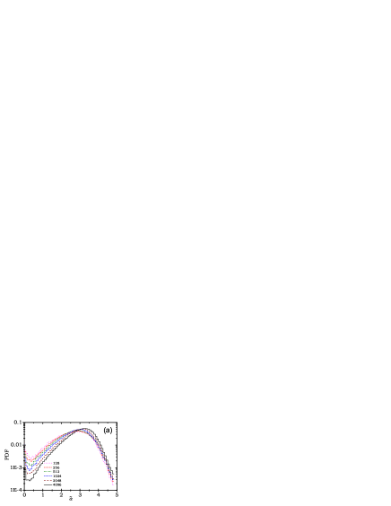
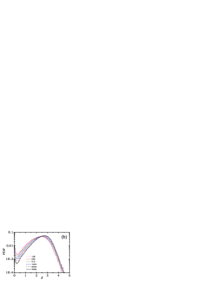
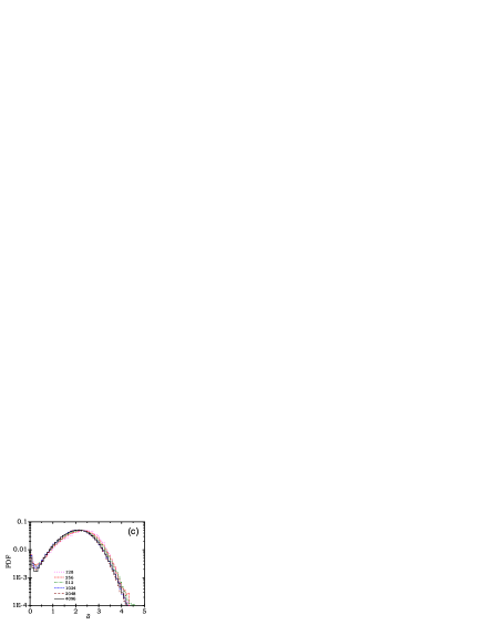
Figure 5: Same as Fig. 4 for TEM eigenmodes. For each figure 12% of the eigenmodes are used with (a) most positive, (b) closest to zero, and (c) most negative real part of their eigenvalues. Critical scaling is only observed in (c). The shift in the peak of the distribution shows that the rest of the eigenmodes are localized.

In the regime of weak coupling, $Wk>10$, the numerical results show convincing indication of critical scaling in a band of the TEM modes. These results are plotted in Fig. 5. The band of critical modes consists of those with the most negative real part of their eigenvalues. Outside this band the eigenfunctions show scaling behavior similar to localized modes as shown in Fig. 5(a) and (b). This crossover from localized to critical eigenfunctions may be useful for measuring the critical exponent. However, critical exponent must be defined based on a proper ordering of eigenvalues, which is known to be a non-trivial task for complex eigenvalues.

IV.3.2 TEM modes in the strong coupling regime

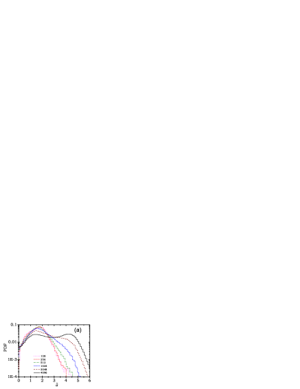
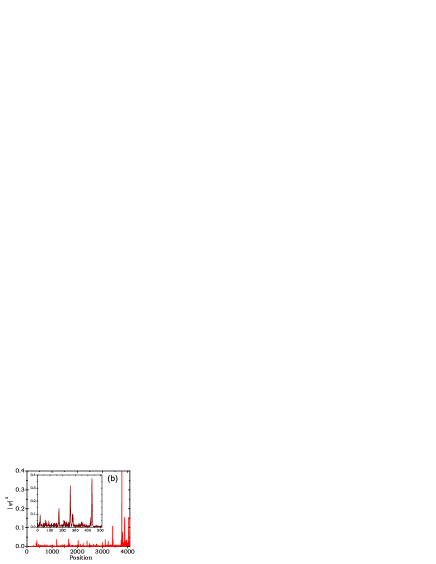
Figure 6: (a) Similar to Fig. 4 for TEM modes in the regime of strong coupling with $k=1$ and $W=0.7$. The analyzed eigenmodes are selected from the spectral region indicated by the dashed triangle in Fig. 1(b). (b) Typical eigenmodes used for the PDF in (a) for two system lengths $L=4096$ and $L=512$ (inset).

In the strong coupling regime, i.e. weak disorder, we have found it more representative to order the complex eigenvalues by their argument. A narrow region near the negative real axis is selected as shown in Fig. 1(b). The histograms representing the scaled PDF of these eigenfunctions are plotted in Fig. 6(a). These histograms do not overlap so the criticality cannot be verified. Meanwhile, the behavior is neither representative of the localized modes nor the extended modes. It appears that the overall extent of the state is comparable with the system size even for the longest chain, but it has an strongly fluctuating internal structure, similar to critical states. Typical eigenmodes of this regime are shown in Fig. 6(b). Since the scaled PDF histograms do not overlap, we cannot prove the multifractal nature of the states with a formal logarithmic scaling. Describing the true nature of these modes and their statistical behavior needs further theoretical modeling.

IV.3.3 PDF of the intermediate models

The results of the perturbation calculations in Sec. III.1 are insensitive to the details of the model. Therefore they cannot describe some of our observations that are based on direct numerical diagonalization. For example, according to the perturbation theory, all the TEM modes in the weak coupling regime must be critical. This prediction does not agree with the simulation results since PDF scaling in observed for only part of these modes. The same numerical analysis on Hermitian random banded matrices perfectly matches the results of perturbation results.

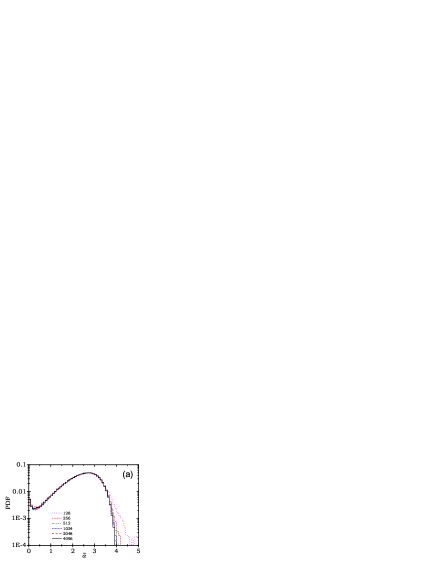
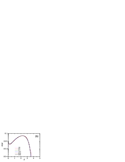
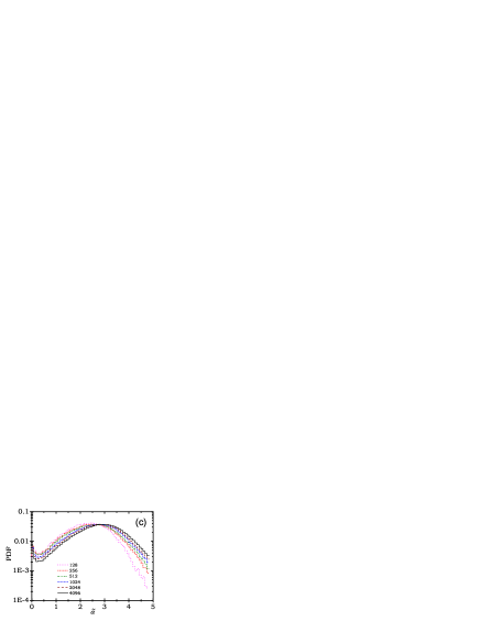
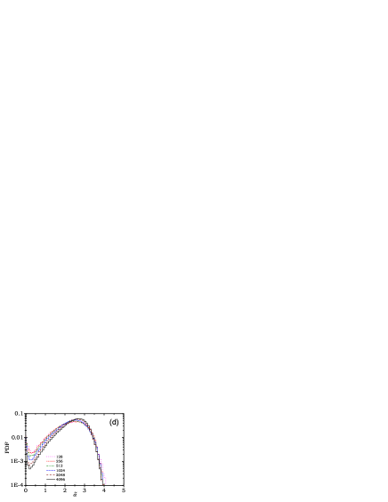
Figure 7: Similar to Fig. 4 for models (a) H0, (b) H1, (c) H2, and (d) C1. Critical scaling is observed for H0 and H1 models. The eigenvectors of the H2 and C1 models are localized. These models are defined in Sec. II.4.

To further explore the origin of this deviation for complex-symmetric matrices of our model for TEM excitations, we have performed the same numerical procedures on the hypothetic models introduced in Sec. II.4. The PDF scaling graphs for these models are depicted in Fig. 7. All these results are for the regime of weak coupling with the same $W$ and $k$.

1. The matrices in this model are orthogonal and they are the closest to the frequently used PLRBM ensemble with an interaction decay exponent $\mu=1$. The PDF shows perfect scaling as depicted in Fig. 7(a). The statistics is obtained by sampling from 12% of the eigenvectors at the band center, with eigenvalues closest to zero. The analysis shows the same critical behavior (not shown) for the two ends of the spectrum. These results also confirm that our choice of numerical precision and sampling is sufficient for the essential conclusions we get.

2. These matrices are also Hermitian like model H0. The magnitude of the off-diagonal elements is not random, but follows the decay profile of TEM complex-valued coupling (9). Only the phase is randomized. Critical scaling of the eigenfunctions is again evident from the PDF scaling depicted in Fig. 7(b).

3. This ensemble of complex-symmetric matrices resembles the TEM model. The phases of the off-diagonal elements are randomized like the model H1. The finite-size scaling of PDF, depicted in Fig. 7(c) shows the behavior that is attributed to localized modes. For localized eigenvectors the peak of the distribution shifts toward higher values of $\alpha$, which signifies a higher density for points with a low intensity.

4. This model is the Hermitian form of TEM coupling matrix. The difference between this model and H1 is in the phase factor, which is kept periodic like the original Green function. The only random elements of these matrices are the diagonal ones. Despite the minor difference between models H1 and H2, the result of PDF scaling analysis is completely different. These results are depicted in Fig. 7(d) and show that the eigenvectors are localized. This observation is inconsistent with the perturbation theory, which predicts critical behavior for this model like H0 and H1. It is important to point out that the considered periodicity for the interaction phase $k=1$ is incommensurate with the periodicity of the lattice, which equals $2\pi$ in our redefinition of units.

IV.4 Multifractal analysis

Since the critical scaling of part of the TEM eigenmodes in the weak coupling regime is clearly observed in the scaling of PDF, we apply generic techniques of multifractal(MF) analysis to quantify the MF spectrum and compare it with our theoretical results.

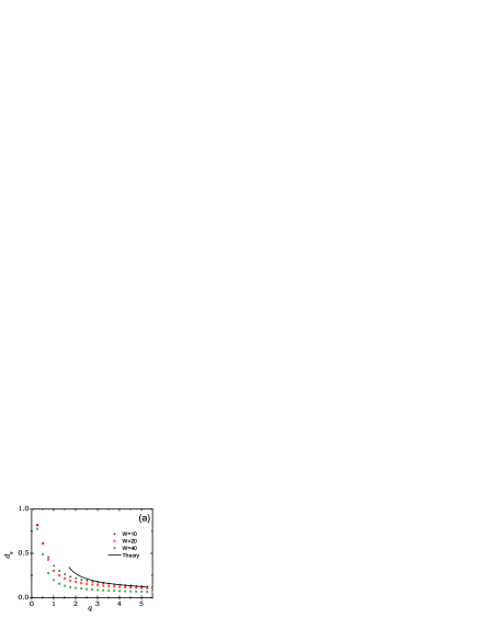
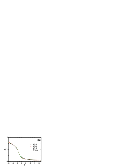
Figure 8: The anomalous dimensions $d_{q}$ (symbols) at a fixed coupling strength for (a) TEM critical modes and (b) Hermitian matrices H1 are compared with the corresponding results (solid line) (17) and (18) from perturbation analysis. For Hermitian matrices, the symmetry relation predicted in Ref. [mirlin_exact_2006] is used for plotting the theoretical curve at negative $q$. The errors estimated from the least squares fitting routine are smaller than the symbol sizes and are not shown. The largest error in $d_{q}$ for point $q=5.5$ on the graph is $\pm 0.02$.

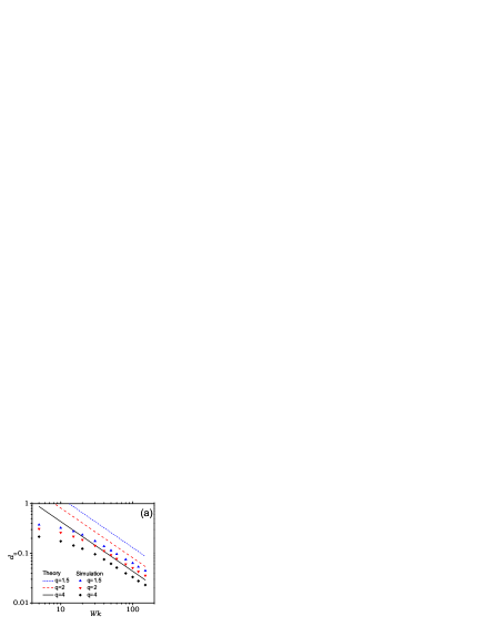
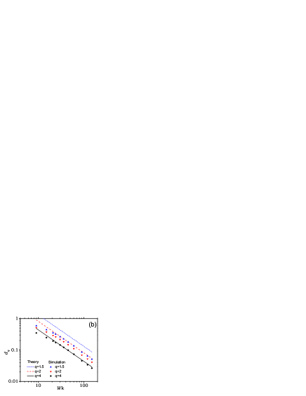
Figure 9: The anomalous dimensions $d_{q}$ extracted from direct numerical diagonalization (symbols) for three different values of $q$ are compared with the perturbation results (lines) of Eq. (17) in the weak coupling regime for different values of disorder and (a) $k=1$ or (b) $k=3$. The numerical results converge to the theory slowly.

We have used both size scaling and box scaling methods for extracting the scaling exponents of GIPR for several different parameters. We do not observe significant differences in the results of either method (comparison not shown). Therefore, due to its faster computation, we use the box scaling analysis on the largest system sizes, $L=4096$, to extract the anomalous exponents $d_{q}$ for several values of $W$ and $k$. A summary of these results for different values of disorder strength is depicted in Figures 8 and 9. To show the precision of the numerical analysis, we have also performed this analysis for Hermitian model H1. The results are shown in Fig. 8(b) and compared with the theoretical prediction of Eq. (18). Excellent matching between theory and simulation is evident for the Hermitian case. However, for the complex-symmetric matrices (corresponding to TEM coupling) the numerical results show significant deviations from the prediction of perturbation analysis, indicating that the first order virial expansion is insufficient for describing that model.

In particular, according to Eq.(17) $d_{q}$ is proportional to the coupling strength $g\equiv(Wk)^{-1}$ in the weak coupling regime. The results of direct diagonalization show, in contrast, a dependence of $d_{q}$ on $W$ at a fixed value of $g$. This fact can be seen in Fig. 8(a). The numerical results are systematically lower than the theoretical prediction for $k<3$.

Furthermore, the dependence of MF dimensions on the coupling strength is checked for $9\leq Wk\leq 150$. The results are shown in Fig. 9 for $k=1$ and $k=3$. The overall inverse linear behavior is observed for $Wk>30$. But the quantitative correspondence between the numerical results and prediction (17) from perturbation analysis is only met for the large values of $k$ and high moments of GIPR, $q>3$.

IV.5 The singularity spectrum

Another frequently used representation of the multifractality is called the singularity spectrum, $f(\alpha)$. This representation is completely analogous to the one using anomalous dimensions. For the sake of completeness, we also show this representation for two of the models that are critical in their scaling behavior.

The singularity spectrum $f(\alpha)$ is the fractal dimension of the subset of those points in the wavefunction for which intensity scales as $L^{-\alpha}$. It is related to the set of anomalous exponents $\tau(q)\equiv d_{q}(q-1)$ by a Legendre transform

$$f(\alpha)=q\alpha-\tau(q),\;\;\;\;\alpha=\tau^{\prime}(q)\;\;\;q=f^{\prime}(\alpha),.$$ (19)

The quantity $\alpha$ introduced here is related by an irrelevant scaling prefactor to $\tilde{\alpha}$, which was used for the definition of PDF. However, specially for a skewed PDF, this prefactor can significantly deviate from unity and therefore $\alpha$ and $\tilde{\alpha}$ are not exactly equivalent quantities.

For a precise derivation of $\alpha$ and $f(\alpha)$ one has to perform a full scaling analysis on the intensity distribution. This is either possible by applying relation (19) to the calculated set of anomalous exponents or by a direct processing of the wavefunction intensities. The latter method, which was introduced by Chhabra and Jensen chhabra_direct_1989, is computationally superior. For this method there is no need for a Legendre transform, which is very sensitive to the numerical uncertainties.

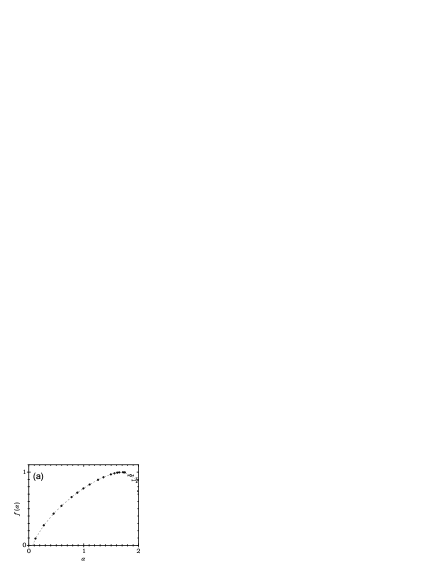
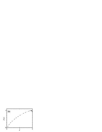
Figure 10: The multifractal spectrum $f(\alpha)$ for (a) TEM critical modes and (b) Hermitian matrices H0 extracted directly from the eigenvectors by using the method of Chhabra and Jensen chhabra_direct_1989. For both graphs $W=30$ and $k=1$. The error bars indicate to the standard deviation among 20 realizations of disorder and are smaller than the symbol size for most of the data points. The dashed lines are guides to the eye.

We have applied the direct determination method to extract the singularity spectrum for TEM critical eigenfunctions and the Hermitian model H0. The results are shown in Fig. 10. As can be seen in both graphs, the position of the peak of the spectrum is different from the peak of the corresponding PDF plots, $\tilde{\alpha}_{m}$, which are presented in Figures 5(c) and 7(a). This difference is due to the large skewness of the PDF resulted from the very weak coupling regimes that are considered in this article.

For the Hermitian critical models the domain of $\alpha$ is restricted to $(0,2d)$ due to the symmetry relationmirlin_exact_2006 of $f(\alpha)$. Yet, there is no proof that this symmetry also holds for non-Hermitian matrices. From our data, it seems plausible that this symmetry is actually broken and there are some points with $\alpha>2$. However, to provide a strong numerical evidence for this statement one has to analyze much larger ensembles with higher numerical precision, which is beyond the scope of the current article.

V Summary and Conclusion

We have investigated, theoretically and numerically, the statistical properties of the eigenmodes of a class of complex-symmetric random matrices, which describe the electromagnetic propagation of polarization waves in a chain of resonant scatterers. We have found that all of the TM modes are localized in the weak coupling regime. The TEM modes in this regime show critical behavior due to the $r^{-1}$ dependence in the dyadic Green function. This critical behavior is in agreement with the results of the method of virial expansion for almost diagonal matrices. We have used this method to calculate the MF spectrum of TEM modes.

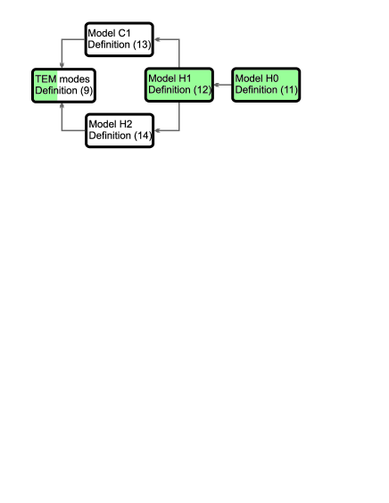
Figure 11: Summary of the scaling analysis on PDF of eigenvectors of matrices from various models. The intermediate hypothetic models transform the Hermitian RBM to the model describing TEM coupling. The colored boxes indicate those models that show critical scaling behavior. The model indicated by white boxes have localized eigenvectors. For TEM modes, only a part of the spectrum is critical.

Although the perturbation theory suggests criticality for all TEM modes, the numerical analysis shows this type of scaling only for part of the spectrum in the complex plain. This is understandable in the sense that the first oder result of the perturbative approach gives an oversimplified picture, which is insensitive to details of the model such as a non-trivial phase dependence of the matrix elements. To reveal which aspect of the TEM coupling accounts for the existence of a critical band in the spectrum, we have analyzed three intermediate models. These models have properties between the dipole chain interaction matrix and power-law Hermitian banded random matrices. The summary of the scaling results for all these models is shown in Fig. 11. It seems that both non-Hermitian character of the TEM coupling and the periodic phase of the interaction between dipoles is important for the observed critical eigenmodes.

Our analysis also resulted in another unexpected finding. The eigenvectors of Hermitian banded matrices with $r^{-1}$ coupling are no longer critically scaling if the interaction phase is set periodically. In our model H2, the randomness is only on the diagonal. Based on the PDF scaling results, we clearly see that the eigenvectors are localized. This is in contrast with the commonly believed conjecture that an interaction potential with a phase that is incommensurate with the lattice can be considered as random.

Criticality of wavefunctions has been studied theoretically and numerically for several models in the context of condensed matter physics. Recently, such wavefunctions have been observed near the Anderson transition for elastic wavesfaez_observation_2009 and electronic density of states at an interfacerichardella_visualizing_2010. The recent advances in optical and microwave instrumentation makes it possible to experiment in details the propagation of electromagnetic waves in artificially made structures. Our report points out to those systems in which such critical phenomena can be directly measured. These measurements provide a lot of insight for generic models of wave transport in disordered system.

VI Acknowledgements

We thank Yan Fyodorov, Femius Koenderink, and Eugene Bogomolny for fruitful discussions. This work is part of the research program of the “Stichting voor Fundamenteel Onderzoek der Materie”, which is financially supported by the “Nederlandse Organisatie voor Wetenschappelijk Onderzoek”. AO acknowledges support from the Engineering and Physical Sciences Research Council [grant number EP/G055769/1].

Appendix A Perturbation results for eigenvector moments

In the regime of the strong multifractality, i.e. when $Wk\gg 1$, the density of states is determined only by the distribution of the diagonal elements and hence is uniform. Therefore we assume that all eigenvectors are characterized by the same scaling exponents and we define the ensemble average GIPR as

$$\langle P_{q}\rangle = \frac{1}{L}\sum_{n=1}^{L}\sum_{i=1}^{L}|\psi_{n}(x_{i})|^{2q}.$$ (20)

The moments of the eigenvectors can be extracted from the powers of the diagonal elements of the Green functions and therefore can be computed using the method of the the virial expansion.

In the first order of the virial expansion, which corresponds to a pure diagonal matrix, the eigenvectors consists of only one non-zero component and therefore all moments are equal to one due to normalization: $\langle P_{q}\rangle^{(1)}=1$.

In the next order of the virial expansion the contribution to the eigenvectors moments from all possible pairs of two levels of the unperturbed system should be taken into account. Thus we need to calculate the moments of the eigenvectors of the following $2\times 2$ matrices:

$$M(i,j) = \left(\begin{matrix}E_{i}&\mathcal{M}_{ij}\\ \mathcal{M}_{ji}&E_{j}\end{matrix}\right),$$ (21)

Denoting by $P_{q}(i,j)$ the moments of the second component of the corresponding eigenvectors we have

$$\langle P_{q}\rangle^{(2)}=\frac{1}{L}\sum_{i\neq j}^{L}(P_{q}(i,j)-1)$$ (22)

The subtraction of $1$ in the equation above eliminates the contribution already taken into account in the diagonal approximation.

Let us introduce the following notation for $M(i.j)$:

$$H(i,j) = \left(\begin{matrix}E_{1}&he^{\imath\phi}\\ he^{\imath\phi}&E_{2}\end{matrix}\right),$$ (23)

where $E_{1}\equiv E_{i}$, $E_{2}\equiv E_{j}$ and $he^{\imath\phi}\equiv\mathcal{M}_{ij}=\mathcal{M}_{ji}$. Below we also denote $P_{q}(i,j)$ by $P_{q}$. As the eigenvectors of $H(i,j)$ do not depend on the absolute values of the matrix elements, but only on their relative ratios, we may assume now that $E_{1}$ and $E_{2}$ are distributed uniformly in $[-1/2,1/2]$ and $h=e^{ik|i-j|}/Wk|i-j|$. For the reasons which will be described later, the other terms in the coupling elements are not considered here. By the assumption of weak coupling $|h|\ll 1$ and writing the eigenvectors of $M(i,j)$ explicitly, we obtain:

$$P_{q} = \int_{-1/2}^{1/2}dE_{1}\int_{-1/2}^{1/2}dE_{2}(Q((E_{1}-E_{2})/h)+Q((E_{2}-E_{1})/h)),$$

$$Q(x) = \left(\frac{4}{4+\left(x-\sqrt{(x^{2}+4e^{-2i\phi}}\right)\left(x-\sqrt{(x^{2}+4e^{2\imath\phi}}\right)}\right)^{q}.$$ (24)

In the limit $h\to 0$ one can show that $Q(r)=\theta(r)$ and thus $P_{q}=1$. This result corresponds to the diagonal approximation and is cancelled by $-1$ in Eq.(22). In order to find first non-trivial contribution we need to compute a term which is linear in $h$. To this end we first differentiate Eq.(A) with respect to $h$, then change the integration variables $\{E_{1},E_{2}\}\to\{E_{1},x=(E_{1}-E_{2})/h\}$ and consider the limit $h\to 0$:

$$\lim_{h\to 0}\frac{dP_{q}}{dh} = -2\int_{-\infty}^{\infty}dx\>xQ^{\prime}(x)\equiv-F(q,\phi).$$ (25)

The expansion of $P_{q}$ then takes the form:

$$P_{q}=1-|h|F(q,\phi)+O(h^{2}).$$ (26)

Collecting the contributions from all the off-diagonal elements we obtain

$$\langle P_{q}\rangle=1-\frac{1}{Wk}\frac{1}{L}\sum_{i\neq j}\frac{F(q,k|i-j|)}{|i-j|}.$$ (27)

Expanding $F(q,\phi)$ in the Fourier series $F(q,\phi)=\sum_{p}c_{p}(q)e^{\imath p\phi}$ we find

$$\frac{1}{L}\sum_{i\neq j}\frac{F(q,k|i-j|)}{|i-j|} = \frac{1}{L}\sum_{i\neq j}\frac{c_{0}(q)}{|i-j|}+\frac{1}{L}\sum_{i\neq j}\sum_{p\neq 0}\frac{c_{p}(q)e^{\imath pk|i-j|}}{|i-j|}$$ (28)

$$= 2c_{0}(q)\ln L+O(1),$$

so that we arrive at the following result:

$$\langle P_{q}\rangle=1-\frac{2c_{0}(q)}{Wk}\ln L,\quad c_{0}(q)=\frac{1}{\pi}\int_{0}^{2\pi}d\phi\int_{-\infty}^{\infty}dx\>xQ_{x}^{\prime}(x,q,\phi),$$ (29)

where $Q$ is defined in Eq.(A) and can be written as

$$Q(x,q,\phi)=\left(\frac{4}{4+\left|x-\sqrt{x^{2}+4e^{-2i\phi}}\right|^{2}}\right)^{q}.$$ (30)

Comparing this result with the scaling of the moments by changing the system size

$$\langle P_{q}\rangle\propto L^{-d_{q}(q-1)},$$ (31)

we find the expressions for the fractal dimensions

$$d_{q}=\frac{2c_{0}(q)}{Wk(q-1)}.$$ (32)

One can check that in the case of the orthogonal matrices, i.e. when $\phi=0$, the old result can be reproduced after the change of the variable $x=(2w-1)/\sqrt{w(1-w)}$:

$$c_{0}(q) = 2\int_{-\infty}^{\infty}dx\>xQ_{x}^{\prime}(x,q,0)$$ (33)

$$= 2\int_{0}^{1}dw\>\frac{qw^{q-3/2}(2w-1)}{\sqrt{1-w}}$$

$$= 2\sqrt{\pi}\frac{\Gamma(q-1/2)}{\Gamma(q-1)}$$

$$d_{q}(\phi=0) = \frac{4\sqrt{\pi}}{Wk}\frac{\Gamma(q-1/2)}{\Gamma(q)}$$ (34)

The result for complex-symmetric matrices deviate only slightly from the one for orthogonal case. This deviation is most pronounced around $q=2.5$.

Figure 2: Same as Fig. 1 for TM polarization.