Abstract

Detailed features of solitons in holographic superfluids are discussed. Using solitons as probes, we study the behavior of holographic superfluids by varying the scaling dimension of the condensing operator, and build a comparison to the BEC-BCS comparison phenomena. Further evidence for this analogy is provided by the behavior of solitons’ length scales as well as by the superfluid critical velocity.

1 Introduction

In recent years there has been great interest in studying superfluidity in ultracold Fermi gases. In the laboratory, one cools a gas of fermionic atoms to temperatures below a few microKelvins. By subjecting the system to a controllable external magnetic field, one can tune the interactions in the fermionic gas. Famously, what one finds is a crossover phenomenon. On one side of the range the system is described by condensed loosely bound Cooper pairs of fermions; while at the other end the fermions become very strongly bound and the system is effectively characterized as a condensate of a fundamental bosonic degree of freedom. These two extremes are separated by the unitarity point, where the systems do not have a simple description in terms of either simple bosons or fermions.

At zero temperature, precisely at the unitarity point, apart from the fermion density the system has no other length scale. This feature is of interest to holographic model building in string theory, where it has been discovered that some strongly coupled scale invariant theories have a dual description in terms of gravitational theories in asymptotically anti-de Sitter spacetimes of one higher dimension.

One of the first holographic models for a superfluid was introduced in [1]. This is a relativistic $2+1$ dimensional superfluid described holographically using a gravitational theory in $3+1$ dimensions. Using classical gravity theory, one expects to reproduce a large $N$ strong coupling limit of a dual $2+1$ dimensional system, which we will often refer to as the (dual) field theory. Typically one expects the field theory to possess both bosonic and fermionic degrees of freedom, and the operator responsible for symmetry breaking could then be a composite operator including fermions (see e.g. the discussion in [2]). It was shown in [1], that for low enough temperatures, the $U(1)$ global symmetry of the field theory is broken and that this phase, in the dual gravity description, presents itself as a black hole with complex scalar hair outside its horizon.

It is important to consider to what extent the model [1] can mimic the salient features of cold atomic systems. It is obvious that it cannot be literally interpreted as a model for such systems. The cold atoms are a $d=3$ non-relativistic system, while the holographic system describes a relativistic $d=2$ large $N$ (mean field) theory. Furthermore, it would be natural to explore the possibility to find a gravity dual for a system at unitarity in view of the conformal invariance of the gravity description. We will address the question whether there is any sense in which [1] could resemble such a system?

Firstly, it is encouraging to note that many of the features of the non-relativistic condensates are expected to have relativistic analogs, since the basic intuitions about the nature of bound states are the same [3]. Secondly, the unitarity regime was also studied without introducing a dimensionful parameter, using an $\epsilon$ expansion [4, 5].

Further [4, 5] one way to interpret the $\epsilon$ expansion study of the unitarity regime is as a family of conformal field theories separating a BCS like unitarity phase (near $d=2$) from a BEC like unitarity phase (near $d=4$) with the most interesting and strongly coupled unitarity near $d=3$. There is a natural parameter controlling the physics of the holographic condensates, namely the scaling dimension of the condensing operator. Changing the scaling dimension might be interpreted as a family of conformal field theories corresponding to different kinds of superfluids on the unitary regime as in [4, 5] . Finally we would like to point out that [3] found that, at least when approaching unitarity from the BEC side, relativistic and non-relativistic systems behave similarly.

The fact that this system is strongly coupled, involves both fermion and boson degrees of freedom, and may be studied using conformal field theory methods, suggests that it may have a degree of commonality with holographic theories [7, 8, 9]. To summarize, we adopt the point of view that the unitarity regime of cold atoms provides a nice guide to study, interpret and organize many of the features of the superfluid first described in [1], and likely other related models as well.

What would then be a suitable probe to the subtle microscopic features at both sides of unitarity? It is interesting to note that solitons in a superfluid phase provide nice probes of the short distance structure even at the mean field level, [10, 11] (at least away from the strict unitarity limit, where constructing the mean field theory is problematic). The main reason for this is that across the soliton’s core the superfluid must interpolate all the way from the broken to the symmetry restored phase. The core’s structure will have features which may be used to characterize the short distance features of the theory. An interesting example of the use of solitons in understanding the microscopic constituents of a certain supersymmetric quantum field theories may be found in [12].

As will be described, solitons in the holographic system possess several similarities with solitons found in cold atomic systems. In addition we will find that the analogy with atomic systems is useful to organize certain linear response calculations in the holographic system. Conversely, the properties of holographic solitons may be of interest for the study of their real world counterparts. Holographic duals provide a rather simple effective theory for a strongly coupled system at finite temperature. In the case of superfluids, they give a toy model for the condensate and the normal component and their interactions. For example, we can study how the charge depletion at the core of the soliton varies as a function of the temperature, which would be very difficult to do using standard condensed matter techniques.

2 One holographic model of superfluidity

Ref. [1] constructed a holographic dual for a superfluid in 2+1 dimensions, provided by an Einstein-Abelian-Higgs system in 3+1 dimensional asymptotically $AdS$ space,

$$S_{AdS}=\int d^{4}x\sqrt{-g}\Big{[}\frac{1}{\kappa_{4}^{2}}\left(\mathcal{R}+\frac{6}{L^{2}}\right)-\frac{1}{q^{2}}\Big{(}|D_{\mu}\Psi|^{2}+m^{2}|\Psi|^{2}+\frac{1}{4}F_{\mu\nu}^{2}\Big{)}\Big{]}$$ (1)

By virtue of the AdS/CFT correspondence, the gauged symmetries of the gravitational (bulk) theory correspond to global symmetries of the dual field theory (which shall also be called the “boundary theory”). Thus, the Lorentz covariance of the boundary theory follows from the bulk diffeomorphism invariance and the bulk U(1) gauge symmetry gives rise to a U(1) global symmetry in the dual field theory. We shall identify the corresponding conserved charge with the particle number in the language appropriate for atomic systems.

Spontaneous breakdown of this global symmetry will then result in a charged superfluid condensate. The formation of the condensate is dual, in the bulk gravitational theory, to spontaneous gauge symmetry breaking - that is to say, to the condensation of a scalar field charged under the gauge symmetry. The entire system maybe placed at finite temperature by including a black hole background, in which case the Hawking temperature corresponds to the equilibrium temperature of the superfluid.

Basic properties of superfluids, such as transport properties at linearized level [13, 14, 15, 16, 17] have been studied using the action (1); the derivation of non-linear superfluid dynamics has been discussed in [18].

The AdS-CFT dictionary tells us that the gravitational action in $4$ dimensions evaluated on the solutions to the equations of motion (with suitable boundary conditions) is the generating functional of various moments of the corresponding operators in the $2+1$ dimensional quantum field theory

$$e^{-S_{AdS}(onshell)}=\langle e^{-\int d^{3}x(\rho(x)\mu(x)+\mathcal{O}(x)J(x))}\rangle_{QFT}\ .$$ (2)

The metric of the bulk spacetime is required to asymptote to Anti de Sitter space (the asymptotic behaviour in fact defines the energy momentum tensor of the field theory). The boundary QFT operators are related to the behavior of the bulk fields in the asymptotically AdS regime by the relations

$$\Psi(x,z)=z^{\Delta}\langle\mathcal{O}_{\Delta}(x)\rangle+z^{3-\Delta}J(x)+...\quad A_{t}(x,z)=\mu(x)+z\rho(x)+...$$ (3)

where the mass of the bulk field $\Psi$ is

$$m^{2}=\Delta(\Delta-3).$$ (4)

In the dual field theory one identifies $J$ with the source for the operator $\mathcal{O}_{\Delta}$ of scaling dimension $\Delta$ in the dual field theory. The value $\langle\mathcal{O}_{\Delta}(x)\rangle$ occurring in (3) is identified with the expectation value of the dual operator given an external source, $J(x)$. Also $\mu(x)$ is interpreted as a chemical potential in the dual field theory, while $\rho(x)$ is the (canonically) conjugate variable, the charge(/particle number) density.

To have a well defined solution one must impose boundary conditions which fix the value of $J(x)$ in the gravitational theory. The value of $\mathcal{O}_{\Delta}(x)$ is then determined uniquely. In the remainder we will choose our units so that the AdS scale is fixed to $L=1$. For large $m^{2}$ one only finds a solution if $\Delta$ is chosen to be the largest root of (4). However, for

$$-\frac{9}{4}<m^{2}<-\frac{5}{4}\ ,$$ (5)

one obtains a sensible solution using either root of (4) (for a discussion, see e.g. [20]). In the window of two quantizations, there are two field theories with operators of different scaling dimensions, corresponding to the choice of boundary conditions.

To construct a holographic superfluid one must search for solutions to the equations of motion obtained from (1) such that the charged operator has a nonzero expectation value even after its external source is removed. Gravitationally this means that one is searching for a black hole solution with scalar hair in asymptotically AdS space. In Minkowski space such hairy black holes do not exist, but in [21] it was noted that the negative cosmological constant may stabilize hair outside a black hole.

Throughout this work we will work in the so-called probe limit, ($\frac{\kappa_{4}^{2}}{q^{2}}$ is small), so that the backreaction to gravity can be ignored. The gravitational solution involves a planar AdS-Schwarzschild metric,

$$ds^{2}=\frac{1}{z^{2}}(-f(z)dt^{2}+f(z)^{-1}dz^{2}+dr^{2}+r^{2}d\theta^{2}),$$ (6)

where $f(z)=1-z^{3}$. In the above, temperature has been absorbed in a rescaling to dimensionless coordinates. After the rescaling, the only free parameter is the dimensionless ratio $\mu/T$. Changing this ratio may be thought of as changing the temperature (chemical potential) and keeping the chemical potential (temperature) fixed. In this background, charged scalar hair may then emerge depending on the temperature.

When studying homogeneous states it is possible to go beyond the probe approximation and include back reaction from the bulk scalar and gauge fields to the black hole metric [22]. In doing so, one verifies that working with an uncharged black hole is a good approximation when the scalar field’s charge is large ($\frac{\kappa_{4}}{q}\sim.01$) and mass is small.

In order to find the dual field theory operator expectation values we need to solve the classical equations of motion in AdS space to obtain the on shell fields. In the probe approximation, the equations of motion become

$$0 =\frac{1}{\sqrt{-g}}\partial_{\mu}(\sqrt{-g}g^{\mu\nu}\partial_{\nu}R)+m^{2}R-R(\partial_{\mu}\chi-A_{\mu})^{2}$$ (7)

$$0 =\frac{1}{\sqrt{-g}}\partial_{\mu}(\sqrt{-g}F^{\mu\nu})-R^{2}(A^{\nu}-\partial^{\nu}\chi)$$ (8)

$$0 =\partial_{\mu}(\sqrt{-g}R^{2}g^{\mu\nu}(\partial_{\nu}\chi-A_{\nu})),$$ (9)

where we have defined the real valued fields $R$ and $\chi$ according to the relation $\Psi=\frac{1}{\sqrt{2}}Re^{i\chi}$.

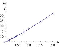
Figure 1: The critical value of the chemical potential as a function of the charged operator’s scaling dimension, while keeping the temperature fixed. $\Delta_{-}\ (\Delta_{+})$ is to the left (to the right) of 1.5 on the horizontal axis.

The scalar fields are unstable to spontaneous symmetry breaking as one raises the chemical potential $\mu$, so that above the critical value $\mu_{c}$ the boundary theory enters the superfluid phase. As we vary the mass of the bulk scalar field over the range (5), we cover the following range of scaling dimensions: $\frac{1}{2}<\Delta_{-}\leq\frac{3}{2}\ ;\ \frac{3}{2}\leq\Delta_{+}<\frac{5}{2}\ .$ Higher masses then correspond to the range $5/2\leq\Delta_{+}$.

One effect of the varying scaling dimension is a change in the critical value $\mu_{c}$ of the chemical potential where the superfluid transition happens. In Fig. 1 we have plotted $\mu_{c}$ as a function of $\Delta$. We see that operators of larger scaling dimension have larger (smaller) values of $\mu_{c}$ ($T_{c}$).

3 Solitons as a way to study the properties of the superfluid

The last section described a set of holographic superfluids which may be obtained by varying the scaling dimension and chemical potential. There are many quantities that one could study, for example the chemical potential dependence of the superfluid order parameter near the critical temperature first found in [23]

$$\langle\mathcal{O}_{\Delta}\rangle\sim\sqrt{\frac{\mu}{\mu_{c}}-1}.$$ (10)

A key question is what does one learn about the superfluids from such computations. For example, the last scaling is presumably a mean field result. For instance, one would like to know how to characterize the degrees of freedom that are the constitutents of the superfluid (since this is far from obvious in the holographic description).

There are at least three routes that one might consider. The obvious one is to come up with a detailed top-down model, with complete control over the boundary theory at the microscopic level, as in the original case of $D3$-branes and $N=4$ super-Yang-Mills theory (for work in this direction, see [2, 24, 25]). However, most models are bottom-up type, where the fundamental degrees of freedom and dynamics of the boundary theory are unknown. That leaves one two other strategies to consider.

The first is to consider linear response theory. It is straightforward to study the linear response of fields already involved in the gravity solution, but one is also interested in the way other fields, such as fermions, might respond to the superfluid. This approach is obstructed because a bottom-up approach generally lacks a stringy embedding which would dictate the allowed fermions.

The second, especially clean way to study holographic superfluids is to study kinks and vortex solutions which asymptote to the homogeneous ground states described in Section 2. The key reason is that it is known that kinks and vortices may shed light on the short distance features, even at the mean field level. Essentially this is due to the fact that the core region must interpolate all the way to the symmetric phase and hence the soliton must know about physics of all length scales. Because one expects mean field theory to still be sufficient, it is enough to look for inhomogeneous solutions to classical gravity. An advantage of spatially dependent solutions is that they are inherent to the system – one does not need to turn on any external fields to excite it.

In the rest of this Section we will discuss how to construct solitonic solutions to the gravitational equations of motion. Then we will discuss several features of the solitons found in [26, 27, 28] and an analogy with BEC-BCS, which is useful both in organizing the holographic results as well as suggesting further tests one might perform.

3.1 Method

The differential equations obtained from (1) are a set of coupled nonlinear partial differential equations which are easiest approached numerically. The basic strategy will be to exploit the fact that the equations are elliptic outside the horizon. This will allow us to construct an auxiliary heat equation which we solve numerically.

In more detail, as discussed in [28], when we work in the $A_{z}=0$ gauge and use the cylindrical symmetry the equations of motion may be brought to the following form for vortex configurations,

$$0 =f\partial_{z}^{2}\tilde{R}+(\partial_{z}f+(2\Delta_{-}-2)\frac{f}{z})\partial_{z}\tilde{R}-\Delta_{-}^{2}z\tilde{R}+\frac{1}{r}\partial_{r}(r\partial_{r}\tilde{R})$$

$$-\tilde{R}(-\frac{1}{f}A_{t}^{2}+\frac{(A_{\theta}-n)^{2}}{r^{2}})$$

$$0 =f\partial^{2}_{z}A_{t}+\frac{1}{r}\partial_{r}(r\partial_{r}A_{t})-z^{2\Delta_{-}}\tilde{R}^{2}A_{t}$$

$$0 =\partial_{z}(f\partial_{z}A_{\theta})+r\partial_{r}(\frac{1}{r}\partial_{r}A_{\theta})-z^{2\Delta_{-}}\tilde{R}^{2}(A_{\theta}-n),$$ (13)

where we have defined $\tilde{R}=z^{-\Delta_{-}}R$. A similar set of equations may be obtained for kink solutions as described in [27] for the case $m^{2}=-2$.

For both vortex and kink solutions we impose regularity conditions at the horizon. This is the same condition that was used to find the homogeneous solution, and is necessary to obtain a steady state solution. In the asymptotically AdS region we will impose a uniform chemical potential as well as a vanishing scalar non-normalizable mode. The vortex solution also involves the $\theta$ component of the gauge field, which we take to vanish at the AdS boundary. This corresponds to having no external driving vorticity to source the vortex.

The basic strategy for finding solutions is to make an initial guess at a solution (that respects the boundary conditions) and then let this guess flow according to an auxiliary heat equation. By waiting long enough in auxiliary time, we arrive at a solution of the equations of motion (13). In reality all this is done on a lattice and one stops the simulation when the evolution is suitably slow. For details of the algorithm as well as error analysis see [26]. Typical kink and vortex solutions are shown in Figs. 2 and 4.

With this method we find that we are able to obtain good numerical solutions for values of $T/T_{c}>.5$ (or $\mu/\mu_{c}<2$). See [27] for a detailed discussion of the numerics. The numerical computations were performed with MATHEMATICA and some simple C-programming using desktop computers.

3.1.1 Solutions

Kinks:

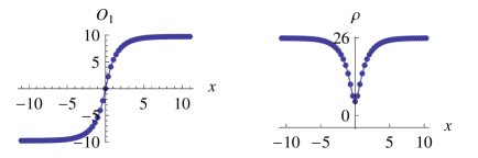
Figure 2: A typical kink soliton profile as computed using holography. On the left is the condensate’s profile plotted in the transverse coordinate. On the right is the density profile in the same transverse direction. These curves were obtained using a $\Delta=1$ condensate.

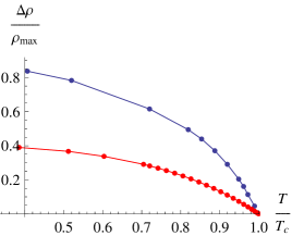
Figure 3: The core charge depletion fraction for kink solitons at $m^{2}=-2$ for varying $T/T_{c}$. $\Delta=1$ is indicated by the blue curve (top) and $\Delta=2$ is indicated by the red curve (bottom).

In Fig. 2 we have plotted a typical kink solution. We see that the condensate passes through zero, as required by topology and continuity. We also see that the (number) density does not completely vanish in the core of the soliton. A nice feature of the holographic model is that it gives an effective theory for the condensate and thermal fluctuations, so one can easily study the effects of varying temperature. In order to disentangle the thermal fluctuations, we reproduce Fig. 3 from [27] displaying the charge density’s core depletion as a function of the temperature. This graph indicates that the two superfluids have very different behavior as one lowers the temperature. Specifically, one finds that the $\Delta=2$ superfluid has an excess of charge density lying in its solitons’ cores in addition to the condensate’s contribution. This latter feature is totally different from what one would obtain from a simple Gross-Pitaevskii picture for a purely bosonic condensate at zero temperature, where the density goes to zero at the core.

Vortices:

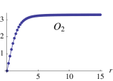
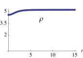
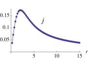
Figure 4: A typical vortex soliton profile as computed using holography. On the left is the condensate’s radial profile. In the middle is the profile of the charge density. On the right is the current density’s radial profile. These curves were obtained using a $\Delta=2$ condensate.

In Fig. 4 we have shown a typical vortex profile. Again, we find that the condensate vanishes in the vortex’s core as is expected. We also find that the charge density does not typically vanish in the core. Finally, as discussed in [28] we may identify the superfluid current from the angular component of the bulk gauge field. The superfluid current rises from zero at infinity until the critical velocity is surpassed and then falls to zero because the core is in the normal phase.

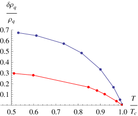
Figure 5: The core charge depletion fraction for vortex solitons at $m^{2}=-2$ for varying $T/T_{c}$. $\Delta=1$ is indicated by the blue curve (top) and $\Delta=2$ is indicated by the red curve (bottom).

As for the kink solutions, we can again easily study the effect of varying temperature. We have reproduced Fig. 5 from [28] showing the temperature dependence of the core charge depletion fraction. This figure also clearly shows that the $\Delta=2$ fluid has an ”excess” charge density in its core as compared to to the $\Delta=1$-fluid In the next Section we will remind the reader of what happens in the BEC-BCS crossover. This will serve as a useful guide to help interpret the core features of holographic solitons.

3.2 BEC-BCS analogy

In the last Section we saw that, when $m^{2}=-2$, solitons have very different core features when one changes the scaling dimension of the condensing operator. In this Section we wish to use the BEC-BCS crossover as a benchmark system to help us organize our holographic results. This will help us both to interpret the features of the holographic solitons as well as suggest further questions.

For the non-relativistic BEC-BCS crossover at zero temperature, [10, 11] have studied the behavior of kink and vortex solitons. In both papers, it was found that soliton cores in fermionic superfluids have non-vanishing number densities of cold atoms, even though the condensates vanish. This is very different than BEC solitons, where the atomic number density vanishes (at zero temperature) when the condensate vanishes. In these systems soliton cores are able to reveal the microscopic structure to the superfluid, even at the mean field level. For fermionic superfluids, as one approaches the cores, there are additional states available in the form of fermion excitations because the core is in the normal phase. On the other hand, bosonic superfluid solitons have vanishing core atomic number densities because there are no additional non-condensate states available at zero temperature. In those works, it was also found that the core structures smoothly interpolated between the BEC and BCS limits. At finite temperature, even in the BEC superfluid, we expect there will be a small contribution to the number density from the thermal cloud (non-condensate normal fluid component) which can show up in the soliton’s core.

In both [10, 11], it was argued that the solitonic cores also were able to reveal the character of the additional states carried by a fermionic superfluid’s core. Specifically, in [10], it was found that the solitons display Friedel oscillations in their cores. In [11] it was found that the oscillations in vortices were finite size effects, not Friedel oscillations. On the other hand, [11] found that the vortex cores knew about $k_{f}$ in the fact that the vortices had different length scales in the cores and tails.

Comparing the holographic superfluids to the crossover systems suggests that we should interpret excess core charge density in a soliton as a signal that there are additional non-condensate states residing in the core. Therefore, we might expect to see that one can interpolate between ”empty” and ”full” cores as one changes the gravitational mass parameter hence changing the scaling dimension [4, 5] . In addition, we may also look and see if holographic solitons identify the fermionic/bosonic character of the ”excess” states in the soliton’s core. To do this there are at least two ways to proceed. First one may try to identify whether vortices display single or multiple length scales in their cores and tails. Second, one could hope to identify any Friedel oscillations.

3.3 Varying the Scaling Dimension

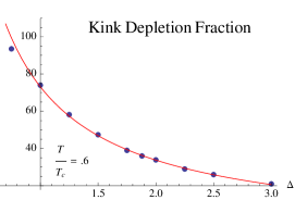
Figure 6: The charge density depletion fraction ($\times 100$) for kink solitons as a function of the condensate’s scaling dimension at $T/T_{c}=.6$. The curve is a best fit obtained for scaling dimensions above the B.F. bound ($\Delta=3/2$).

In Subsection 3.2 it was pointed out that comparing to the crossover indicates that one should expect that the charge density depletion fraction in a soliton’s core to interpolate between $0$ and $100\%$ as one varies the scaling dimension of the condensing operator (at zero temperature). In principle, it is simple to repeat the analysis in Subsection 3.1 when $m^{2}=-2$ now allowing for more general scaling dimensions. In practice, one cannot work at $0$ temperature for two reasons. First, we have assumed a probe approximation which is only valid for temperatures moderately below to $T_{c}$ ($\mu$ above $\mu_{c}$). Secondly, even if we went beyond the probe approximation, it is computationally too expensive to obtain solutions for arbitrarily low temperatures.

In order to proceed we note that in Fig. 3 and Fig. 5 the depletion fraction seems to be saturating near $T/T_{c}\sim.5$ independent of the scaling dimension. Therefore, as an approximation to the depletion fraction at low temperature we will study solitons at $T/T_{c}=.6$ as we vary $\Delta$. Finally, for the sake of brevity we will focus on the kink solitons. It is a straightforward exercise to show that vortices also display the same features as one varies $\Delta$.

In Fig. 6 we see the smoothly varying charge density depletion fraction in the core of a kink soliton at fixed $T/T_{c}=.6$. A numerical fit of the form

$$\frac{\delta\rho}{\rho_{max}}=A+\frac{B}{\Delta}$$ (14)

was made for the points with scaling dimension greater than $\Delta=3/2$. The best fit values are $(A,B)=(-.06,.8)$. The small variation in the graph is primarily due to the small uncertainty in the value of $T/T_{c}$. We note that there is a visible change in the behavior of the depletion fraction as one lowers $\Delta$, presumably saturating close to $100\%$ at $\Delta\sim 1/2$, although these values are beyond what we can currently simulate.

4 Characterizing the core states

4.1 Multiple length scales

Having seen that one can indeed control a soliton’s core charge depletion fraction by varying the condensing operator’s scaling dimension, and hence, the number of states available in the soliton’s core, we would also like to see to what extent one may try to characterize these states. The simplest way one might do this is to obtain characteristic length scales for the condensate’s profile in the core and in the asymptotic tails. In [11] it was found that bosonic superfluids essentially have one length scale, while fermionic superfluids lead to distinct length scales in the two regimes.

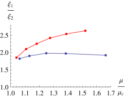
Figure 7: Here we have reproduced the graph from [28] plotting the ratio of length scales of variation as determined from the condensates profile for vortex solutions. The blue curve (bottom) indicates a $\Delta=1$ condensate and the red curve (top) indicates a $\Delta=2$ condensate.

We may try to identify how dissimilar the soliton’s length scales are according to how their ratio varies as a function of $\mu$ for different operator scaling dimensions. Fig. 7 was obtained in [28], indicating that there are two distinct length scales as one increases the scaling dimension. It would be very interesting to see what happens to the corresponding graph for $\Delta\sim 1/2$, the lowest allowed value. The comparison with the crossover would predict that in this regime the corresponding curve would be completely flat. Unfortunately, we do not have resources to say more about this value of $\Delta$. In Subsection 4 we will discuss critical velocities obtained from linear response theory. Comparing these critical velocities to the superfluid’s sound modes will lead to a morally similar comparison to Fig. 7.

4.2 Friedel Oscillations

A final feature of solitons in the crossover was the possible observation of Friedel oscillations. As discussed in [27, 28], we find no evidence of Friedel oscillations in the holographic solitons. One possible reason for the absence of the oscillations, if they exist, is that they may simply be obscured by a too large temperature.

4.3 Critical velocity

Another way to probe the constituents of a superfluid is to study superfluid flows. As one increases the velocity of the flow, it becomes energetically more favorable for the superfluid to radiate quasiparticles and go to the normal phase. The velocity at which this happens is called the critical superfluid velocity. It is possible to estimate the critical velocity using a simple kinematical argument due to Landau. According to Landau’s criterion, the critical superfluid velocity is given by the formula

$$v_{c}=\min_{k}\frac{\epsilon(k)}{k},$$ (15)

where $\epsilon(k)$ is the quasiparticle dispersion relation in the superfluid and the minimum is taken over all the quasiparticles. Strictly speaking the Landau criterion only gives an upper bound for the critical velocity and indeed at finite temperature one expects to see a smaller critical velocity than the Landau criterion tells us [29]. Still the Landau criterion can act as a useful guide in estimating the critical velocities.

For a BCS superfluid, the critical velocity is set by the lightest fermionic excitations which leads to an estimate

$$v_{c}^{BCS}\approx\frac{\omega_{gap}}{k_{f}},$$ (16)

where $k_{f}$ is the Fermi momentum and $\omega_{gap}$ is the energy gap for fermions in the superfluid phase. On the other hand on a BEC superfluid the critical velocity is set by the sound modes with lowest sound velocity $v_{s}$ so that

$$v_{c}^{BEC}\approx v_{s}.$$ (17)

Unfortunately in the holographic superfluid model we do not have a direct access to possible fermions in the system, without adding extra fields to the bulk. Even though one can access some fermionic features of the system by adding probe fermions to the bulk, the connection of these fermions to the ones possibly comprising the condensate is not very clear. Thus, we are unable to calculate the fermion dispersion relations required to get the ”fermionic” Landau criterion.

Instead we can calculate sound velocities and compare them to the critical velocity obtained from the vortex solutions. A study of the Landau criterion in the BEC-BCS crossover can be found in [30].

According to [15] the second sound has the lowest sound velocity, at least in the part of parameter space studied there. As shown in [13] the second sound can be calculated from thermodynamic quantities as

$$v_{2}^{2}=-\frac{\Big{(}\frac{\partial^{2}P}{\partial\xi^{2}}\Big{)}_{\mu,T}}{\Big{(}\frac{\partial^{2}P}{\partial\mu^{2}}\Big{)}_{\xi,T}}.$$ (18)

Here $\xi=\nabla\chi$, where $\chi$ is the phase of the condensate and the thermodynamic derivatives are evaluated at $\xi=0$. More details on the calculation may be found in [13].

The critical superfluid velocity may be obtained from the vortices as is described in [28]. One simply looks for the radial position $\rho_{*}$ inside the vortex where the condensate vanishes and evaluates the superfluid velocity at that radius. This leads to

$$v_{c}=\frac{1}{\mu}\frac{n}{\rho_{*}}.$$ (19)

A convenient way to determine $\rho_{*}$ is to identify it with the position of peak current [11, 28].

The ratio of the vortex critical velocity to the sound velocity is plotted in Fig. 8 for $T/T_{c}\approx 0.7$.

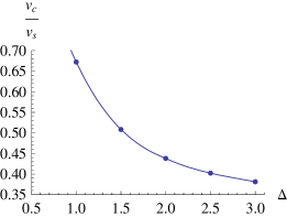
Figure 8: The ratio of the critical superfluid velocity and the second sound velocity as a function of the condensate scaling dimension. The curve in the figure is an interpolating function while the dots are the real data points.

We find that the ratio of the two velocities seems to be approaching 1 as the scaling dimension of the condensing operator is lowered, and is notably smaller than 1 as the dimension is larger. In a BEC like superfluid one would expect a sound mode to determine the critical velocity. Recalling that in our crossover analog the small scaling dimensions correspond to the supposed BEC region, we indeed find a consistent picture with the analog. In a BCS like superfluid one expects the critical velocity to be set by a fermionic excitation rather than a sound mode. Indeed it seems that in the supposed BCS region the critical velocity is likely set by something else than a sound mode.

5 Discussion

The possibility to apply holographic techniques to low dimensional systems is an exciting recent development in string theory. However, because the set of quantities which are readily computable are typically quite different, it can be difficult to develop necessary model building intuitions. For this purpose it is often useful to compare holographic constructions to known real world systems which display many features expected of holographic systems. In this article we have focused on using the BEC-BCS crossover as a guide to features observed in holographically constructed superfluids. This is a crossover from a system of fundamental bosons to fundamental fermions, both of which may display superfluidity. Most relevant for holography, this is a system which is strongly interacting and may be studied by moving along a family of fixed points [6].

We began by constructing kink and vortex solitons in holographic superfluids obtained by condensing operators of scaling dimensions $\Delta=1$ and $2$. Surprisingly their cores display different features, with the $\Delta=2$ soliton cores supporting much larger charge densities.

Similar features occur in the BEC-BCS crossover, where there are additional non-condensate states available away from BEC regime. In this setting the additional states are comprised of pre-formed bosons and fermions. Also, the solitons ”know” about the fermions in the BCS regime because the Fermi momenta controls the core size as well as any Friedel oscillations.

Comparing with the crossover physics suggested that as we vary the condensing operator’s scaling dimension we should expect the core features to smoothly interpolate as we move along the family of CFT’s. Indeed, this is precisely what was obtained. As we increased the scaling dimension, the amount of charge supported by soliton cores monotonically increased. Also consistent with this trend is the fact that the difference between core and tail length scales of variation increases with $\Delta$ [28]. Finally, from the solitons we find no signature of Friedel oscillations for $T/T_{c}>.5$.

In an effort to get a handle on the character of the excess charged states available in soliton cores we also compared the critical velocity obtained from vortex cores to the Landau critical velocity. As one lowers $\Delta$ the vortex critical velocity approaches the Landau critical velocity monotonically. This is what one would expect for a BEC superfluid.

The BEC-BCS analogy may also be used to explain results found in [23] for conductivities calculated on the superfluid phase. There it was found that there are delta function like spikes on the frequency dependent conductivity. These spikes were interpreted as due to bound states. The only bound states that may contribute to the conductivity (current-current correlator) are those that have a vanishing net charge. Thus, a natural candidate for the spikes on the BEC-BCS picture is a bound state of a fermion-hole pair. Such pairs should exist on the BCS side only. Indeed it was found in [23] that the spikes appear on the ”large” scaling dimension side, and the binding energy calculated from the position of the spikes seems to increase as the scaling dimension is lowered. This is consistent with the crossover picture where the interactions increase as one approaches unitarity from the BCS side. Holographically, as one moves across the B.F. bound ($\Delta=3/2$) to lower scaling dimensions, at some point the spikes disappear, which would seem to signal that the bound state disappears. This fits well with the BEC-BCS analogy since on the BEC side (the low scaling dimensions) the Fermi surface and light fermionic excitations are expected to completely vanish. The crossover analogy would naturally explain why the particle-hole bound state would go away.

We have shown that the BEC-BCS may be a useful guide to holographic superfluids, owing to their common strong coupling and conformal features. They also share common structures in their solitons. However to make the crossover more than an interpretational guide it would be more convincing if there was a direct signature of fermionic features in holographic superfluids. There are at least two places one might hope to find such features, first if one could cool solitons to low enough temperatures it might be possible to observe Friedel oscillations. This would be an unambiguous signal. A second route would be to try to have a better understanding of fermion probe calculations, with the hope that they could reveal any fermionic feature encoded in the bulk geometry.

6 Acknowledgements

V.K. and E.K-V. have been supported in part by the Academy of Finland grant number 1127482. E.K-V. and S.N. thank the Galilei Institute for Theoretical Physics for their hospitality and the INFN for partial support during the completion of this work. V.K. thanks the Nordic Institute of Theoretical Physics (NORDITA) for their hospitality and support while finishing this article. K.P.Y. thanks the Helsinki Institute of Physics for hospitality while this work was in progress.

References

- [1] S. A. Hartnoll, C. P. Herzog and G. T. Horowitz, Phys. Rev. Lett. 101, 031601 (2008) [arXiv:0803.3295 [hep-th]].
- [2] S. S. Gubser, C. P. Herzog, S. S. Pufu et al., Phys. Rev. Lett. 103, 141601 (2009). [arXiv:0907.3510 [hep-th]].
- [3] Y. Nishida and H. Abuki, Phys. Rev. D 72 (2005) 096004 [arXiv:hep-ph/0504083].
- [4] Y. Nishida and D. T. Son, Phys. Rev. Lett. 97 (2006) 050403 [arXiv:cond-mat/0604500].
- [5] Y. Nishida and D. T. Son, Phys. Rev. A 75 (2006) 063617 [arXiv:cond-mat/0607835].
- [6] P. Nikolic and S. Sachdev, Phys. Rev. A 75, 033608 (2007) [arXiv:cond-mat/0609106].
- [7] Y. Nishida and D. T. Son, Phys. Rev. D 76 (2007) 086004 [arXiv:0706.3746 [hep-th]].
- [8] D. T. Son, Phys. Rev. D 78, 046003 (2008) [arXiv:0804.3972 [hep-th]].
- [9] K. Balasubramanian and J. McGreevy, Phys. Rev. Lett. 101, 061601 (2008) [arXiv:0804.4053 [hep-th]].
- [10] M. Antezza, F. Dalfovo, L. P. Pitaevskii, and S. Stringari, Phys. Rev. A 76, 043610 (2007) [arXiv:0706.0601].
- [11] R. Sensarma, M. Randeria, and T. L. Ho, Phys. Rev. Lett. 96 (2006) 090403 [arXiv:cond-mat/0510761].
- [12] B. Collie, D. Tong, JHEP 0908 (2009) 006. [arXiv:0905.2267 [hep-th]].
- [13] C. P. Herzog, P. K. Kovtun, D. T. Son, Phys. Rev. D79 (2009) 066002. [arXiv:0809.4870 [hep-th]].
- [14] P. Basu, A. Mukherjee, H. -H. Shieh, Phys. Rev. D79 (2009) 045010. [arXiv:0809.4494 [hep-th]].
- [15] C. P. Herzog, A. Yarom, Phys. Rev. D80 (2009) 106002. [arXiv:0906.4810 [hep-th]].
- [16] A. Yarom, JHEP 0907 (2009) 070. [arXiv:0903.1353 [hep-th]].
- [17] I. Amado, M. Kaminski, K. Landsteiner, JHEP 0905 (2009) 021. [arXiv:0903.2209 [hep-th]].
- [18] J. Sonner, B. Withers, Phys. Rev. D82 (2010) 026001. [arXiv:1004.2707 [hep-th]].
- [19] P. Breitenlohner, D. Z. Freedman, Annals Phys. 144 (1982) 249.
- [20] V. Balasubramanian, P. Kraus, A. E. Lawrence, Phys. Rev. D59, 046003 (1999). [hep-th/9805171].
- [21] S. S. Gubser, Phys. Rev. D 78, 065034 (2008) [arXiv:0801.2977 [hep-th]].
- [22] G. T. Horowitz, M. M. Roberts, JHEP 0911, 015 (2009). [arXiv:0908.3677 [hep-th]].
- [23] G. T. Horowitz, M. M. Roberts, Phys. Rev. D78 (2008) 126008. [arXiv:0810.1077 [hep-th]].
- [24] J. P. Gauntlett, J. Sonner and T. Wiseman, Phys. Rev. Lett. 103 (2009) 151601 [arXiv:0907.3796 [hep-th]].
- [25] J. P. Gauntlett, J. Sonner and T. Wiseman, JHEP 1002 (2010) 060 [arXiv:0912.0512 [hep-th]].
- [26] V. Keranen, E. Keski-Vakkuri, S. Nowling and K. P. Yogendran, Phys. Rev. D 80 (2009) 121901 [arXiv:0906.5217 [hep-th]].
- [27] V. Keranen, E. Keski-Vakkuri, S. Nowling and K. P. Yogendran, Phys. Rev. D 81 (2010) 126011 [arXiv:0911.1866 [hep-th]].
- [28] V. Keranen, E. Keski-Vakkuri, S. Nowling et al., Phys. Rev. D81 (2010) 126012. [arXiv:0912.4280 [hep-th]].
- [29] P. Navez, R. Graham, Phys. Rev. A 73, 043612 (2006).
- [30] R. B. Diener, R. Sensarma, M. Randeria, Phys. Rev. A 77 (2008) 023626. [arXiv:0709.2653v2 [cond-mat]].