Vortex flow for a holographic superconductor

Abstract

We investigate energy dissipation associated with the motion of the scalar condensate in a holographic superconductor model constructed from the charged scalar field coupled to the Maxwell field. Upon application of constant magnetic and electric fields, we analytically construct the vortex flow solution, and find the vortex flow resistance near the second-order phase transition where the scalar condensate begins. The characteristic feature of the non-equilibrium state agrees with the one predicted by the time-dependent Ginzburg-Landau (TDGL) theory. We evaluate the kinetic coefficient in the TDGL equation along the line of the second-order phase transition. At zero magnetic field, the other coefficients in the TDGL equation are also evaluated just below the critical temperature.

I Introduction

Much attention has been given to the application of the AdS/CFT (anti-de Sitter/conformal field theory) duality Maldacena:1997re to condensed matter physics after discovery of holographic superconductor models Gubser:2008px ; Hartnoll:2008vx . Since the AdS/CFT duality is a valuable tool for investigating strongly coupled gauge theories, the application might offer new insight into the investigation of strongly interacting condensed matter systems where perturbative methods are no longer available.

The holographic superconductor model constructed by charged scalar condensate Hartnoll:2008vx is classified into type II superconductors, as it possesses vortex solutions Albash:2009ix ; Albash:2009iq ; Montull:2009fe ; Maeda:2009vf in a background magnetic field. Furthermore, it has been shown that a triangular vortex lattice solution is the most favorable solution thermodynamically just below the second order phase transition at long wavelengths Maeda:2009vf . As already seen in Refs. Maeda:2008ir ; Hartnoll:2008kx ; Maeda:2009wv , these equilibrium states are described by the Ginzburg-Landau (GL) theory. This suggests that non-equilibrium states of the holographic superconductor in the background magnetic field are also described by the time dependent Ginzburg-Landau (TDGL) theory. Indeed, it has been observed that the dynamics in the absence of magnetic field is described by the TDGL theory Maeda:2009wv ; AmadoKaminskiLandsteiner2009 ; mkf2009 .

Motivated by this, we investigate the non-equilibrium steady state of the vortex lattice solution Maeda:2009vf in the presence of a small constant electric field $E$. According to the TDGL theory, the vortex flows at a constant velocity in a direction perpendicular to both the magnetic and electric fields so that the Lorentz force on the vortex is balanced by the background electric force. The energy dissipation associated with the vortex motion occurs in the core of the vortex (vortex flow resistance), as the superconducting state disappears there.

In the TDGL equation, the evaluation of the kinetic coefficient $\Gamma$ (for example, see Eq.(B)) is important in observing the dissipation process or the spectrum of quasi-particles around the core of the vortex. While it is generically difficult to derive the coefficient from the microscopic point of view in strongly interacting condensed matter systems, it can be evaluated in the holographic model. So, it is interesting to explore the dissipation mechanism associated with the vortex motion in the framework of the AdS/CFT duality.

In this article, we perturbatively construct the vortex flow solution as a series expansion of the small electric field $E$ and derive the R-current just below the critical temperature where the scalar condensate begins. We find that vortices flow at a constant velocity and that the Ohmic dissipation occurs associated with the vortex motion, as predicted by the TDGL theory. The kinetic coefficient $\Gamma$ is evaluated along the line of the second order phase transition in comparison with the TDGL theory. In the absence of magnetic field, we also derive the other coefficients in the TDGL equation from the value of the the scalar condensate, the correlation length, and the London equation Maeda:2008ir .

The plan of our paper is as follows: In Sec. II, we expand equation of motion for the scalar field as a series in $E$. In Sec. III, we perturbatively construct the vortex flow solution by Green function method. In Sec. IV, we derive the net R-current by solving Maxwell equation and evaluate the kinetic coefficient. We briefly review the TDGL theory in Appendix B, and the other coefficients in the TDGL equation are derived in Appendix C. Conclusions and discussion are devoted to Sec. V.

II Basic equations in Eddington-Finkelstein form

We consider the (2+1)-dimensional holographic superconductor model described by a dual gravitational theory in four dimensions ($\text{AdS}_{4}$) coupled to a charged complex scalar field $\Psi$ and a Maxwell field $A_{\mu}$ Gubser:2008px ; Hartnoll:2008vx . For simplicity, we take a probe limit where the backreaction of the matter field onto the geometry can be ignored Hartnoll:2008vx .

The background metric is given by $\text{AdS}_{4}$-Schwarzschild black hole with metric

$$ds^{2}=\frac{L^{2}\alpha^{2}}{u^{2}}(-h(u)dt^{2}+dx^{2}+dy^{2})+\frac{L^{2}du^{2}}{u^{2}h(u)},$$ (1a)

$$h(u)=1-u^{3},\hskip 28.45274pt\alpha(T)=4\pi T/3~{},$$ (1b)

where $L$ and $T$ are the AdS radius and the Hawking temperature, respectively. We take the coordinate $u$ such that the AdS boundary is located at $u=0$ and the horizon is set to be $u=1$.

Under the probe limit, the action of the matter system $S=(L^{2}/2\kappa_{4}^{2}e^{2})\hat{S}$ is written by

$$\hat{S}=\int d^{4}x~{}\sqrt{-g}\left(-\frac{F^{2}}{4}-|D\Psi|^{2}-m^{2}|\Psi|^{2}\right),$$ (2)

where $m$ and $e$ are the mass and charge of the scalar field $\Psi$, respectively, and

$$D_{\mu}:=\nabla_{\mu}-iA_{\mu}~{}, F_{\mu\nu}:=\partial_{\mu}A_{\nu}-\partial_{\nu}A_{\mu}~{}.$$ (3)

Hereafter, we consider the action (2) in the simple case $m^{2}L^{2}=-2$. The equations of motion are given by

$$D^{2}\Psi+\frac{2}{L^{2}}\Psi=0~{},$$ (4a)

$$\nabla_{\nu}F_{\mu}{}^{\nu}=j_{\mu}:=i[(D_{\mu}\Psi)^{\dagger}\Psi-\Psi^{\dagger}(D_{\mu}\Psi)]~{}.$$ (4b)

For a gauge choice, we choose a gauge $A_{u}=0$ in the metric (1). The asymptotic behavior of $\Psi$ and $A_{\mu}~{}(\mu=t,x,y)$ near the AdS boundary are

$$\Psi \simeq c_{1}(t,x,y)\,u+c_{2}(t,x,y)\,u^{2}~{},$$ (5a)

$$A_{\mu} \simeq\mathcal{A}_{\mu}(t,x,y)+\mathcal{J}_{\mu}(t,x,y)\,u~{}.$$ (5b)

According to the AdS/CFT dictionary, the expectation values of the dual scalar operator ${\cal O}_{2}$ with conformal dimension two and the R-current $J^{\mu}~{}(\mu=t,x,y)$ are represented by the coefficient $c_{2}$ and $\mathcal{J}_{\mu}$ as

$$\left\langle~{}\mathcal{O}_{2}~{}\right\rangle=\left.\frac{\sqrt{2}\,e}{L\,\alpha}\,\frac{\delta S}{\delta c_{1}^{\dagger}}\,\right|_{u=0}=\frac{\sqrt{2}\,L^{3}\,\alpha^{2}}{2\,\kappa_{4}^{2}\,e}\,c_{2}~{},$$ (6a)

$$\left\langle~{}J^{\mu}~{}\right\rangle=\left.\frac{\delta S}{\delta\mathcal{A}_{\mu}}\,\right|_{u=0}=\frac{L^{2}\,\alpha}{2\,\kappa_{4}^{2}\,e^{2}}\,\eta^{\mu\nu}\,\mathcal{J}_{\nu}~{},$$ (6b)

respectively. We consider the condensation of the scalar operator ${\cal O}_{2}$, and impose an asymptotic boundary condition $c_{1}=0$ to eliminate the source term in the dual theory.

Since we are interested in the superconducting region just below the second order phase transition, the amplitude of the scalar field $|\Psi|$ is very small. So, one can expand $\Psi$ and $A_{\mu}$ in powers of a small parameter $\epsilon$ as

$$\Psi=\epsilon^{1/2}\,\psi+O(\epsilon^{3/2})~{}, A_{\mu}=\bm{\bm{A}}_{\mu}+\epsilon\,a_{\mu}+O(\epsilon^{2})~{}.$$

Then, Eq. (4b) at $O(\epsilon^{0})$ is reduced to

$$\nabla_{\nu}\bm{\bm{F}}_{\mu}{}^{\nu}=0,$$ (7)

where $\bm{\bm{F}}_{\mu\nu}=\partial_{\mu}\bm{\bm{A}}_{\nu}-\partial_{\nu}\bm{\bm{A}}_{\mu}$. By Eqs. (4), the equations of motion for $\psi$ and $a_{\mu}$ become

$$\bm{\bm{D}}^{2}\psi+\frac{2}{L^{2}}\psi=0~{},$$ (8a)

$$\nabla_{\nu}f_{\mu}{}^{\nu}=i\,\left[~{}(\bm{\bm{D}}_{\mu}\psi)^{\dagger}\psi-\psi^{\dagger}(\bm{\bm{D}}_{\mu}\psi)~{}\right]~{},$$ (8b)

where $\bm{\bm{D}}_{\mu}$ and $f_{\mu\nu}$ are defined by $\bm{\bm{D}}_{\mu}:=\partial_{\mu}-i\,\bm{\bm{A}}_{\mu}$ and $f_{\mu\nu}:=2\,\partial_{[\mu}a_{\nu]}$, respectively.

We consider a zeroth order solution of Eq. (7) generating a constant electric field $E$ and the (upper) critical magnetic field $B_{c2}$ at the second order phase transition Maeda:2009vf . This is given by the following form:

$$\bm{\bm{A}}_{t}=\mu(1-u)~{}, \bm{\bm{A}}_{x}=-E\,(t-u_{*})-B_{c2}\,y~{},$$ (9)

where $u_{*}:=\int^{u}du/\alpha h(u)$ and $\mu$ is the chemical potential. The boundary conditions at the horizon $u=1$ are determined by the regularity condition, i.e., $\bm{\bm{A}}_{t}(x,y,u=1)=0$ and $|\bm{\bm{F}}^{2}(x,y,u=1)|<\infty$. Our strategy is to solve Eqs. (8) perturbatively for small $E$ under the external gauge field (9). In the $E=0$ case, Eq. (8a) is solved as the Landau problem Albash:2008iv , and Eq. (8b) is also formally solved Maeda:2009vf .

Let us expand Eqs. (8) in powers of $E$ as

$$\psi=\psi_{0}+E\,\psi_{1}+\cdots~{},$$ (10a)

$$a_{\mu}=a^{(0)}_{\mu}+E\,a^{(1)}_{\mu}+\cdots~{}.$$ (10b)

As shown later, it is convenient to adopt an advanced null coordinate $v:=t-u_{*}$ and a coordinate $\hat{y}$ defined by

$$\hat{y}:=y+\frac{E}{B_{c2}}\,v~{}.$$ (11)

Under the coordinate transformation $(t,u,x,y)\mapsto(v,u,x,\hat{y})$, the metric (1) and the gauge field (9) are transformed as

$$ds^{2}=\frac{L^{2}\alpha^{2}}{u^{2}}\bigg{(}-h(u)\,dv^{2}-\frac{2}{\alpha}\,dv\,du+dx^{2}+d\hat{y}^{2}$$

$$\hskip 56.9055pt-\frac{2E}{B_{c2}}\,d\hat{y}\,dv\bigg{)}+O(E^{2})~{},$$ (12a)

$$\bm{\bm{A}}_{v}=\mu(1-u),\quad\bm{\bm{A}}_{u}=\frac{\bm{\bm{A}}_{v}}{\alpha\,h(u)},\quad\bm{\bm{A}}_{x}=-B_{c2}\,\hat{y}.$$ (12b)

Thus, the external electric field $E$ appears only via the metric in the Eddington-Finkelstein form (12a).

If the holographic superconductor obeys conventional type II superconductors, the vortex flows at a constant velocity $-E/B_{c2}$ along the $y$-direction by the Lorentz force. This implies that there is a “static” vortex solution in the metric (12a). So, we take an ansatz for the scalar field $\psi$:

$$\psi(x,\hat{y},u)=\int^{\infty}_{-\infty}\frac{dp}{\sqrt{2\pi}}~{}C(p)\,e^{ipx}\,\xi(\hat{y},u;p),$$

$$\xi(\hat{y},u;p)=\xi_{0}(\hat{y},u;p)+E\,\xi_{1}(\hat{y},u;p)+\cdots~{}.$$ (13a)

Defining the differential operators $\mathfrak{L}_{p}$ and $\mathcal{L}$ as

$$\mathfrak{L}_{p}:=\mathcal{L}+\frac{1}{\alpha^{2}}\left[\frac{\partial^{2}}{\partial\hat{y}^{2}}-(p+B_{c2}\,\hat{y})^{2}\right],$$ (14a)

$$\mathcal{L}:=u^{2}\frac{\partial}{\partial u}\frac{h(u)}{u^{2}}\frac{\partial}{\partial u}+\frac{\mu^{2}(1-u)^{2}}{\alpha^{2}\,h(u)}+\frac{2}{u^{2}}~{},$$ (14b)

we obtain the equations of motion for $\xi_{0}$ and $\xi_{1}$ from Eq. (8a) as

$$\mathfrak{L}_{p}\,\xi_{0}=0~{},\hskip 56.9055pt\mathfrak{L}_{p}\,\xi_{1}=\mathfrak{j}~{},$$ (15a)

$$\mathfrak{j}:=\frac{2}{\alpha B_{c2}}\,\frac{\partial}{\partial\hat{y}}\left(u\,\frac{\partial}{\partial u}\,\frac{1}{u}-\frac{i\mu(1-u)}{\alpha h(u)}\right)\xi_{0}~{}.$$ (15b)

The boundary conditions of $\Psi$ are represented by

$$\Psi(x,\hat{y},u)=\begin{cases}~{}c_{2}(x,\hat{y})\,u^{2}&(u\to 0)\\ ~{}\text{regular}&(u\to 1)\end{cases}~{}.$$ (16)

III The construction of the vortex flow solution

In this section, we construct the solutions $\xi_{0}$ and $\xi_{1}$ of Eqs. (15a). Following the ansatz in Ref. Maeda:2009vf , we separate the variable $\xi_{0}$ as $\xi_{0}=\rho_{n}(u)D_{n}(Y_{p})$, where $Y_{p}$ is defined by

$$Y_{p}:=\sqrt{2B_{c2}}\left(\hat{y}+\frac{p}{B_{c2}}\right).$$ (17)

The equations for $\rho_{n}(u)$ and $D_{n}(Y_{p})$ are derived from Eq. (15a) as

$$\mathcal{L}\,\rho_{n}(u)=\frac{B_{c2}\lambda_{n}}{\alpha^{2}}\,\rho_{n}(u)~{},$$ (18a)

$$\left(\frac{\partial^{2}}{\partial Y_{p}^{2}}-\frac{Y_{p}^{2}}{4}\right)D_{n}(Y_{p})=-\frac{\lambda_{n}}{2}\,D_{n}(Y_{p}),$$ (18b)

where $\lambda_{n}$ is a separation constant. The solution of the equation (18b) satisfying the boundary condition $\lim_{|Y|\to\infty}|D_{n}(Y)|<\infty$ is given by

$$\lambda_{n}=2n+1\hskip 28.45274pt(n=0,1,2,\cdots)~{},$$ (19a)

$$D_{n}(Y):=\left(\frac{1}{\sqrt{2\pi}\,2^{n}n!}\right)^{1/2}\,H_{n}\left(\frac{Y}{\sqrt{2}}\right)\,e^{-Y^{2}/4}~{},$$ (19b)

where $H_{n}$ is the Hermite function defined by

$$H_{n}(z):=(-1)^{n}e^{z^{2}}\frac{\partial^{n}}{\partial z^{n}}(e^{-z^{2}}).$$ (20)

The function $D_{n}(Y_{p})$ in Eq. (19b) is the $n$-th energy eigenfunction of a harmonic oscillator centered at $\hat{y}=-p/B_{c2}$ and it exponentially decays for large $|Y_{p}|$. As discussed in Ref. Maeda:2009vf , the upper critical value $B_{c2}$ is determined by $n=0$ and the solution $\rho_{0}$ satisfying the two boundary conditions (16) was numerically obtained. Therefore, we shall adopt $n=0$ solution, $\xi_{0}=\rho_{0}(u)\,D_{0}(Y_{p})$ as the leading order solution of Eq. (15a).

We derive the next order solution $\xi_{1}$ of Eq. (15a) by constructing Green function. In general, $\xi_{1}$ includes a component proportional to $\xi_{0}$. Hereafter, we shall remove this component from $\xi_{1}$ because it can be absorbed into the leading order solution $\xi_{0}$.

Introducing the inner product for $D_{n}$ as

$$(\xi,\,\eta):=\int_{-\infty}^{\infty}dY~{}\xi^{\dagger}(Y)\,\eta(Y)~{},$$ (21)

$\{D_{n}\}$ forms a complete orthonormal set

$$(D_{n},\,D_{m})=\delta_{nm}~{},$$ (22a)

$$\sum_{n=0}^{\infty}D_{n}(Y_{p})D_{n}^{\dagger}(Y^{\prime}_{p})=\delta(Y_{p}-Y^{\prime}_{p})=\frac{\delta(\hat{y}-\hat{y}^{\prime})}{\sqrt{2B_{c2}}}~{}.$$ (22b)

As well known, $\{D_{n}\}$ satisfies the relation

$$(D_{n},\,YD_{m}) =\begin{cases}\sqrt{n+1}&~{}~{}m=n+1\\ \sqrt{n}&~{}~{}m=n-1\\ 0&~{}~{}|m-n|\neq 1\end{cases}~{}{\color[rgb]{1,0,0}.}$$ (23)

In terms of the complete orthonormal set $\{D_{n}\}$, let us construct the Green function $G_{p}(u,\hat{y}\,|\,u^{\prime},\hat{y}^{\prime}\,)$ of the operator $\mathfrak{L}_{p}$ in the form

$$\frac{G_{p}(u,\hat{y}\,|\,u^{\prime},\hat{y}^{\prime}\,)}{\sqrt{2B_{c2}}}=\sum_{n=1}^{\infty}\,g_{n}(u,u^{\prime})\,D_{n}(Y_{p})\,D_{n}^{\dagger}(Y_{p}^{\prime})~{}.$$ (24)

Suppose that the two point function $g_{n}$ $(n=1,2,\cdots)$ is the solution of the equation

$$\left(\mathcal{L}-\frac{B_{c2}\lambda_{n}}{\alpha^{2}}\right)g_{n}(u,u^{\prime}\,)=\delta(u-u^{\prime})~{}$$ (25)

satisfying the boundary condition (16). Then, using the completeness of $D_{n}(Y)$ in Eq. (22b), we find that $G_{p}$ satisfies

$$\mathfrak{L}_{p}\,G_{p}(u,\hat{y}\,|\,u^{\prime},\hat{y}^{\prime}\,)=\delta(\hat{y}-\hat{y}^{\prime}\,)\delta(u-u^{\prime}\,)$$

$$\hskip 28.45274pt-\sqrt{2B_{c2}}\,\delta(u-u^{\prime}\,)\,D_{0}(Y_{p})\,D_{0}^{\dagger}(Y_{p}^{\prime})~{}.$$ (26)

This indicates that $G_{p}$ is the Green function in the solution space orthogonal to the component $\xi_{0}\propto D_{0}$.

In terms of the Green function $G_{p}$, the formal solution of $\xi_{1}$ is represented as

$$\xi_{1}(\hat{y},u;p)=\int du^{\prime}d\hat{y}^{\prime}~{}G_{p}(u,\hat{y}\,|\,u^{\prime},\hat{y}^{\prime}\,)\,\mathfrak{j}(\hat{y}^{\prime},u^{\prime};p)~{}.$$ (27)

Substituting Eq. (24) into the solution (27) and using the orthogonality condition (22a), one obtains

$$\xi_{1}(\hat{y},u;p)=-\frac{2}{\alpha\,\sqrt{2B_{c2}}}\,D_{1}(Y_{p})$$

$$\times\int^{1}_{0}du^{\prime}~{}g_{1}(u,u^{\prime}\,)\left(u^{\prime}\frac{d}{du^{\prime}}\,\frac{1}{u^{\prime}}-\frac{i\mu(1-u^{\prime})}{\alpha h(u^{\prime})}\right)\rho_{0}(u^{\prime})$$

$$=:-\frac{D_{1}(Y_{p})}{\alpha\,\sqrt{2B_{c2}}}\,\big{\{}\rho_{R}(u)+i\,\rho_{I}(u)\big{\}}~{},$$ (28)

where $\rho_{R}$ and $\rho_{I}$ are the real and imaginary parts of the $u^{\prime}$-integral, respectively.

IV Energy dissipation associated with the vortex flow

In this section, we investigate energy dissipation caused by the vortex flow solution constructed in the previous section. As shown below, the R-current associated with the vortex flow agrees with the one predicted by the TDGL theory (see, Appendix B). So, we can evaluate the kinetic coefficient $\Gamma$ in the TDGL equation (B) from the R-current. The other coefficients are also evaluated from our earlier results Maeda:2008ir in Appendix C. We begin by calculating the R-current induced by the vortex flow.

IV.1 R-current

$\left\langle~{}J^{x}~{}\right\rangle$ in Eq. (6b) can be expanded as a series in $\epsilon$ near the second order phase transition as

$$\left\langle~{}J^{x}~{}\right\rangle=\frac{L^{2}E}{2\kappa_{4}^{2}e^{2}}+\delta\left\langle~{}J^{x}~{}\right\rangle~{},$$ (29)

where $\delta\left\langle~{}J^{x}~{}\right\rangle=O(\epsilon)=O(\Psi^{2})$. The first term is caused by the normal fluid, which is independent of the vortex motion. Hereafter, we will calculate the subleading term $\delta\left\langle~{}J^{x}~{}\right\rangle$, as it is induced by the vortex motion.

For simplicity, we shall focus attention on calculating the net (total) current $\overline{\delta\left\langle~{}J^{x}~{}\right\rangle}$. We define the net value $\bar{A}$ of a quantity $A$ in the original coordinate $(x,y)$ as

$$\bar{A}:=\iint dxdy~{}A.$$ (30)

By Eqs. (5b) and (6b), $\overline{\delta\left\langle~{}J^{x}~{}\right\rangle}$ becomes

$$\overline{\delta\left\langle~{}J^{x}~{}\right\rangle}(t) =\frac{L^{2}\alpha\epsilon}{2\kappa_{4}^{2}{e^{2}}}\,\iint dxdy~{}\partial_{u}a_{x}\big{|}_{u=0}$$

$$=\frac{L^{2}\alpha\epsilon}{2\kappa_{4}^{2}{e^{2}}}\,\partial_{u}\bar{a}_{x}\big{|}_{u=0}~{}.$$ (31)

We first derive $\bar{a}_{x}$ by solving Eq. (8b). As in Eq. (10), the net bulk current $\bar{j}_{x}$ can be expanded as

$$\bar{j}_{x}=\bar{j}^{(0)}_{x}+E\,\bar{j}^{(1)}_{x}+\cdots~{}.$$ (32)

The leading term $\bar{j}^{(0)}_{x}$ is clearly zero because the current circulates (see, Ref. Maeda:2009vf ) as

$$j_{x}^{(0)}=-\epsilon\,\partial_{y}|\psi_{0}|^{2}.$$ (33)

This implies that the leading term $\bar{a}^{(0)}_{x}$ in Eq. (10b) is zero, and that $\bar{a}_{x}$ is written by $\bar{a}_{x}=E\,\bar{a}^{(1)}_{x}+\cdots$.

By Eqs. (22a), (23), and (III), the subleading term $\bar{j}^{(1)}_{x}$ is calculated as

$$\bar{j}^{(1)}_{x} =-2\epsilon\overline{\Im\left[(D_{x}\psi_{0})^{\dagger}\psi_{1}+(D_{x}\psi_{1})^{\dagger}\psi_{0}\right]}$$

$$=-\frac{2\epsilon\,\mathcal{C}}{\alpha\sqrt{2B_{c2}}}\,\rho_{0}(u)\,\rho_{R}(u)~{},$$ (34a)

$$\mathcal{C} :=\int dp~{}|C(p)|^{2}~{},$$ (34b)

which is independent of the coordinate $v$. In the spirit of finding the solution of Eq. (8b), we assume that $\bar{a}^{(1)}_{\mu}$ is also $v$-independent. Then, averaging the $x$-component of Eq. (8b) and using Eq. (34), we find

$$\frac{d}{du}\,\left(h\,\frac{d\bar{a}^{(1)}_{x}(u)}{du}\right) =\frac{2\,L^{2}\,\mathcal{C}}{\alpha\sqrt{2B_{c2}}u^{2}}\,\rho_{0}(u)\,\rho_{R}(u).$$ (35)

Here, we used the fact that the spatially averaged value in Eq. (30) is zero for the derivative terms of $a_{\mu}$ with respect to the spatial coordinates, $x$, $y$, i. e. , $\overline{\partial_{x}a_{\mu}}=\overline{\partial_{y}a_{\mu}}=0$. The regularity of $\bar{a}^{(1)}_{x}$ at the horizon determines the solution as

$$\frac{d}{du}\,\bar{a}_{x}^{(1)}(u)=-\frac{2\,L^{2}\,\mathcal{C}}{\alpha\sqrt{2B_{c2}}h(u)}\,\int^{1}_{u}du^{\prime}~{}\frac{\rho_{0}(u^{\prime})\,\rho_{R}(u^{\prime})}{u^{\prime 2}}~{}.$$ (36)

Substituting Eq. (36) into Eq. (IV.1), the net R-current becomes

$$\overline{\delta\left\langle~{}{J}^{x}~{}\right\rangle}=-\frac{\epsilon\,E\,L^{4}\,\mathcal{C}}{\kappa_{4}^{2}{e^{2}}\,\sqrt{2B_{c2}}}\,\langle\rho_{0},\,\rho_{R}\rangle,$$ (37)

where $\langle\rho_{0},\,\rho_{R}\rangle$ is the inner product defined by

$$\langle\phi,\,\psi\rangle:=\int^{1}_{0}du~{}\frac{\phi^{*}(u)\,\psi(u)}{u^{2}}.$$ (38)

Next, we express the net R-current in Eq. (37) in terms of the expectation value of the scalar operator $\left\langle~{}{\cal O}_{2}~{}\right\rangle$. Under the boundary condition (16), the operator $\mathcal{L}$ is clearly Hermitian for the inner product (38). So, using Eqs. (18a), (25), and (III), we obtain the following equality:

$$\langle\rho_{0},\,\mathcal{L}\,\rho_{R}\rangle=\frac{B_{c2}\lambda_{1}}{\alpha^{2}}\,\langle\rho_{0},\,\rho_{R}\rangle+2\left\langle\rho_{0},\,u\,\frac{d}{du}\,\frac{\rho_{0}}{u}\right\rangle$$

$$= \,\langle\mathcal{L}\,\rho_{0},\,\rho_{R}\rangle=\frac{B_{c2}\lambda_{0}}{\alpha^{2}}\,\langle\rho_{0},\,\rho_{R}\rangle~{}.$$ (39)

The boundary condition (16) simplifies the equality as

$$\langle\rho_{0},\,\rho_{R}\rangle=-\frac{\alpha^{2}}{2B_{c2}}\,\rho_{0}^{2}(u=1)~{}.$$ (40)

Substituting Eq. (40) into Eq. (37), $\overline{\delta\left\langle~{}J^{x}~{}\right\rangle}$ is expressed by the expectation value of the dual scalar operator $\left\langle~{}{\cal O}_{2}~{}\right\rangle$:

$$\overline{\delta\left\langle~{}J^{x}~{}\right\rangle} =\frac{\epsilon L^{4}\alpha^{2}}{2\kappa_{4}^{2}{e^{2}}}\,\frac{E}{B_{c2}}\,\frac{\mathcal{C}\,\rho_{0}^{2}(1)}{\sqrt{2B_{c2}}}=\frac{L^{4}\alpha^{2}}{2\kappa_{4}^{2}{e^{2}}}\,\frac{E}{B_{c2}}\,\left.\overline{|\Psi_{0}|^{2}}\,\right|_{u=1}$$

$$=\frac{\kappa_{4}^{2}\beta^{2}}{L^{2}\alpha^{2}}\frac{E}{B_{c2}}\,\overline{\left|\left\langle~{}{\cal O}_{2}~{}\right\rangle\right|^{2}}~{}.$$ (41)

Here, $\Psi_{0}:=\epsilon^{1/2}\,\psi_{0}$ and the coefficient $\beta$ is defined by

$$\beta^{2}:=\frac{\overline{|\Psi_{0}|^{2}}\,\Big{|}_{u=1}}{\overline{|c_{2}|^{2}}}=\frac{|\rho_{0}(u=1)|^{2}}{\lim_{u\to 0}|\rho_{0}(u)/u^{2}|^{2}}~{}.$$ (42)

Eq. (41) shows that a finite DC-current is induced by the motion of the scalar field in a parallel direction with the applied electric field $E$. Thus, the vortex flow resistance appears by the vortex motion in the holographic superconductor model. In the bulk side, the energy dissipation (Ohmic dissipation) associated with the resistance is represented by the energy absorption of the scalar field by the black hole. As shown in Eq. (88), the energy flows into the bulk from the boundary via the external electric field. It is transformed into the energy of the scalar field in the bulk. Since the scalar field falls into the black hole horizon, as it moves in the $y$-direction, the energy is absorbed into the black hole.

IV.2 The kinetic coefficient $\Gamma$

The form of the expectation value (41) agrees with the averaged value of the current in TDGL theory (67). Then, the kinetic coefficient $\Gamma$ is given by

$$\frac{\Gamma(T)}{e_{*}}=\left.\frac{L^{2}\mu^{2}}{\kappa_{4}^{2}}\,\frac{(\alpha/\mu)^{2}}{\beta^{2}}\,\right|_{T,B=B_{c2}(T)}=:\frac{L^{2}\mu^{2}}{\kappa_{4}^{2}}\,Z~{}.$$ (43)

We can easily show that $e_{*}=1$ in the following argument. As seen in Eq. (3), the gauge coupling between $A_{\mu}$ and $\Psi$ is given in the form, $(\partial_{\mu}-i\,A_{\mu})\Psi$. Under the gauge $A_{u}=0$, there is still a residual gauge transformation Maeda:2010br :

$$A_{\mu}(t,x,y,u) \to A_{\mu}(t,x,y,u)+\partial_{\mu}\Lambda(t,x,y)~{},$$ (44a)

$$\Psi(t,x,y,u) \to e^{i\Lambda(t,x,y)}\,\Psi(t,x,y,u).$$ (44b)

Then, Eq. (44) acts on the source $\mathcal{A}_{\mu}$ of the R-current and on the condensate $\left\langle~{}\mathcal{O}_{2}~{}\right\rangle$ dual to $\Psi$ as

$$\mathcal{A}_{\mu}(t,x,y) \to\mathcal{A}_{\mu}(t,x,y)+\partial_{\mu}\Lambda(t,x,y)~{},$$ (45a)

$$\left\langle~{}\mathcal{O}_{2}(t,x,y)~{}\right\rangle \to e^{i\Lambda(t,x,y)}\,\left\langle~{}\mathcal{O}_{2}(t,x,y)~{}\right\rangle~{}.$$ (45b)

This is a “background local U(1)” transformation of the dual field theory, indicating that the gauge coupling constant $e_{\ast}$ of $\left\langle~{}\mathcal{O}_{2}~{}\right\rangle$ is unity, i.e., $e_{\ast}=1$.

By solving numerically Eq. (18a) with $n=0$, we obtain $Z:=(\alpha/\mu\beta)^{2}=\kappa_{4}^{2}\,\Gamma/(L^{2}\mu^{2})$, which is a function of $\alpha/\mu\propto T/T_{c}$ only. In Fig. 1, we present $\Gamma(T)$ as a function of $T$. It increases as $T$ decreases from the critical temperature $T_{c}$ at zero magnetic field, $B_{c2}=0$. In the $B_{c2}\to 0$ limit ($T\to T_{c}$), both $\alpha/\mu$ and $Z$ approach critical values $\alpha_{c}/\mu\sim 0.25$ and $Z\sim 0.54$, respectively, which are independent of the critical temperature $T_{c}$. Thus, we finally obtain $\Gamma$ as

$$\Gamma(T_{c})\sim\left(\frac{L^{2}}{2\kappa_{4}^{2}}\right)303.2\times T_{c}^{2}~{}$$ (46)

in the $T\to T_{c}$ limit.

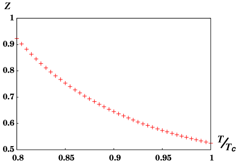
Figure 1: $T$-dependence of $Z:=\kappa_{4}^{2}\,\Gamma/(L^{2}\mu^{2})$ with $\mu$ fixed. Here $T_{c}$ is the critical temperature for $B_{c2}=0$.

V Conclusions and discussion

We have investigated the vortex motion of a holographic superconductor constructed by a gravitational model of complex scalar field coupled to the $U(1)$ gauge field. We found that the vortex flows in a direction orthogonal to both the electric field $E$ and the magnetic field $B$ at a constant velocity $v=E/B$. This is explained by the force balance between the Lorentz force and the electric force observed in the conventional type II superconductors parks .

We observed Ohmic dissipation associated with the vortex motion. This might be explained by the speculation that the superconducting state is violated at each core of the vortex lattice. In other words, the normal state at each core causes the energy dissipation by the constant motion. Since the DC-conductivity we calculated in Sec. IV is the spatially averaged value, we cannot say exactly where the dissipation occurs in the vortex motion. Indeed, the dissipation is independent of the coefficient $C(p)$ in Eq. (13). It is interesting to investigate further the location of the dissipation in our model by calculating the DC-conductivity at each point.

As shown in Sec. IV, the DC-current agrees with the current in the TDGL theory. The kinetic coefficient $\Gamma$ in the TDGL equation was obtained along the line $B=B_{c2}(T)$ in $(B,T)$ phase diagram as shown in Fig. 2. We also obtained the other coefficients in the TDGL equation just below the critical temperature $T_{c}$ at zero magnetic field. It is worth comparing these coefficients obtained in this article with the ones obtained from other phenomena as a consistency check.

In general, there is a possibility that $\Gamma$ depends on $T$ and independently on $B$, i. e., $\Gamma=\Gamma(T,\,B)$. To investigate the possibility, we need to evaluate $\Gamma$ along another line away from the $B=B_{c2}(T)$ line. It would be interesting to clarify the dependency in the phase diagram where the TDGL theory is available, and to compare it with experiments. Then, we might be able to find a sign of a strongly correlated condensed matter system in the holographic superconductor model.

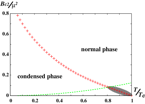
Figure 2: (color online) Phase diagram of the holographic superconductor. $B_{c2}(T)$ is marked with “$+$”(red). Since the local approximation is valid below the dashed line (green), as shown in Ref. Maeda:2009vf , the Ginzburg-Landau theory is applicable in the shaded region.

Appendix A vortex lattice solution

In the zero limit of the external electric field $E\to 0$, the solution should be reduced to the static vortex lattice solution obtained in Ref. Maeda:2009vf . Let us take $C(p)$ in Eq. (13) as

$$C(p)=\sum_{l=-\infty}^{\infty}\delta(p-p_{l})\,C_{l},$$ (47)

where $p_{l}$ and $C_{l}$ are defined by two lattice parameters, $a_{1}$ and $a_{2}$:

$$p_{l}:=\frac{2\pi\sqrt{B_{c2}}l}{a_{1}},\qquad C_{l}:=\exp\left(-i\frac{\pi a_{2}}{a_{1}^{2}}l^{2}\right).$$ (48)

In the $E\to 0$ limit, $\Psi$ has a pseudoperiodicity

$$\Psi(x,\,y,\,u)=\Psi(x+a_{1}\,r_{0},y,\,u),$$ (49a)

$$\Psi\left(x+\frac{a_{2}\,r_{0}}{a_{1}},y-\frac{2\pi r_{0}}{a_{1}},\,u\right)$$

$$\hskip 14.22636pt=\exp\left[\frac{2\pi i}{a_{1}}\left(\frac{x}{r_{0}}+\frac{a_{2}}{2a_{1}}\right)\right]\Psi(x,\,y,\,u).$$ (49b)

Thus, the fundamental region $V_{0}$ on the boundary $u=0$ is spanned by two vectors, ${\bm{b}}_{1}=a_{1}r_{0}\partial_{x}$ and ${\bm{b}}_{2}=a_{2}r_{0}/a_{1}\partial_{x}-2\pi r_{0}/a_{1}\partial_{y}$. Here $r_{0}:=1/\sqrt{B_{c2}}$ is the typical length scale of the fundamental region Maeda:2009vf . The triangular lattice solution, for example, is given by

$$\frac{a_{2}}{a_{1}}=\frac{a_{1}}{2}=3^{-1/4}\sqrt{\pi}.$$ (50)

Appendix B The vortex flow solution to TDGL equation

The conventional superconductors near the critical temperature $T=T_{c}$ are well described by the GL theory, where $T_{c}$ is the critical temperature when the applied magnetic field is zero. The free energy is represented by the order parameter ${\cal O}$ and a vector potential $\bm{\bm{A}}$ as

$$F=\int d\bm{\bm{x}}\left[c(T)|D{\cal O}|^{2}-a(T)|{\cal O}|^{2}+\frac{b(T)}{2}|{\cal O}|^{4}\right],$$

$$D:=\nabla-ie_{\ast}\bm{\bm{A}},$$ (51)

where $e_{\ast}$ is the effective charge coupled to the vector potential $\bm{\bm{A}}$. Here, we assume that the parameter $a(T)$ changes from negative to positive at $T=T_{c}$ as $T$ decreases, while the other parameters, $b$ and $c$ remain positive near $T=T_{c}$. The current $\bm{j}$ is given by

$$\bm{\bm{j}} =-\frac{\delta F}{\delta\bm{\bm{A}}}=2e_{\ast}\,c(T)\left(\Im[{\cal O}^{\dagger}\nabla{\cal O}]-e_{\ast}\,|{\cal O}|^{2}\bm{\bm{A}}\right)~{}.$$ (52)

The TDGL equation describing the non-equilibrium states is given by a kinetic coefficient $\Gamma(T)$ as

$$(\partial_{t}-ie_{\ast}\phi){\cal O}=-\Gamma(T)\,\frac{\delta F}{\delta{\cal O}^{\dagger}}$$

$$\hskip 28.45274pt=\Gamma(T)\left(c(T)D^{2}+a(T)-b(T)|{\cal O}|^{2}\right){\cal O}~{},$$ (53)

where $\phi$ is the electric potential.

We first consider the superconducting state in the absence of electric and magnetic fields. Setting the l. h. s. of (B) to zero, we obtain a stationary homogeneous solution for $T<T_{c}$ as

$${\cal O}={\cal O}_{0}(T):=\sqrt{\frac{a(T)}{b(T)}}\sim\left(1-\frac{T}{T_{c}}\right)^{1/2}=:\epsilon_{T}^{1/2}$$ (54)

near the critical temperature.

From the TDGL equation (B), the perturbation $\delta\mathcal{O}:={\cal O}-{\cal O}_{0}$ around the homogeneous condensate (54) satisfies the dispersion relation

$$\omega=-i\,c(T)\,\Gamma(T)\,\left(k^{2}+\frac{2\,a(T)}{c(T)}\right)~{},$$ (55)

where we set $\delta\mathcal{O}\propto e^{-i\omega t+i\bm{\bm{k}}\cdot\bm{\bm{x}}}$. This yields the correlation length $\xi$ from the wave number $k_{*}$ generating the static perturbation, i.e., $\omega=0$ as

$$\xi^{2}=-\frac{1}{k_{*}^{2}}=\frac{c(T)}{2a(T)}~{}.$$ (56)

Next we consider the magnetic and electric response. Applying the infinitesimal magnetic field on the homogeneous condensate (54), the London current is generated by the vector potential $\bm{A}$ as parks

$$\bm{\bm{j}}=-2\,e_{\ast}^{2}\,c(T)\,|{\cal O}_{0}|^{2}\,\bm{\bm{A}}~{}.$$ (57)

When the field strength increases beyond a critical value $B_{c1}$, the external magnetic field begins to penetrate into the superconductor and vortices appear. At $B=B_{c2}~{}(>B_{c1})$, the second order phase transition occurs and the superconductivity disappears. Just below the upper critical value $B_{c2}$, a triangular lattice appears since it is thermodynamically most favorable solution (in details, see Ref. parks ).

For simplicity, we consider the following gauge fields generating the upper critical magnetic field $B_{c2}$ and a small electric field $E$ in the $x$-direction:

$$\bm{\bm{A}}=-(B_{c2}\,y+E\,t)dx,\qquad\phi=0.$$ (58)

Substituting an ansatz

$${\cal O}(\bm{x},t)=\int dp~{}C(p)e^{ipx}\xi(\hat{y})~{}, \hat{y}:=y+\frac{E}{B_{c2}}\,t$$ (59)

into Eq. (B), we obtain

$$\frac{E}{\Gamma(T)B_{c2}}\,\frac{d\xi}{d\hat{y}} =c(T)\left[\frac{d^{2}}{d\hat{y}^{2}}-(p+e_{\ast}B_{c2}\,\hat{y})^{2}\right]\xi$$

$$+a(T)\,\xi$$ (60)

just below the critical temperature $T_{c}$. Here, we neglected the quadratic term with respect to $\xi$ because $T$ is very close to $T_{c}$ ($\epsilon_{T}$ is very small). Introducing a new variable $\chi$ as

$$\xi(\hat{y})=\exp\left(\frac{E}{2c(T)\Gamma(T)B_{c2}}\,\hat{y}\right)\chi(\hat{y})~{},$$ (61)

Eq. (B) can be simplified as

$$\left(\frac{d^{2}}{dY^{2}}-\frac{Y^{2}}{4}\right)\chi=-\frac{a(T)}{2e_{\ast}c(T)B_{c2}}\,\chi+O(E^{2})~{},$$ (62)

$$Y:=\sqrt{2e_{\ast}B_{c2}}\left(\hat{y}+\frac{p}{e_{\ast}B_{c2}}\right)~{}.$$ (63)

Neglecting the square term for small $E$ and comparing Eq. (62) with Eq. (18b), we finally obtain a vortex flow solution with the lowest energy as

$$\mathcal{O} =\int dp~{}C(p)\,\exp\left(ipx+\frac{E}{2c(T)\Gamma(T)B_{c2}}\,\hat{y}\right)$$

$$\times\exp\left[-\frac{e_{\ast}B_{c2}}{2}\left(\hat{y}+\frac{p}{e_{\ast}B_{c2}}\right)^{2}\right]$$ (64)

with the relation

$$a(T)=e_{*}c(T)B_{c2}~{}.$$ (65)

Substituting Eq. (B) into Eq. (52), we obtain

$$j_{x}=-c(T)\,e_{\ast}\,\partial_{y}|\mathcal{O}|^{2}+\frac{e_{\ast}\,E}{\Gamma(T)\,B_{c2}}\,|\mathcal{O}|^{2}~{},$$ (66a)

$$j_{y}=c(T)\,e_{\ast}\,\partial_{x}|\mathcal{O}|^{2}~{}.$$ (66b)

Averaging the values of the current over the ${\bm{x}}$-space, we find that only $\overline{j_{x}}$ is non-zero:

$$\overline{j_{x}}=\frac{e_{\ast}E}{\Gamma(T)B_{c2}}\,\overline{|{\cal O}|^{2}}~{}.$$ (67)

Eq. (67) shows the Ohmic dissipation, as the electric field is applied in the $x$-direction, i.e., ${\bm{E}}=-\partial_{t}{\bm{A}}=Edx$.

Appendix C The derivation of the coefficients in the TDGL equation

In the following, we will determine the parameters $a$, $b$, and $c$ in Eq. (B) just below the critical temperature $T_{c}$ from the correlation length and the London equation calculated in the holographic superconductor model Maeda:2008ir .

In the absence of magnetic field, the scalar field $\Psi$ and the gauge potential $A_{t}$ can be expanded as

$$\Psi(u)=\frac{\epsilon_{T}^{1/2}}{L}(\tilde{\Psi}_{1}(u)+\epsilon_{T}\tilde{\Psi}_{2}(u)+\cdots),$$

$$A_{t}(u)=\alpha(T)\{q_{c}(1-u)+\epsilon_{T}\tilde{\Phi}_{1}(u)+O(\epsilon_{T}^{2})\},$$ (68)

where $q_{c}=\mu/\alpha(T_{c})$. Then, as shown in Ref. Maeda:2008ir , the equations of motion for $\tilde{\Psi}_{1}(u)$ and $\tilde{\Phi}_{1}(u)$ are written by

$${\cal L}_{\psi}\,\tilde{\Psi}_{1}=0,\qquad\frac{d^{2}\tilde{\Phi}_{1}(u)}{du^{2}}=s(u):=\frac{2q_{c}|\tilde{\Psi}_{1}|^{2}}{u^{2}(1+u+u^{2})},$$ (69)

where ${\cal L}_{\psi}$ is defined by ${\cal L}$ in Eq. (14b) as ${\cal L}_{\psi}:=-{\cal L}|_{T=T_{c}}$. As mentioned in Sec. II, we consider the boundary conditions for $\tilde{\Psi}_{1}$:

$$\lim_{u\to 0}\tilde{\Psi}_{1}(u)=O(u^{2}),\qquad\tilde{\Psi}_{1}(u=1)=\mbox{regular}.$$ (70)

We derive the boundary conditions for $\tilde{\Phi}_{1}(u)$ from the requirement that the chemical potential $\mu=A_{t}(0)$ is fixed under the variation of the temperature:

$$\lim_{u\to 0}\tilde{\Phi}_{1}(u)=q_{c},\qquad\tilde{\Phi}_{1}(u=1)=0.$$ (71)

Here, the latter condition is the regularity condition at the horizon. The formal solution $\tilde{\Phi}_{1}$ satisfying the boundary conditions is given by

$$\tilde{\Phi}_{1}(u)=-u\int^{1}_{u}s(v)(1-v)dv$$

$$-(1-u)\int^{u}_{0}s(v)vdv+q_{c}(1-u).$$ (72)

In terms of $\tilde{\Psi}_{1}$ and $\tilde{\Phi}_{1}$, the correlation length $\xi$ is represented by

$$\xi^{2}\simeq\frac{\epsilon_{T}^{-1}}{\alpha(T_{c})}\frac{D}{N}$$ (73)

in the limit $T\to T_{c}$ , where

$$N=2\int^{1}_{0}du\left(\frac{d\tilde{\Phi}_{1}}{du}+\tilde{\Phi}_{1}(0)\right)^{2},$$

$$D=\int^{1}_{0}du\frac{\tilde{\Psi}_{1}^{2}(u)}{u^{2}}.$$ (74)

Since $\tilde{\Psi}_{1}$ is a solution of the linear equation (69), its amplitude is obtained from the next order equation:

$${\cal L}_{\psi}\tilde{\Psi}_{2}=-\frac{2q_{c}\tilde{\Phi}_{1}\tilde{\Psi}_{1}}{1+u+u^{2}}.$$ (75)

The boundary conditions for $\tilde{\Psi}_{2}$ are the same as the ones for $\tilde{\Psi}_{1}$ (70). Under the boundary conditions, ${\cal L}$ is Hermitian for the inner product (38). This yields

$$0=\langle{\cal L}_{\psi}\tilde{\Psi}_{2},\,\tilde{\Psi}_{1}\rangle=\langle\tilde{\Psi}_{2},\,{\cal L}_{\psi}\tilde{\Psi}_{1}\rangle$$

$$=-2q_{c}\left\langle\tilde{\Psi}_{1},\,\frac{\tilde{\Phi}_{1}\tilde{\Psi}_{1}}{1+u+u^{2}}\right\rangle.$$ (76)

Substituting Eq. (C) into Eq. (C), we obtain the amplitude $A$ defined by $A:=\tilde{\Psi}_{1}/\tilde{\psi}_{1}$ for a normalized solution $\tilde{\psi}_{1}$ satisfying $\tilde{\psi}_{1}(1)=1$ as

$$A^{2}=\frac{\Sigma_{2}(0)}{2\left[\int^{1}_{0}\Sigma_{1}^{2}(u)du-\left(\int^{1}_{0}\Sigma_{1}(u)du\right)^{2}\right]},$$

$$\Sigma_{n}(u)=\int^{1}_{u}\frac{(1-v)^{n}\tilde{\psi}_{1}^{2}(v)}{v^{2}h(v)}dv\qquad(n=1,\,2).$$ (77)

Numerical calculation determines the value of the amplitude $A$ and hence $c_{2}$ in Eq. (5) is evaluated as

$$c_{2}\simeq\lim_{u\to 0}\frac{\tilde{\Psi}_{1}}{u^{2}}\simeq\frac{6.55\,\epsilon_{T}^{1/2}}{L}.$$ (78)

$\xi$ in Eq. (73) is also evaluated as

$$\xi\simeq 0.0635\times\frac{\epsilon_{T}^{-1/2}}{T_{c}}.$$ (79)

For the vector potential ${\bm{A}}$ generating small magnetic field, the London equation just below $T=T_{c}$ Maeda:2008ir is evaluated as

$$\lim_{T\to T_{c}}\left\langle~{}{\bm{J}}~{}\right\rangle\simeq-\frac{L^{4}\,\alpha(T_{c})}{2\,\kappa_{4}^{2}\,e^{2}}\,\left(2\int^{1}_{0}du~{}\frac{|\Psi|^{2}}{c_{2}^{2}\,u^{2}}\right)c_{2}^{2}\,{\bm{A}}$$

$$\simeq-\frac{L^{2}\,\alpha(T_{c})}{2\,\kappa_{4}^{2}\,e^{2}}\,\left(2\int^{1}_{0}du~{}\frac{\epsilon_{T}|\tilde{\Psi}_{1}|^{2}}{c_{2}^{2}\,u^{2}}\right)c_{2}^{2}\,{\bm{A}}$$

$$\simeq-\frac{2\,\kappa_{4}^{2}}{L^{2}T_{c}^{3}}\times 1.172\times 10^{-3}\,|\left\langle~{}{\cal O}_{2}~{}\right\rangle|^{2}{\bm{A}},$$ (80)

where we used Eqs. (1b) and (6a) to derive the third equality. Comparing Eq. (C) with Eq. (57) and identifying $\left\langle~{}{\cal O}_{2}~{}\right\rangle$ with ${\cal O}_{0}$, we obtain the coefficient $c$ in the TDGL equation (B) just below $T_{c}$ as

$$c(T_{c})\simeq\frac{2\,\kappa_{4}^{2}}{L^{2}}\times\frac{5.85\times 10^{-4}}{T_{c}^{3}},$$ (81)

where we used the fact, $e_{*}=1$ derived in Sec. IV. Substitution of Eqs. (79) and (81) into Eq. (56) yields the coefficient $a$ just below $T_{c}$ as

$$a(T\to T_{c})\sim\frac{2\kappa_{4}^{2}}{L^{2}}\times\frac{0.0726\,\epsilon_{T}}{T_{c}}.$$ (82)

$b$ is also evaluated from Eqs. (6a), (54), and (78) as

$$b(T_{c})=\left(\frac{2\kappa_{4}^{2}}{L^{2}}\right)^{3}e^{2}\times\frac{2.75\times 10^{-6}}{T_{c}^{5}}.$$ (83)

Appendix D Ohmic dissipation

Since the bulk spacetime possesses Killing vector $\xi^{\mu}=(\partial_{t})^{\mu}=(\partial_{v})^{\mu}$, the energy-momentum tensor of the form

$$T_{\mu\nu} =\frac{L^{2}}{2\kappa_{4}^{2}e^{2}}\,\Bigg{[}~{}F_{\mu\lambda}F_{\nu}{}^{\lambda}+2\,\Re\left[\,\big{(}D_{\mu}\Psi\big{)}^{\dagger}\big{(}D_{\nu}\Psi\big{)}\,\right]$$

$$-g_{\mu\nu}\left(\frac{F^{2}}{4}+\big{|}\,D\Psi\,\big{|}^{2}+m^{2}\,|\Psi|^{2}\right)~{}\Bigg{]}~{},$$ (84)

satisfies the conservation law, $\nabla_{\mu}\left(T^{\mu}{}_{\nu}\,\xi^{\nu}\right)=0$. Thus, we obtain

$$0 =\int d^{4}x~{}\sqrt{-g}\,\nabla_{\mu}\left(T^{\mu}{}_{\nu}\,\xi^{\nu}\right)$$

$$=\int_{\Sigma_{f}}d\Sigma_{\mu}\,T^{\mu}{}_{\nu}\,\xi^{\nu}+\int_{\Sigma_{i}}d\Sigma_{\mu}\,T^{\mu}{}_{\nu}\,\xi^{\nu}$$

$$+\int_{\mathcal{H}}d\Sigma_{\mu}\,T^{\mu}{}_{\nu}\,\xi^{\nu}+\int_{\text{bdy}}d\Sigma_{\mu}\,T^{\mu}{}_{\nu}\,\xi^{\nu}~{},$$ (85)

where, $\Sigma_{f,i}$, $\mathcal{H}$, and bdy represent $v=\text{const.}$ null hypersurfaces, the null hypersurface at the black hole horizon, and the timelike AdS boundary, respectively. Since the spatially averaged value of $T_{\mu\nu}$ does not depend on $v$, the first and the second terms in the second line of Eq. (85) cancel each other. This implies

$$-\int_{\mathcal{H}}d\Sigma_{a}\,T^{a}{}_{b}\,\xi^{b} =\int_{\text{bdy}}d\Sigma_{a}\,T^{a}{}_{b}\,\xi^{b}~{}.$$ (86)

Due to the rapid fall-off condition for $\Psi$ (16), only the $U(1)$ bulk gauge field contributes to the boundary term in the above equation as the Ohmic dissipation:

$$\int_{\text{bdy}}d\Sigma_{a}\,T^{a}{}_{b}\,\xi^{b} =\int_{\text{bdy}}dv\,d^{2}x\left\langle~{}J^{i}~{}\right\rangle\,E_{i}~{}.$$

Here, we used the fact

$$\left\langle~{}J^{i}~{}\right\rangle=\frac{L^{2}}{2\kappa_{4}^{2}e^{2}}\,\sqrt{-g}~{}F^{ui}\,\Big{|}_{u=0},$$

$$E_{i}=-F_{ti}\,\big{|}_{u=0}=-F_{vi}\,\big{|}_{u=0} (i=x,y)~{}.$$

Hence, Eq. (86) is reduced to

$$\frac{L^{3}\,\alpha}{2\kappa_{4}^{2}e^{2}}\int_{\mathcal{H}}dv\,d^{2}x~{}\left(\delta^{ij}\,F_{vi}F_{vj}+2\,(L\,\alpha)^{2}\,\big{|}\,D_{v}\Psi\,\big{|}^{2}\right)$$

$$=\int_{\text{bdy}}dv\,d^{2}x~{}\left\langle~{}J^{i}~{}\right\rangle\,E_{i}~{}.$$ (87)

We can extract the subleading terms at $O(\epsilon)$ from above. Noting

$$\int dxdy~{}f_{vj} =\int dxdy~{}2\,\partial_{[v}a_{j]}=-\int dxdy~{}\partial_{j}a_{v}=0~{},$$

we obtain

$$\frac{L^{5}\,\alpha^{3}}{\kappa_{4}^{2}e^{2}}\int_{\mathcal{H}}dv\,d^{2}x~{}\big{|}\,\bm{\bm{D}}_{v}\Psi\,\big{|}^{2}=\int_{\text{bdy}}dv\,d^{2}x~{}\delta\left\langle~{}J^{i}~{}\right\rangle\,E_{i}~{}.$$ (88)

References

- (1) J. M. Maldacena, “The large N limit of superconformal field theories and supergravity,” Adv. Theor. Math. Phys. 2 (1998) 231 [Int. J. Theor. Phys. 38 (1999) 1113] [arXiv:hep-th/9711200].
- (2) S. S. Gubser, “Breaking an Abelian gauge symmetry near a black hole horizon,” Phys. Rev. D 78 (2008) 065034 [arXiv:0801.2977 [hep-th]].
- (3) S. A. Hartnoll, C. P. Herzog and G. T. Horowitz, “Building a Holographic Superconductor,” Phys. Rev. Lett. 101, 031601 (2008) [arXiv:0803.3295 [hep-th]].
- (4) T. Albash and C. V. Johnson, “Phases of Holographic Superconductors in an External Magnetic Field,” arXiv:0906.0519 [hep-th].
- (5) T. Albash and C. V. Johnson, “Vortex and Droplet Engineering in Holographic Superconductors,” Phys. Rev. D 80 (2009) 126009 [arXiv:0906.1795 [hep-th]].
- (6) M. Montull, A. Pomarol and P. J. Silva, “The Holographic Superconductor Vortex,” Phys. Rev. Lett. 103 (2009) 091601 [arXiv:0906.2396 [hep-th]].
- (7) K. Maeda, M. Natsuume and T. Okamura, “Vortex lattice for a holographic superconductor,” Phys. Rev. D 81, 026002 (2010) [arXiv:0910.4475 [hep-th]].
- (8) K. Maeda and T. Okamura, “Characteristic length of an AdS/CFT superconductor,” Phys. Rev. D 78, 106006 (2008) [arXiv:0809.3079 [hep-th]].
- (9) S. A. Hartnoll, C. P. Herzog and G. T. Horowitz, “Holographic Superconductors,” JHEP 0812, 015 (2008) [arXiv:0810.1563 [hep-th]].
- (10) K. Maeda, M. Natsuume and T. Okamura, “Universality class of holographic superconductors,” Phys. Rev. D 79, 126004 (2009) [arXiv:0904.1914 [hep-th]].
- (11) “Hydrodynamics of Holographic Superconductors,” Irene Amado, Matthias Kaminski, and Karl Landsteiner, JHEP 0905, 021 (2009) [arXiv:0903.2209 [hep-th]].
- (12) K. Maeda, S. Fujii, and J. Koga, “The final fate of instability of Reissner-Nordstrom-anti-de Sitter black holes by charged complex scalar fields,” Phys. Rev. D 81, 124020 (2010) [arXiv:1003.2689 [gr-qc]].
- (13) C. P. Herzog, P. K. Kovtun and D. T. Son, “Holographic model of superfluidity,” Phys. Rev. D 79, 066002 (2009) [arXiv:0809.4870 [hep-th]].
- (14) T. Albash and C. V. Johnson, “A Holographic Superconductor in an External Magnetic Field,” JHEP 0809, 121 (2008).
- (15) R. D. Parks, Superconductivity (Marcel Dekker Inc., New York, 1969); A. A. Abrikosov, Fundamentals of the Theory of Metals (North-Holland, New York, 1988); M. Tinkham, Introduction to Superconductivity (McGraw-Hill Inc., New York, 1996).
- (16) K. Maeda, M. Natsuume and T. Okamura, “On two pieces of folklore in the AdS/CFT duality,” Phys. Rev. D 82, 046002 (2010) [arXiv:1005.2431 [hep-th]].