LDPC Codes for Compressed Sensing

Abstract

We present a mathematical connection between channel coding and compressed sensing. In particular, we link, on the one hand, channel coding linear programming decoding (CC-LPD), which is a well-known relaxation of maximum-likelihood channel decoding for binary linear codes, and, on the other hand, compressed sensing linear programming decoding (CS-LPD), also known as basis pursuit, which is a widely used linear programming relaxation for the problem of finding the sparsest solution of an under-determined system of linear equations. More specifically, we establish a tight connection between CS-LPD based on a zero-one measurement matrix over the reals and CC-LPD of the binary linear channel code that is obtained by viewing this measurement matrix as a binary parity-check matrix. This connection allows the translation of performance guarantees from one setup to the other. The main message of this paper is that parity-check matrices of “good” channel codes can be used as provably “good” measurement matrices under basis pursuit. In particular, we provide the first deterministic construction of compressed sensing measurement matrices with an order-optimal number of rows using high-girth low-density parity-check (LDPC) codes constructed by Gallager.

I Introduction

Recently, there has been substantial interest in the theory of recovering sparse approximations of signals that satisfy linear measurements. Compressed sensing research (see, for example [3, 4]) has developed conditions for measurement matrices under which (approximately) sparse signals can be recovered by solving a linear programming relaxation of the original NP-hard combinatorial problem. This linear programming relaxation is usually known as “basis pursuit.”

In particular, in one of the first papers in this area, cf. [3], Candès and Tao presented a setup they called “decoding by linear programming,” henceforth called compressed sensing linear programming decoding (CS-LPD), where the sparse signal corresponds to real-valued noise that is added to a real-valued signal that is to be recovered in a hypothetical communication problem.

At about the same time, in an independent line of research, Feldman, Wainwright, and Karger considered the problem of decoding a binary linear code that is used for data communication over a binary-input memoryless channel, a problem that is also NP-hard in general. In [5, 6], they formulated this channel coding problem as an integer linear program, along with presenting a linear programming relaxation for it, henceforth called channel coding linear programming decoding (CC-LPD). Several theoretical results were subsequently proven about the efficiency of CC-LPD, in particular for low-density parity-check (LDPC) codes (see, e.g., [7, 8, 9, 10]).

As we will see in the subsequent sections, CS-LPD and CC-LPD (and the setups they are derived from) look like similar linear programming relaxations, however, a priori it is rather unclear if there is a connection beyond this initial superficial similarity. The main technical difference is that CS-LPD is a relaxation of the objective function of a problem that is naturally over the reals while CC-LPD involves a polytope relaxation of a problem defined over a finite field. Indeed, Candès and Tao in their original paper asked the question [3, Section VI.A]: “…In summary, there does not seem to be any explicit known connection with this line of work [​​[5, 6]] but it would perhaps be of future interest to explore if there is one.”

In this paper we present such a connection between CS-LPD and CC-LPD. The general form of our results is that if a given binary parity-check matrix is “good” for CC-LPD then the same matrix (considered over the reals) is a “good” measurement matrix for CS-LPD. The notion of a “good” parity-check matrix depends on which channel we use (and a corresponding channel-dependent quantity called pseudo-weight).

• Based on results for the binary symmetric channel (BSC), we show that if a parity-check matrix can correct any $k$ bit-flipping errors under CC-LPD, then the same matrix taken as a measurement matrix over the reals can be used to recover all $k$-sparse error signals under CS-LPD.

• Based on results for binary-input output-symmetric channels with bounded log-likelihood ratios, we can extend the previous result to show that performance guarantees for CC-LPD for such channels can be translated into robust sparse-recovery guarantees in the $\ell_{1}/\ell_{1}$ sense (see, e.g., [11]) for CS-LPD.

• Performance guarantees for CC-LPD for the binary-input additive white Gaussian noise channel (AWGNC) can be translated into robust sparse-recovery guarantees in the $\ell_{2}/\ell_{1}$ sense for CS-LPD.

• Max-fractional weight performance guarantees for CC-LPD can be translated into robust sparse-recovery guarantees in the $\ell_{\infty}/\ell_{1}$ sense for CS-LPD.

• Performance guarantees for CC-LPD for the binary erasure channel (BEC) can be translated into performance guarantees for the compressed sensing setup where the support of the error signal is known and the decoder tries to recover the sparse signal (i.e., tries to solve the linear equations) by back-substitution only.

All our results are also valid in a stronger, point-wise sense. For example, for the BSC, if a parity-check matrix can recover a given set of $k$ bit flips under CC-LPD, the same matrix will recover any sparse signal supported on those $k$ coordinates under CS-LPD. In general, “good” performance of CC-LPD on a given error support set will yield “good” CS-LPD recovery for sparse signals supported by the same set.

It should be noted that all our results are only one-way: we do not prove that a “good” zero-one measurement matrix will always be a “good” parity-check matrix for a binary code. This remains an interesting open problem.

Besides these main results we also present reformulations of CC-LPD and CS-LPD in terms of so-called graph covers: these reformulations will help in seeing further similarities and differences between these two linear programming relaxations. Moreover, based on an operator that we will call the zero-infinity operator, we will define an optimization problem called $\textbf{CS-OPT}_{0,\infty}$, along with a relaxation of it called $\textbf{CS-REL}_{0,\infty}$. Let CS-OPT be the NP-hard combinatorial problem mentioned at the beginning of the introduction whose relaxation is CS-LPD. First, we will show that $\textbf{CS-REL}_{0,\infty}$ is equivalent to CS-LPD. Secondly, we will argue that the solution of CS-LPD is “closer” to the solution of $\textbf{CS-OPT}_{0,\infty}$ than the solution of CS-LPD is to the solution of CS-OPT. This is interesting because $\textbf{CS-OPT}_{0,\infty}$ is, like CS-OPT, in general an intractable optimization problem, and so $\textbf{CS-OPT}_{0,\infty}$ is at least as justifiably as CS-OPT a difficult optimization problem whose solution is approximated by CS-LPD.

The organization of this paper is as follows. In Section II we set up the notation that will be used. Then, in Sections III and IV we review the compressed sensing and channel coding problems, along with their respective linear programming relaxations.

Section V is the heart of this paper: it establishes the lemma that will bridge CS-LPD and CC-LPD for zero-one matrices. Technically speaking, this lemma shows that non-zero vectors in the real nullspace of a measurement matrix (i.e., vectors that are problematic for CS-LPD) can be mapped to non-zero vectors in the fundamental cone defined by that same matrix (i.e., to vectors that are problematic for CC-LPD).

Afterwards, in Section VI we use the previously developed machinery to establish the main results of this paper, namely the translation of performance guarantees from channel coding to compressed sensing. By relying on prior channel coding results [12, 10, 13] and the above-mentioned lemma, we present novel results on sparse compressed sensing matrices. Perhaps the most interesting corollary involves the sparse deterministic matrices constructed in Gallager’s thesis [14, Appendix C]. In particular, by combining our translation results with a recent breakthrough by Arora et al. [13] we show that high-girth deterministic matrices can be used for compressed sensing to recover sparse signals. To the best of our knowledge, this is the first deterministic construction of measurement matrices with an order-optimal number of rows.

Subsequently, Section VII tightens the connection between CC-LPD and CS-LPD with the help of graph covers, and Section VIII presents the above-mentioned results involving the zero-infinity operator. Finally, some conclusions are presented in Section IX.

The appendices contain the longer proofs. Moreover, Appendix D presents three generalizations of the bridge lemma (cf. Lemma 11 in Section V) to certain types of integer and complex valued matrices.

II Basic Notation

Let $\mathbb{Z}$, $\mathbb{Z}_{\geqslant 0}$, $\mathbb{Z}_{>0}$, $\mathbb{R}$, $\mathbb{R}_{\geqslant 0}$, $\mathbb{R}_{>0}$, ${\mathbb{C}}$, and $\mathbb{F}_{2}$ be the ring of integers, the set of non-negative integers, the set of positive integers, the field of real numbers, the set of non-negative real numbers, the set of positive real numbers, the field of complex numbers, and the finite field of size $2$, respectively. Unless noted otherwise, expressions, equalities, and inequalities will be over the field $\mathbb{R}$. The absolute value of a real number $a$ will be denoted by $|a|$.

The size of a set $\mathcal{S}$ will be denoted by $|\mathcal{S}|$. For any $M\in\mathbb{Z}_{>0}$, we define the set $[M]\triangleq\{1,\ldots,M\}$.

All vectors will be column vectors. If $\mathbf{a}$ is some vector with integer entries, then $\mathbf{a}\ (\mathrm{mod}\ 2)$ will denote an equally long vector whose entries are reduced modulo $2$. If $\mathcal{S}$ is a subset of the set of coordinate indices of a vector $\mathbf{a}$ then $\mathbf{a}_{\mathcal{S}}$ is the vector with $|\mathcal{S}|$ entries that contains only the coordinates of $\mathbf{a}$ whose coordinate index appears in $\mathcal{S}$. Moreover, if $\mathbf{a}$ is a real vector then we define $|\mathbf{a}|$ to be the real vector $\mathbf{a}^{\prime}$ with the same number of components as $\mathbf{a}$ and with entries $a^{\prime}_{i}=|a_{i}|$ for all $i$. Finally, the inner product $\langle\mathbf{a},\mathbf{b}\rangle$ of two equally long vectors $\mathbf{a}$ and $\mathbf{b}$ is written $\langle\mathbf{a},\mathbf{b}\rangle\triangleq\sum_{i}a_{i}b_{i}$.

We define $\operatorname{supp}(\mathbf{a})\triangleq\{i\ |\ a_{i}\neq 0\}$ to be the support set of some vector $\mathbf{a}$. Moreover, we let $\Sigma_{\mathbb{R}^{n}}^{(k)}\triangleq\bigl{\{}\mathbf{a}\in\mathbb{R}^{n}\bigm{|}|\operatorname{supp}(\mathbf{a})|\leqslant k\bigr{\}}$ and $\Sigma_{\mathbb{F}_{2}^{n}}^{(k)}\triangleq\bigl{\{}\mathbf{a}\in\mathbb{F}_{2}^{n}\bigm{|}|\operatorname{supp}(\mathbf{a})|\leqslant k\bigr{\}}$ be the set of vectors in $\mathbb{R}^{n}$ and $\mathbb{F}_{2}^{n}$, respectively, which have at most $k$ non-zero components. We refer to vectors in these sets as $k$-sparse vectors.

For any real vector $\mathbf{a}$, we define $\lVert\mathbf{a}\rVert_{0}$ to be the $\ell_{0}$ norm of $\mathbf{a}$, i.e., the number of non-zero components of $\mathbf{a}$. Note that $\lVert\mathbf{a}\rVert_{0}=w_{\mathrm{H}}(\mathbf{a})=|\operatorname{supp}(\mathbf{a})|$, where $w_{\mathrm{H}}(\mathbf{a})$ is the Hamming weight of $\mathbf{a}$. Furthermore, $\lVert\mathbf{a}\rVert_{1}\triangleq\sum_{i}|a_{i}|$, $\lVert\mathbf{a}\rVert_{2}\triangleq\sqrt{\sum_{i}|a_{i}|^{2}}$, and $\lVert\mathbf{a}\rVert_{\infty}\triangleq\max_{i}|a_{i}|$ will denote, respectively, the $\ell_{1}$, $\ell_{2}$, and $\ell_{\infty}$ norms of $\mathbf{a}$.

For a matrix $\mathbf{M}$ over $\mathbb{R}$ with $n$ columns we denote its $\mathbb{R}$-nullspace by $\operatorname{Nullsp}_{\mathbb{R}}(\mathbf{H})\triangleq\big{\{}\mathbf{a}\in\mathbb{R}^{n}\bigm{|}\mathbf{M}\cdot\mathbf{a}=\mathbf{0}\}$ and for a matrix $\mathbf{M}$ over $\mathbb{F}_{2}$ with $n$ columns we denote its $\mathbb{F}_{2}$-nullspace by $\operatorname{Nullsp}_{\mathbb{F}_{2}}(\mathbf{H})\triangleq\big{\{}\mathbf{a}\in\mathbb{F}_{2}^{n}\bigm{|}\mathbf{M}\cdot\mathbf{a}=\mathbf{0}\ \text{(mod $2$)}\}$.

Let $\mathbf{H}=(h_{j,i})_{j,i}$ be some matrix. We denote the set of row and column indices of $\mathbf{H}$ by $\mathcal{J}(\mathbf{H})$ and $\mathcal{I}(\mathbf{H})$, respectively. We will also use the sets $\mathcal{J}_{i}(\mathbf{H})\triangleq\{j\in\mathcal{J}\ |\ h_{j,i}\neq 0\}$, $i\in\mathcal{I}(\mathbf{H})$, and $\mathcal{I}_{j}(\mathbf{H})\triangleq\{i\in\mathcal{I}\ |\ h_{j,i}\neq 0\}$, $j\in\mathcal{J}(\mathbf{H})$. Moreover, for any set $\mathcal{S}\subseteq\mathcal{I}(\mathbf{H})$, we will denote its complement with respect to $\mathcal{I}(\mathbf{H})$ by $\overline{\mathcal{S}}$, i.e., $\overline{\mathcal{S}}\triangleq\mathcal{I}(\mathbf{H})\setminus\mathcal{S}$. In the following, when no confusion can arise, we will sometimes omit the argument $\mathbf{H}$ in the preceding expressions.

Finally, for any $n,M\in\mathbb{Z}_{>0}$ and any vector $\mathbf{a}\in{\mathbb{C}}^{n}$, we define the $M$-fold lifting of $\mathbf{a}$ to be the vector $\mathbf{a}^{\uparrow M}=(a^{\uparrow M}_{(i,m)})_{(i,m)}\in{\mathbb{C}}^{Mn}$ with components given by

$$a^{\uparrow M}_{(i,m)} \triangleq a_{i},\quad(i,m)\in[n]\times[M].$$

(One can think of $\mathbf{a}^{\uparrow M}$ as the Kronecker product of the vector $\mathbf{a}$ with the all-one vector with $M$ components.) Moreover, for any vector $\tilde{\mathbf{a}}=(\tilde{a}_{(i,m)})_{(i,m)}\in{\mathbb{C}}^{Mn}$ or $\tilde{\mathbf{a}}=(\tilde{a}_{(i,m)})_{(i,m)}\in\mathbb{F}_{2}^{Mn}$ we define the projection of $\tilde{\mathbf{a}}$ to the space ${\mathbb{C}}^{n}$ to be the vector $\mathbf{a}\triangleq\bm{\varphi}_{M}(\tilde{\mathbf{a}})$ with components given by

$$a_{i} \triangleq\frac{1}{M}\sum_{m\in[M]}\tilde{a}_{(i,m)},\quad i\in[n].$$

(In the case where $\tilde{\mathbf{a}}$ is over $\mathbb{F}_{2}$, the summation is over ${\mathbb{C}}$ and we use the standard embedding of $\{0,1\}$ into ${\mathbb{C}}$.)

III Compressed Sensing
Linear Programming Decoding

III-A The Setup

Let $\mathbf{H}_{\mathrm{CS}}$ be a real matrix of size $m\times n$, called the measurement matrix, and let $\mathbf{s}$ be a real-valued vector containing $m$ measurements. In its simplest form, the compressed sensing problem consists of finding the sparsest real vector $\mathbf{e}^{\prime}$ with $n$ components that satisfies $\mathbf{H}_{\mathrm{CS}}\cdot\mathbf{e}^{\prime}=\mathbf{s}$, namely

$\displaystyle\textbf{CS-OPT}:\quad$ minimize $\displaystyle\lVert\mathbf{e}^{\prime}\rVert_{0}$ subject to $\displaystyle\mathbf{H}_{\mathrm{CS}}\cdot\mathbf{e}^{\prime}=\mathbf{s}.$

Assuming that there exists a sparse signal $\mathbf{e}$ that satisfies the measurement $\mathbf{H}_{\mathrm{CS}}\cdot\mathbf{e}=\mathbf{s}$, CS-OPT yields, for suitable matrices $\mathbf{H}_{\mathrm{CS}}$, an estimate $\mathbf{\hat{e}}$ that equals $\mathbf{e}$.

This problem can also be interpreted [3] as part of the decoding problem that appears in a coded data communicating setup where the channel input alphabet is $\mathcal{X}_{\mathrm{CS}}\triangleq\mathbb{R}$, the channel output alphabet is $\mathcal{Y}_{\mathrm{CS}}\triangleq\mathbb{R}$, and the information symbols are encoded with the help of a real-valued code $\mathcal{C}_{\mathrm{CS}}$ of block length $n$ and dimension $\kappa\triangleq n-\operatorname{rank}_{\mathbb{R}}(\mathbf{H}_{\mathrm{CS}})$ as follows.

• The code is $\mathcal{C}_{\mathrm{CS}}\triangleq\bigl{\{}\mathbf{x}\in\mathbb{R}^{n}\bigm{|}\mathbf{H}_{\mathrm{CS}}\cdot\mathbf{x}=\mathbf{0}\bigr{\}}$. Because of this, the measurement matrix $\mathbf{H}_{\mathrm{CS}}$ is sometimes also called an annihilator matrix.

• A matrix $\mathbf{G}_{\mathrm{CS}}\in\mathbb{R}^{n\times\kappa}$ for which $\mathcal{C}_{\mathrm{CS}}=\bigl{\{}\mathbf{G}_{\mathrm{CS}}\cdot\mathbf{u}\bigm{|}\mathbf{u}\in\mathbb{R}^{\kappa}\bigr{\}}$ is called a generator matrix for the code $\mathcal{C}_{\mathrm{CS}}$. With the help of such a matrix, information vectors $\mathbf{u}\in\mathbb{R}^{\kappa}$ are encoded into codewords $\mathbf{x}\in\mathbb{R}^{n}$ according to $\mathbf{x}=\mathbf{G}_{\mathrm{CS}}\cdot\mathbf{u}$.

• Let $\mathbf{y}\in\mathcal{Y}_{\mathrm{CS}}^{n}$ be the received vector. We can write $\mathbf{y}=\mathbf{x}+\mathbf{e}$ for a suitably defined vector $\mathbf{e}\in\mathbb{R}^{n}$, which will be called the error vector. We initially assume that the channel is such that $\mathbf{e}$ is sparse, i.e., that the number of non-zero entries is bounded by some positive integer $k$. This will be generalized later to channels where the vector $\mathbf{e}$ is approximately sparse, i.e., where the number of large entries is bounded by some positive integer $k$.

• The receiver first computes the syndrome vector $\mathbf{s}$ according to $\mathbf{s}\triangleq\mathbf{H}_{\mathrm{CS}}\cdot\mathbf{y}$. Note that

  $$\mathbf{s} =\mathbf{H}_{\mathrm{CS}}\cdot(\mathbf{x}+\mathbf{e})=\mathbf{H}_{\mathrm{CS}}\cdot\mathbf{x}+\mathbf{H}_{\mathrm{CS}}\cdot\mathbf{e}$$

  $$=\mathbf{H}_{\mathrm{CS}}\cdot\mathbf{e}.$$

  In a second step, the receiver solves CS-OPT to obtain an estimate $\mathbf{\hat{e}}$ for $\mathbf{e}$, which can be used to obtain the codeword estimate $\mathbf{\hat{x}}=\mathbf{y}-\mathbf{\hat{e}}$, which in turn can be used to obtain the information word estimate $\mathbf{\hat{u}}$.

Because the complexity of solving CS-OPT is usually exponential in the relevant parameters, one can try to formulate and solve a related optimization problem with the aim that the related optimization problem yields very often the same solution as CS-OPT, or at least very often a very good approximation to the solution given by CS-OPT. In the context of CS-OPT, a popular approach is to formulate and solve the following related optimization problem (which, with the suitable introduction of auxiliary variables, can be turned into a linear program):

$\displaystyle\textbf{CS-LPD}:\quad$ minimize $\displaystyle\lVert\mathbf{e}^{\prime}\rVert_{1}$ subject to $\displaystyle\mathbf{H}_{\mathrm{CS}}\cdot\mathbf{e}^{\prime}=\mathbf{s}.$

This relaxation is also known as basis pursuit.

III-B Conditions for the Equivalence of CS-LPD  and CS-OPT

A central question of compressed sensing theory is under what conditions the solution given by CS-LPD equals (or is very close to) the solution given by CS-OPT.

Clearly, if $m\geqslant n$ and the matrix $\mathbf{H}_{\mathrm{CS}}$ has rank $n$, there is only one feasible $\mathbf{e}^{\prime}$ and the two problems have the same solution.

In this paper we typically focus on the linear sparsity regime, i.e., $k=\Theta(n)$ and $m=\Theta(n)$, but our techniques are more generally applicable. The question is for which measurement matrices (hopefully with a small number of measurements $m$) the LP relaxation is tight, i.e., the estimate given by CS-LPD equals the estimate given by CS-OPT.

Celebrated compressed sensing results (e.g.[15, 4]) established that “good” measurement matrices exist. Here, by “good” measurement matrices we mean measurement matrices that have only $m=\Theta\bigl{(}k\log(n/k)\bigr{)}$ rows and can recover all (or almost all) $k$-sparse signals under CS-LPD. Note that for the linear sparsity regime, $k=\Theta(n)$, the optimal scaling requires to construct matrices with a number of measurements that scales linearly in the signal dimension $n$.

One sufficient way to certify that a given measurement matrix is “good” is the well-known restricted isometry property (RIP), indicating that the matrix does not distort the $\ell_{2}$-norm of any $k$-sparse vector by too much. If this is the case, the LP relaxation will be tight for all $k$-sparse vectors $\mathbf{e}$ and further the recovery will be robust to approximate sparsity [3, 15, 4]. As is well known, however, the RIP is not a complete characterization of the LP relaxation of “good” measurement matrices (see, e.g., [16]). In this paper we use the nullspace characterization instead (see, e.g., [17, 18]), that gives a necessary and sufficient condition for a matrix to be “good.”

Definition 1

Let $\mathcal{S}\subseteq\mathcal{I}(\mathbf{H}_{\mathrm{CS}})$ and let $C\in\mathbb{R}_{\geqslant 0}$. We say that $\mathbf{H}_{\mathrm{CS}}$ has the nullspace property $\mathrm{NSP}^{\leqslant}_{\mathbb{R}}(\mathcal{S},C)$, and write $\mathbf{H}_{\mathrm{CS}}\in\mathrm{NSP}^{\leqslant}_{\mathbb{R}}(\mathcal{S},C)$, if

$$C\cdot\lVert\bm{\nu}_{\mathcal{S}}\rVert_{1} \leqslant\lVert\bm{\nu}_{\overline{\mathcal{S}}}\rVert_{1},\quad\text{for all }\bm{\nu}\in\operatorname{Nullsp}_{\mathbb{R}}(\mathbf{H}_{\mathrm{CS}}).$$

We say that $\mathbf{H}_{\mathrm{CS}}$ has the strict nullspace property $\mathrm{NSP}^{<}_{\mathbb{R}}(\mathcal{S},C)$, and write $\mathbf{H}_{\mathrm{CS}}\in\mathrm{NSP}^{<}_{\mathbb{R}}(\mathcal{S},C)$, if

$$C\cdot\lVert\bm{\nu}_{\mathcal{S}}\rVert_{1} <\lVert\bm{\nu}_{\overline{\mathcal{S}}}\rVert_{1},\quad\text{for all }\bm{\nu}\in\operatorname{Nullsp}_{\mathbb{R}}(\mathbf{H}_{\mathrm{CS}})\setminus\{\mathbf{0}\}.$$

$\square$

Definition 2

Let $k\in\mathbb{Z}_{\geqslant 0}$ and let $C\in\mathbb{R}_{\geqslant 0}$. We say that $\mathbf{H}_{\mathrm{CS}}$ has the nullspace property $\mathrm{NSP}^{\leqslant}_{\mathbb{R}}(k,C)$, and write $\mathbf{H}_{\mathrm{CS}}\in\mathrm{NSP}^{\leqslant}_{\mathbb{R}}(k,C)$, if

$$\mathbf{H}_{\mathrm{CS}} \in\mathrm{NSP}^{\leqslant}_{\mathbb{R}}(\mathcal{S},C),\ \ \text{for all }\text{$\mathcal{S}\subseteq\mathcal{I}(\mathbf{H}_{\mathrm{CS}})$ with $|\mathcal{S}|\leqslant k$}.$$

We say that $\mathbf{H}_{\mathrm{CS}}$ has the strict nullspace property $\mathrm{NSP}^{<}_{\mathbb{R}}(k,C)$, and write $\mathbf{H}_{\mathrm{CS}}\in\mathrm{NSP}^{<}_{\mathbb{R}}(k,C)$, if

$$\mathbf{H}_{\mathrm{CS}} \in\mathrm{NSP}^{<}_{\mathbb{R}}(\mathcal{S},C),\ \ \text{for all }\text{$\mathcal{S}\subseteq\mathcal{I}(\mathbf{H}_{\mathrm{CS}})$ with $|\mathcal{S}|\leqslant k$}.$$

$\square$

Note that in the above two definitions, $C$ is usually chosen to be greater than or equal to $1$.

As was shown independently by several authors (see [19, 20, 21, 18] and references therein) the nullspace condition in Definition 2 is a necessary and sufficient condition for a measurement matrix to be “good” for $k$-sparse signals, i.e., that the estimate given by CS-LPD equals the estimate given by CS-OPT for these matrices. In particular, the nullspace characterization of “good” measurement matrices will be one of the keys to linking CS-LPD with CC-LPD. Observe that the requirement is that vectors in the nullspace of $\mathbf{H}_{\mathrm{CS}}$ have their $\ell_{1}$ mass spread in substantially more than $k$ coordinates. (In fact, for $C\geqslant 1$, at least $2k$ coordinates must be non-zero).

The following theorem is adapted from [21, Proposition 2].

Theorem 3

Let $\mathbf{H}_{\mathrm{CS}}$ be a measurement matrix. Further, assume that $\mathbf{s}=\mathbf{H}_{\mathrm{CS}}\cdot\mathbf{e}$ and that $\mathbf{e}$ has at most $k$ nonzero elements, i.e., $\lVert\mathbf{e}\rVert_{0}\leqslant k$. Then the estimate $\mathbf{\hat{e}}$ produced by CS-LPD will equal the estimate $\mathbf{\hat{e}}$ produced by CS-OPT if $\mathbf{H}_{\mathrm{CS}}\in\mathrm{NSP}^{<}_{\mathbb{R}}(k,C\!=\!1)$.

Remark: Actually, as discussed in [21], the condition $\mathbf{H}_{\mathrm{CS}}\in\mathrm{NSP}^{<}_{\mathbb{R}}(k,C\!=\!1)$ is also necessary, but we will not use this here.

The next performance metric (see, e.g., [11, 22]) for CS involves recovering approximations to signals that are not exactly $k$-sparse.

Definition 4

An $\ell_{p}/\ell_{q}$ approximation guarantee for CS-LPD means that CS-LPD outputs an estimate $\mathbf{\hat{e}}$ that is within a factor $C_{p,q}(k)$ from the best $k$-sparse approximation for $\mathbf{e}$, i.e.,

$$\lVert\mathbf{e}-\mathbf{\hat{e}}\rVert_{p} \leqslant C_{p,q}(k)\cdot\min_{\mathbf{e}^{\prime}\in\Sigma_{\mathbb{R}^{n}}^{(k)}}\lVert\mathbf{e}-\mathbf{e}^{\prime}\rVert_{q},$$ (1)

where the left-hand side is measured in the $\ell_{p}$-norm and the right-hand side is measured in the $\ell_{q}$-norm. $\square$

Note that the minimizer of the right-hand side of (1) (for any norm) is the vector $\mathbf{e}^{\prime}\in\Sigma_{\mathbb{R}^{n}}^{(k)}$ that has the $k$ largest (in magnitude) coordinates of $\mathbf{e}$, also called the best $k$-term approximation of $\mathbf{e}$ [22]. Therefore the right-hand side of (1) equals $C_{p,q}(k)\cdot\lVert\mathbf{e}_{\overline{\mathcal{S}^{*}}}\rVert_{q}$ where $\mathcal{S}^{*}$ is the support set of the $k$ largest (in magnitude) components of $\mathbf{e}$. Also note that if $\mathbf{e}$ is $k$-sparse then the above condition suggests that $\mathbf{\hat{e}}=\mathbf{e}$ since the right hand-side of (1) vanishes, therefore it is a strictly stronger statement than recovery of sparse signals. (Of course, such a stronger approximation guarantee for $\mathbf{\hat{e}}$ is usually only obtained under stronger assumptions on the measurement matrix.)

The nullspace condition is a necessary and sufficient condition on a measurement matrix to obtain $\ell_{1}/\ell_{1}$ approximation guarantees. This is stated and proven in the next theorem which is adapted from [17, Theorem 1]. (Actually, we omit the necessity part in the next theorem since it will not be needed in this paper.)

Theorem 5

Let $\mathbf{H}_{\mathrm{CS}}$ be a measurement matrix, and let $C>1$ be a real constant. Further, assume that $\mathbf{s}=\mathbf{H}_{\mathrm{CS}}\cdot\mathbf{e}$. Then for any set $\mathcal{S}\subseteq\mathcal{I}(\mathbf{H}_{\mathrm{CS}})$ with $|\mathcal{S}|\leqslant k$ the solution $\mathbf{\hat{e}}$ produced by CS-LPD will satisfy

$$\lVert\mathbf{e}-\mathbf{\hat{e}}\rVert_{1} \leqslant 2\cdot\frac{C+1}{C-1}\cdot\lVert\mathbf{e}_{\overline{\mathcal{S}}}\rVert_{1}$$

if $\mathbf{H}_{\mathrm{CS}}\in\mathrm{NSP}^{\leqslant}_{\mathbb{R}}(k,C)$.

Proof:

See Appendix A. ∎

IV Channel Coding
Linear Programming Decoding

IV-A The Setup

We consider coded data transmission over a memoryless channel with input alphabet $\mathcal{X}_{\mathrm{CC}}\triangleq\{0,1\}$, output alphabet $\mathcal{Y}_{\mathrm{CC}}$, and channel law $P_{Y|X}(y|x)$. The coding scheme will be based on a binary linear code $\mathcal{C}_{\mathrm{CC}}$ of block length $n$ and dimension $\kappa$, $\kappa\leqslant n$. In the following, we will identify $\mathcal{X}_{\mathrm{CC}}$ with $\mathbb{F}_{2}$.

• Let $\mathbf{G}_{\mathrm{CC}}\in\mathbb{F}_{2}^{n\times\kappa}$ be a generator matrix for $\mathcal{C}_{\mathrm{CC}}$. Consequently, $\mathbf{G}_{\mathrm{CC}}$ has rank $\kappa$ over $\mathbb{F}_{2}$, and information vectors $\mathbf{u}\in\mathbb{F}_{2}^{\kappa}$ are encoded into codewords $\mathbf{x}\in\mathbb{F}_{2}^{n}$ according to $\mathbf{x}=\mathbf{G}_{\mathrm{CC}}\cdot\mathbf{u}\ \text{(mod $2$)}$, i.e., $\mathcal{C}_{\mathrm{CC}}=\bigl{\{}\mathbf{G}_{\mathrm{CC}}\cdot\mathbf{u}\ \text{(mod $2$)}\bigm{|}\mathbf{u}\in\mathbb{F}_{2}^{\kappa}\bigr{\}}$.

• Let $\mathbf{H}_{\mathrm{CC}}\in\mathbb{F}_{2}^{m\times n}$ be a parity-check matrix for $\mathcal{C}_{\mathrm{CC}}$. Consequently, $\mathbf{H}_{\mathrm{CC}}$ has rank $n-\kappa\leqslant m$ over $\mathbb{F}_{2}$, and any $\mathbf{x}\in\mathbb{F}_{2}^{n}$ satisfies $\mathbf{H}_{\mathrm{CC}}\cdot\mathbf{x}=\mathbf{0}\ \text{(mod $2$)}$ if and only if $\mathbf{x}\in\mathcal{C}_{\mathrm{CC}}$, i.e., $\mathcal{C}_{\mathrm{CC}}=\bigl{\{}\mathbf{x}\in\mathbb{F}_{2}^{n}\bigm{|}\mathbf{H}_{\mathrm{CC}}\cdot\mathbf{x}=\mathbf{0}\ \text{(mod $2$)}\bigr{\}}$.

• In the following we will mainly consider the three following channels (see, for example, [23]): the binary-input additive white Gaussian noise channel (AWGNC, parameterized by its signal-to-noise ratio), the binary symmetric channel (BSC, parameterized by its cross-over probability), and the binary erasure channel (BEC, parameterized by its erasure probability).

• Let $\mathbf{y}\in\mathcal{Y}_{\mathrm{CC}}^{n}$ be the received vector and define for each $i\in\mathcal{I}(\mathbf{H}_{\mathrm{CC}})$ the log-likelihood ratio $\lambda_{i}\triangleq\lambda_{i}(y_{i})\triangleq\log\bigl{(}\frac{P_{Y|X}(y_{i}|0)}{P_{Y|X}(y_{i}|1)}\bigr{)}$.

Upon observing $\mathbf{Y}=\mathbf{y}$, the (blockwise) maximum-likelihood decoding (MLD) rule decides for

$$\hat{\mathbf{x}}(\mathbf{y}) =\operatorname*{arg\,max}_{\mathbf{x}^{\prime}\in\mathcal{C}_{\mathrm{CC}}}P_{\mathbf{Y}|\mathbf{X}}(\mathbf{y}|\mathbf{x}^{\prime}),$$

where $P_{\mathbf{Y}|\mathbf{X}}(\mathbf{y}|\mathbf{x}^{\prime})=\prod_{i\in\mathcal{I}}P_{Y|X}(y_{i}|x^{\prime}_{i})$. Formally:

$\displaystyle\textbf{CC-MLD}:\quad$ maximize $\displaystyle P_{\mathbf{Y}|\mathbf{X}}(\mathbf{y}|\mathbf{x}^{\prime})$ subject to $\displaystyle\mathbf{x}^{\prime}\in\mathcal{C}_{\mathrm{CC}}.$

It is clear that instead of $P_{\mathbf{Y}|\mathbf{X}}(\mathbf{y}|\mathbf{x}^{\prime})$ we can also maximize $\log P_{\mathbf{Y}|\mathbf{X}}(\mathbf{y}|\mathbf{x}^{\prime})=\sum_{i\in\mathcal{I}}\log P_{Y|X}(y_{i}|x^{\prime}_{i})$. Noting that $\log P_{Y|X}(y_{i}|x^{\prime}_{i})=-\lambda_{i}x^{\prime}_{i}+\log P_{Y|X}(y_{i}|0)$ for $x^{\prime}_{i}\in\{0,1\}$, CC-MLD1 can then be rewritten to read

$\displaystyle\textbf{CC-MLD1}:\quad$ minimize $\displaystyle\langle\bm{\lambda},\mathbf{x}^{\prime}\rangle$ subject to $\displaystyle\mathbf{x}^{\prime}\in\mathcal{C}_{\mathrm{CC}}.$

Because the cost function is linear, and a linear function attains its minimum at the extremal points of a convex set, this is essentially equivalent to

$\displaystyle\textbf{CC-MLD2}:\quad$ minimize $\displaystyle\langle\bm{\lambda},\mathbf{x}^{\prime}\rangle$ subject to $\displaystyle\mathbf{x}^{\prime}\in\operatorname{conv}(\mathcal{C}_{\mathrm{CC}}).$

(Here, $\operatorname{conv}(\mathcal{C}_{\mathrm{CC}})$ denotes the convex hull of $\mathcal{C}_{\mathrm{CC}}$ after it has been embedded in $\mathbb{R}^{n}$. Note that we wrote “essentially equivalent” because if more than one codeword in $\mathcal{C}_{\mathrm{CC}}$ is optimal for CC-MLD1 then all points in the convex hull of these codewords are optimal for CC-MLD2.) Although CC-MLD2 is a linear program, it usually cannot be solved efficiently because its description complexity is typically exponential in the block length of the code.

However, one might try to solve a relaxation of CC-MLD2. Namely, as proposed by Feldman, Wainwright, and Karger [5, 6], we can try to solve the optimization problem

$\displaystyle\textbf{CC-LPD}:\quad$ minimize $\displaystyle\langle\bm{\lambda},\mathbf{x}^{\prime}\rangle$ subject to $\displaystyle\mathbf{x}^{\prime}\in\mathcal{P}(\mathbf{H}_{\mathrm{CC}}),$

where the relaxed set $\mathcal{P}(\mathbf{H}_{\mathrm{CC}})\supseteq\operatorname{conv}(\mathcal{C}_{\mathrm{CC}})$ is given in the next definition.

Definition 6

For every $j\in\mathcal{J}(\mathbf{H}_{\mathrm{CC}})$, let $\mathbf{h}^{\mathsf{T}}_{j}$ be the $j$-th row of $\mathbf{H}_{\mathrm{CC}}$ and let

$$\mathcal{C}_{\mathrm{CC},j} \triangleq\big{\{}\mathbf{x}\in\mathbb{F}_{2}^{n}\ \big{|}\ \langle\mathbf{h}_{j},\mathbf{x}\rangle=0\text{ (mod $2$)}\big{\}}.$$

Then, the fundamental polytope $\mathcal{P}\triangleq\mathcal{P}(\mathbf{H}_{\mathrm{CC}})$ of $\mathbf{H}_{\mathrm{CC}}$ is defined to be the set

$$\mathcal{P} \triangleq\mathcal{P}(\mathbf{H}_{\mathrm{CC}})=\!\!\!\bigcap_{j\in\mathcal{J}(\mathbf{H}_{\mathrm{CC}})}\!\!\!\operatorname{conv}(\mathcal{C}_{\mathrm{CC},j}).$$

Vectors in $\mathcal{P}(\mathbf{H}_{\mathrm{CC}})$ will be called pseudo-codewords. $\square$

In order to motivate this choice of relaxation, note that the code $\mathcal{C}_{\mathrm{CC}}$ can be written as

$$\mathcal{C}_{\mathrm{CC}} =\mathcal{C}_{\mathrm{CC},1}\cap\cdots\cap\mathcal{C}_{\mathrm{CC},m},$$

and so

$$\operatorname{conv}(\mathcal{C}_{\mathrm{CC}}) =\operatorname{conv}(\mathcal{C}_{\mathrm{CC},1}\cap\cdots\cap\mathcal{C}_{\mathrm{CC},m})$$

$$\subseteq\operatorname{conv}(\mathcal{C}_{\mathrm{CC},1})\cap\cdots\cap\operatorname{conv}(\mathcal{C}_{\mathrm{CC},m})$$

$$=\mathcal{P}(\mathbf{H}_{\mathrm{CC}}).$$

It can be verified [5, 6] that this relaxation possesses the important property that all the vertices of $\operatorname{conv}(\mathcal{C}_{\mathrm{CC}})$ are also vertices of $\mathcal{P}(\mathbf{H}_{\mathrm{CC}})$. Let us emphasize that different parity-check matrices for the same code usually lead to different fundamental polytopes and therefore to different CC-LPDs.

Similarly to the compressed sensing setup, we want to understand when we can guarantee that the codeword estimate given by CC-LPD equals the codeword estimate given by CC-MLD. Clearly, the performance of CC-MLD is a natural upper bound on the performance of CC-LPD, and a way to assess CC-LPD is to study the gap to CC-MLD, e.g., by comparing the here-discussed performance guarantees for CC-LPD with known performance guarantees for CC-MLD.

When characterizing the CC-LPD performance of binary linear codes over binary-input output-symmetric memoryless channels we can, without loss of generality, assume that the all-zero codeword was transmitted [5, 6]. With this, the success probability of CC-LPD is the probability that the all-zero codeword yields the lowest cost function value when compared to all non-zero vectors in the fundamental polytope. Because the cost function is linear, this is equivalent to the statement that the success probability of CC-LPD equals the probability that the all-zero codeword yields the lowest cost function value compared to all non-zero vectors in the conic hull of the fundamental polytope. This conic hull is called the fundamental cone $\mathcal{K}\triangleq\mathcal{K}(\mathbf{H}_{\mathrm{CC}})$ and it can be written as

$$\mathcal{K} \triangleq\mathcal{K}(\mathbf{H}_{\mathrm{CC}})=\operatorname{conic}\big{(}\mathcal{P}(\mathbf{H}_{\mathrm{CC}})\big{)}=\!\!\!\bigcap_{j\in\mathcal{J}(\mathbf{H}_{\mathrm{CC}})}\!\!\!\operatorname{conic}(\mathcal{C}_{\mathrm{CC},j}).$$

The fundamental cone can be characterized by the inequalities listed in the following lemma [5, 6, 7, 8, 26]. (Similar inequalities can be given for the fundamental polytope but we will not list them here since they are not needed in this paper.)

Lemma 7

The fundamental cone $\mathcal{K}\triangleq\mathcal{K}(\mathbf{H}_{\mathrm{CC}})$ of $\mathbf{H}_{\mathrm{CC}}$ is the set of all vectors $\bm{\omega}\in\mathbb{R}^{n}$ that satisfy

$$\omega_{i} \geqslant 0,\ \ \ i\in\mathcal{I}$$ for all , (2)

$$\omega_{i} \leqslant\sum_{i^{\prime}\in\mathcal{I}_{j}\setminus i}\!\!\omega_{i^{\prime}},\ \ \ j\in\mathcal{J} i\in\mathcal{I}_{j}$$ for all and all . (3)

$\square$

Note that in the following, not only vectors in the fundamental polytope, but also vectors in the fundamental cone will be called pseudo-codewords. Moreover, if $\mathbf{H}_{\mathrm{CS}}$ is a zero-one measurement matrix, i.e., a measurement matrix where all entries are in $\{0,1\}$, then we will consider $\mathbf{H}_{\mathrm{CS}}$ to represent also the parity-check matrix of some linear code over $\mathbb{F}_{2}$. Consequently, its fundamental polytope will be denoted by $\mathcal{P}(\mathbf{H}_{\mathrm{CS}})$ and its fundamental cone by $\mathcal{K}(\mathbf{H}_{\mathrm{CS}})$.

IV-B Conditions for the Equivalence of CC-LPD  and CC-MLD

The following lemma gives a sufficient condition on $\mathbf{H}_{\mathrm{CC}}$ for CC-LPD to succeed over a BSC.

Lemma 8

Let $\mathbf{H}_{\mathrm{CC}}$ be a parity-check matrix of a code $\mathcal{C}_{\mathrm{CC}}$ and let $\mathcal{S}\subseteq\mathcal{I}(\mathbf{H}_{\mathrm{CC}})$ be the set of coordinate indices that are flipped by a BSC with non-zero cross-over probability. If $\mathbf{H}_{\mathrm{CC}}$ is such that

$$\lVert\bm{\omega}_{\mathcal{S}}\rVert_{1} <\lVert\bm{\omega}_{\overline{\mathcal{S}}}\rVert_{1}$$ (4)

for all $\bm{\omega}\in\mathcal{K}(\mathbf{H}_{\mathrm{CC}})\setminus\{\mathbf{0}\}$, then the CC-LPD decision equals the codeword that was sent.

Remark: The above condition is also necessary; however, we will not use this fact in the following.

Proof:

See Appendix B. ∎

Note that the inequality in (4) is identical to the inequality that appears in the definition of the strict nullspace property for $C=1$ (!). This observation makes one wonder if there is a deeper connection between CS-LPD and CC-LPD beyond this apparent one, in particular for measurement matrices that contain only zeros and ones. Of course, in order to formalize a connection we first need to understand how points in the nullspace of a zero-one measurement matrix $\mathbf{H}_{\mathrm{CS}}$ can be associated with points in the fundamental polytope of the parity-check matrix $\mathbf{H}_{\mathrm{CS}}$ (now seen as a parity-check matrix for a code over $\mathbb{F}_{2}$). Such a mapping will be exhibited in the upcoming Section V. Before turning to that section, though, we need to discuss pseudo-weights, which are a popular way of measuring the importance of the different pseudo-codewords in the fundamental cone and which will be used for establishing performance guarantees for CC-LPD.

IV-C Definition of Pseudo-Weights

Note that the fundamental polytope and cone are functions only of the parity-check matrix of the code and not of the channel. The influence of the channel is reflected in the pseudo-weight of the pseudo-codewords, so it is only natural that every channel has its own pseudo-weight definition. Therefore, every communication channel model comes with the right measure of “distance” that determines how often a (fractional) vertex is incorrectly chosen in CC-LPD.

Definition 9 ([27, 28, 5, 6, 7, 8])

Let $\bm{\omega}$ be a nonzero vector in $\mathbb{R}_{\geqslant 0}^{n}$ with $\bm{\omega}=(\omega_{1},$ $\ldots,\omega_{n})$.

• The AWGNC pseudo-weight of $\bm{\omega}$ is defined to be

  $$w_{\mathrm{p}}^{\mathrm{AWGNC}}(\bm{\omega}) \triangleq\frac{\lVert\bm{\omega}\rVert_{1}^{2}}{\lVert\bm{\omega}\rVert_{2}^{2}}.$$

• In order to define the BSC pseudo-weight $w_{\mathrm{p}}^{\mathrm{BSC}}(\bm{\omega})$, we let $\bm{\omega}^{\prime}$ be the vector with the same components as $\bm{\omega}$ but in non-increasing order, i.e., $\bm{\omega}^{\prime}$ is a “sorted version” of $\bm{\omega}$. Now let

  $$f(\xi) \triangleq\omega^{\prime}_{i}\quad(i-1<\xi\leqslant i,\ 0<\xi\leqslant n),$$

  $$F(\xi) \triangleq\int_{0}^{\xi}f(\xi^{\prime})\operatorname{d}{\xi^{\prime}},$$

  $$e \triangleq F^{-1}\left(\frac{F(n)}{2}\right)=F^{-1}\left(\frac{\lVert\bm{\omega}\rVert_{1}}{2}\right).$$

  With this, the BSC pseudo-weight $w_{\mathrm{p}}^{\mathrm{BSC}}(\bm{\omega})$ of $\bm{\omega}$ is defined to be $w_{\mathrm{p}}^{\mathrm{BSC}}(\bm{\omega})\triangleq 2e$.

• The BEC pseudo-weight of $\bm{\omega}$ is defined to be

  $$w_{\mathrm{p}}^{\mathrm{BEC}}(\bm{\omega}) =\big{|}\operatorname{supp}(\bm{\omega})\big{|}.$$

• The max-fractional weight of $\bm{\omega}$ is defined to be

  $$w_{\mathrm{max-frac}}(\bm{\omega}) \triangleq\frac{\lVert\bm{\omega}\rVert_{1}}{\lVert\bm{\omega}\rVert_{\infty}}.$$

For $\bm{\omega}=\mathbf{0}$ we define all of the above pseudo-weights and the max-fractional weight to be zero. $\square$

For a parity-check matrix $\mathbf{H}_{\mathrm{CC}}$, the minimum AWGNC pseudo-weight is defined to be

$$w_{\mathrm{p}}^{\mathrm{AWGNC,min}}(\mathbf{H}_{\mathrm{CC}}) \triangleq\min_{\bm{\omega}\in\mathcal{P}(\mathbf{H}_{\mathrm{CC}})\setminus\{\mathbf{0}\}}w_{\mathrm{p}}^{\mathrm{AWGNC}}(\bm{\omega})$$

$$=\min_{\bm{\omega}\in\mathcal{K}(\mathbf{H}_{\mathrm{CC}})\setminus\{\mathbf{0}\}}w_{\mathrm{p}}^{\mathrm{AWGNC}}(\bm{\omega}).$$

The minimum BSC pseudo-weight $w_{\mathrm{p}}^{\mathrm{BSC,min}}(\mathbf{H}_{\mathrm{CC}})$, the minimum BEC pseudo-weight $w_{\mathrm{p}}^{\mathrm{BEC,min}}(\mathbf{H}_{\mathrm{CC}})$, and the minimum max-fractional weight $w^{\mathrm{min}}_{\mathrm{max-frac}}(\mathbf{H}_{\mathrm{CC}})$ of $\mathbf{H}_{\mathrm{CC}}$ are defined analogously. Note that although $w^{\mathrm{min}}_{\mathrm{max-frac}}(\mathbf{H}_{\mathrm{CC}})$ yields weaker performance guarantees than the other quantities [8], it has the advantage of being efficiently computable [5, 6].

There are other possible definitions of a BSC pseudo-weight. For example, the BSC pseudo-weight of $\bm{\omega}$ can also be taken to be

$$w_{\mathrm{p}}^{\mathrm{BSC}^{\prime}}(\bm{\omega}) \triangleq\begin{cases}2e&\text{if $\lVert\bm{\omega}^{\prime}_{\{1,\ldots,e\}}\rVert_{1}=\lVert\bm{\omega}^{\prime}_{\{e+1,\ldots,n\}}\rVert_{1}$}\\ 2e-1&\text{if $\lVert\bm{\omega}^{\prime}_{\{1,\ldots,e\}}\rVert_{1}>\lVert\bm{\omega}^{\prime}_{\{e+1,\ldots,n\}}\rVert_{1}$}\end{cases},$$

where $\bm{\omega}^{\prime}$ is defined as in Definition 9 and where $e$ is the smallest integer such that $\lVert\bm{\omega}^{\prime}_{\{1,\ldots,e\}}\rVert_{1}\geqslant\lVert\bm{\omega}^{\prime}_{\{e+1,\ldots,n\}}\rVert_{1}$. This definition of the BSC pseudo-weight was for example used in [29]. (Note that in [28] the quantity $w_{\mathrm{p}}^{\mathrm{BSC}^{\prime}}(\bm{\omega})$ was introduced as “BSC effective weight.”)

Of course, the values $w_{\mathrm{p}}^{\mathrm{BSC}}(\bm{\omega})$ and $w_{\mathrm{p}}^{\mathrm{BSC}^{\prime}}(\bm{\omega})$ are tightly connected. Namely, if $w_{\mathrm{p}}^{\mathrm{BSC}^{\prime}}(\bm{\omega})$ is an even integer then $w_{\mathrm{p}}^{\mathrm{BSC}^{\prime}}(\bm{\omega})=w_{\mathrm{p}}^{\mathrm{BSC}}(\bm{\omega})$, and if $w_{\mathrm{p}}^{\mathrm{BSC}^{\prime}}(\bm{\omega})$ is an odd integer then $w_{\mathrm{p}}^{\mathrm{BSC}^{\prime}}(\bm{\omega})-1<w_{\mathrm{p}}^{\mathrm{BSC}}(\bm{\omega})<w_{\mathrm{p}}^{\mathrm{BSC}^{\prime}}(\bm{\omega})+1$.

The following lemma establishes a connection between BSC pseudo-weights and the condition that appears in Lemma 8.

Lemma 10

Let $\mathbf{H}_{\mathrm{CC}}$ be a parity-check matrix of a code $\mathcal{C}_{\mathrm{CC}}$ and let $\bm{\omega}$ be an arbitrary non-zero pseudo-codeword of $\mathbf{H}_{\mathrm{CC}}$, i.e., $\bm{\omega}\in\mathcal{K}(\mathbf{H}_{\mathrm{CC}})\setminus\{\mathbf{0}\}$. Then, for all sets $\mathcal{S}\subseteq\mathcal{I}(\mathbf{H}_{\mathrm{CC}})$ with

$$|\mathcal{S}| <\frac{1}{2}\cdot w_{\mathrm{p}}^{\mathrm{BSC}}(\bm{\omega})\ \text{ or with }\ |\mathcal{S}|<\frac{1}{2}\cdot w_{\mathrm{p}}^{\mathrm{BSC}^{\prime}}(\bm{\omega}),$$

it holds that

$$\lVert\bm{\omega}_{\mathcal{S}}\rVert_{1} <\lVert\bm{\omega}_{\overline{\mathcal{S}}}\rVert_{1}.$$

Proof:

See Appendix C. ∎

V Establishing a Bridge Between
CS-LPD  and CC-LPD

We are now ready to establish the promised bridge between CS-LPD and CC-LPD to be used in Section VI to translate performance guarantees from one setup to the other. Our main tool is a simple lemma that was already established in [30], but for a different purpose.

We remind the reader that we have extended the use of the absolute value operator $\lvert\,\cdot\,\rvert$ from scalars to vectors. So, if $\mathbf{a}=(a_{i})_{i}$ is a real (complex) vector then we define $\lvert\mathbf{a}\rvert$ to be the real (complex) vector $\mathbf{a}^{\prime}=(a^{\prime}_{i})_{i}$ with the same number of components as $\mathbf{a}$ and with entries $a^{\prime}_{i}=\lvert a_{i}\rvert$ for all $i$.

Lemma 11 (Lemma 6 in [30])

Let $\mathbf{H}_{\mathrm{CS}}$ be a zero-one measurement matrix. Then

$$\bm{\nu}\in\operatorname{Nullsp}_{\mathbb{R}}(\mathbf{H}_{\mathrm{CS}})\ \ \ \Rightarrow\ \ \ |\bm{\nu}|\in\mathcal{K}(\mathbf{H}_{\mathrm{CS}}).$$

Remark: Note that $\operatorname{supp}(\bm{\nu})=\operatorname{supp}(|\bm{\nu}|)$.

Proof:

Let $\bm{\omega}\triangleq|\bm{\nu}|$. In order to show that such a vector $\bm{\omega}$ is indeed in the fundamental cone of $\mathbf{H}_{\mathrm{CS}}$, we need to verify (2) and (3). The way $\bm{\omega}$ is defined, it is clear that it satisfies (2). Therefore, let us focus on the proof that $\bm{\omega}$ satisfies (3). Namely, from $\bm{\nu}\in\operatorname{Nullsp}_{\mathbb{R}}(\mathbf{H}_{\mathrm{CS}})$ it follows that for all $j\in\mathcal{J}$, $\sum_{i\in\mathcal{I}}h_{j,i}\nu_{i}=0$, i.e., for all $j\in\mathcal{J}$, $\sum_{i\in\mathcal{I}_{j}}\nu_{i}=0$. This implies

$$\omega_{i} =|\nu_{i}|=\left|\,\,-\!\!\sum_{i^{\prime}\in\mathcal{I}_{j}\setminus i}\nu_{i^{\prime}}\right|\leqslant\sum_{i^{\prime}\in\mathcal{I}_{j}\setminus i}|\nu_{i^{\prime}}|=\sum_{i^{\prime}\in\mathcal{I}_{j}\setminus i}\omega_{i^{\prime}}$$

for all $j\in\mathcal{J}$ and all $i\in\mathcal{I}_{j}$, showing that $\bm{\omega}$ indeed satisfies (3). ∎

This lemma gives a one-way result: with every point in the $\mathbb{R}$-nullspace of the measurement matrix $\mathbf{H}_{\mathrm{CS}}$ we can associate a point in the fundamental cone of $\mathbf{H}_{\mathrm{CS}}$, but not necessarily vice-versa. Therefore, a problematic point for the $\mathbb{R}$-nullspace of $\mathbf{H}_{\mathrm{CS}}$ will translate to a problematic point in the fundamental cone of $\mathbf{H}_{\mathrm{CS}}$ and hence to bad performance of CC-LPD. Similarly, a “good” parity-check matrix $\mathbf{H}_{\mathrm{CS}}$ must have no low pseudo-weight points in the fundamental cone, which means that there are no problematic points in the $\mathbb{R}$-nullspace of $\mathbf{H}_{\mathrm{CS}}$. Therefore, “positive” results for channel coding will translate into “positive” results for compressed sensing, and “negative” results for compressed sensing will translate into “negative” results for channel coding.

Further, Lemma 11 preserves the support of a given point $\bm{\nu}$. This means that if there are no low pseudo-weight points in the fundamental cone of $\mathbf{H}_{\mathrm{CS}}$ with a given support, there are no problematic points in the $\mathbb{R}$-nullspace of $\mathbf{H}_{\mathrm{CS}}$ with the same support, which allows point-wise versions of all our results in Section VI.

Note that Lemma 11 assumes that $\mathbf{H}_{\mathrm{CS}}$ is a zero-one measurement matrix, i.e., that it contains only zeros and ones. As we show in Appendix D, there are suitable extensions of this lemma that put less restrictions on the measurement matrix. However, apart from Remark 19, we will not use these extensions in the following. (We leave it as an exercise to extend the results in the upcoming sections to this more general class of measurement matrices.)

VI Translation of Performance Guarantees

In this section we use the above-established bridge between CS-LPD and CC-LPD to translate “positive” results about CC-LPD to “positive” results about CS-LPD. Whereas Sections VI-A to VI-E focus on the translation of abstract performance bounds, Section VI-F presents the translation of numerical performance bounds. Finally, in Section VI-G, we briefly discuss some limitations of our approach when dense measurement matrices are considered.

VI-A The Role of the BSC Pseudo-Weight for CS-LPD

Lemma 12

Let $\mathbf{H}_{\mathrm{CS}}\in\{0,1\}^{m\times n}$ be a CS measurement matrix and let $k$ be a non-negative integer. Then

$$w_{\mathrm{p}}^{\mathrm{BSC,min}}(\mathbf{H}_{\mathrm{CS}})>2k\ \ \ \Rightarrow\ \ \ \mathbf{H}_{\mathrm{CS}}\in\mathrm{NSP}^{<}_{\mathbb{R}}(k,C\!=\!1).$$

Proof:

Fix some $\bm{\nu}\in\operatorname{Nullsp}_{\mathbb{R}}(\mathbf{H}_{\mathrm{CS}})\setminus\{\mathbf{0}\}$. By Lemma 11 we know that $|\bm{\nu}|$ is a pseudo-codeword of $\mathbf{H}_{\mathrm{CS}}$, and by the assumption $w_{\mathrm{p}}^{\mathrm{BSC,min}}(\mathbf{H}_{\mathrm{CS}})>2k$ we know that $w_{\mathrm{p}}^{\mathrm{BSC}}(|\bm{\nu}|)>2k$. Then, using Lemma 10, we conclude that for all sets $\mathcal{S}\subseteq\mathcal{I}$ with $|\mathcal{S}|\leqslant k$, we must have $\lVert\bm{\nu}_{\mathcal{S}}\rVert_{1}=\lVert\,|\bm{\nu}_{\mathcal{S}}|\,\rVert_{1}<\lVert\,|\bm{\nu}_{\overline{\mathcal{S}}}|\,\rVert_{1}=\lVert\bm{\nu}_{\overline{\mathcal{S}}}\rVert_{1}$. Because $\bm{\nu}$ was arbitrary, the claim $\mathbf{H}_{\mathrm{CS}}\in\mathrm{NSP}^{<}_{\mathbb{R}}(k,C\!=\!1)$ clearly follows. ∎

This result, along with Theorem 3 can be used to establish sparse signal recovery guarantees for a compressed sensing matrix $\mathbf{H}_{\mathrm{CS}}$.

Note that compressed sensing theory distinguishes between the so-called strong bounds and the so-called weak bounds. The former bounds correspond to a worst-case setup and guarantee the recovery of all $k$-sparse signals, whereas the latter bounds correspond to an average-case setup and guarantee the recovery of a signal on a randomly selected support with high probability regardless of the values of the non-zero entries. Note that a further notion of a weak bound can be defined if we randomize over the non-zero entries also, but this is not considered in this paper.

Similarly, for channel coding over the BSC, there is a distinction between being able to recover from $k$ worst-case bit-flipping errors and being able to recover from randomly positioned bit-flipping errors.

In particular, recent results on the performance analysis of CC-LPD have shown that parity-check matrices constructed from expander graphs can correct a constant fraction (of the block length $n$) of worst-case errors (cf. [12]) and random errors (cf. [10, 13]). These worst-case error performance guarantees implicitly show that the minimum BSC pseudo-weight of a binary linear code defined by a Tanner graph with sufficient expansion (expansion strictly larger than $3/4$) must grow linearly in $n$. (A conclusion in a similar direction can be drawn for the random error setup.) Now, with the help of Lemma 12, we can obtain new performance guarantees for CS-LPD.

Let us mention that in [11, 31, 32], expansion arguments were used to directly obtain similar types of performance guarantees for compressed sensing; in Section VI-F we compare these results to the guarantees we can obtain through our translation techniques.

In contrast to the present subsection, which deals with the recovery of (exactly) sparse signals, the next three subsections (Sections VI-B, VI-C, and VI-D) deal with the recovery of approximately sparse signals. Note that the type of guarantees presented in these subsections are known as instance optimality guarantees [22].

VI-B The Role of Binary-Input Channels Beyond the BSC for CS-LPD

In Lemma 12 we established a connection between, on the one hand, performance guarantees for the BSC under CC-LPD, and, on the other hand, the strict nullspace property $\mathrm{NSP}^{<}_{\mathbb{R}}(k,C)$ for $C=1$. It is worthwhile to mention that one can also establish a connection between performance guarantees for a certain class of binary-input channels under CS-LPD and the strict nullspace property $\mathrm{NSP}^{<}_{\mathbb{R}}(k,C)$ for $C>1$. Without going into details, this connection is established with the help of results from [33], that generalize results from [12], and which deal with a class of binary-input memoryless channels where all output symbols are such that the magnitude of the corresponding log-likelihood ratio is bounded by some constant $W\in\mathbb{R}_{>0}$. This observation, along with Theorem 5, can be used to establish instance optimality $\ell_{1}/\ell_{1}$ guarantees for a compressed sensing matrix $\mathbf{H}_{\mathrm{CS}}$. Let us point out that in some recent follow-up work [34] this has been accomplished.

VI-C Connection between AWGNC Pseudo-Weight and $\ell_{2}/\ell_{1}$ Guarantees

Theorem 13

Let $\mathbf{H}_{\mathrm{CS}}\in\{0,1\}^{m\times n}$ be a measurement matrix and let $\mathbf{s}$ and $\mathbf{e}$ be such that $\mathbf{s}=\mathbf{H}_{\mathrm{CS}}\cdot\mathbf{e}$. Let $\mathcal{S}\subseteq\mathcal{I}(\mathbf{H}_{\mathrm{CS}})$ with $|\mathcal{S}|=k$, and let $C^{\prime}$ be an arbitrary positive real number with $C^{\prime}>4k$. Then the estimate $\mathbf{\hat{e}}$ produced by CS-LPD will satisfy

$$\lVert\mathbf{e}-\mathbf{\hat{e}}\rVert_{2} \leqslant\frac{C^{\prime\prime}}{\sqrt{k}}\cdot\lVert\mathbf{e}_{\overline{\mathcal{S}}}\rVert_{1}\qquad\text{with}\qquad C^{\prime\prime}\triangleq\frac{1}{\sqrt{\frac{C^{\prime}}{4k}}-1},$$

if $w_{\mathrm{p}}^{\mathrm{AWGNC}}(|\bm{\nu}|)\geqslant C^{\prime}$ holds for all $\bm{\nu}\in\operatorname{Nullsp}_{\mathbb{R}}(\mathbf{H}_{\mathrm{CS}})\setminus\{\mathbf{0}\}$. (In particular, this latter condition is satisfied for a measurement matrix $\mathbf{H}_{\mathrm{CS}}$ with $w_{\mathrm{p}}^{\mathrm{AWGNC,min}}(\mathbf{H}_{\mathrm{CS}})\geqslant C^{\prime}$.)

Proof:

See Appendix E. ∎

VI-D Connection between Max-Fractional Weight and $\ell_{\infty}/\ell_{1}$ Guarantees

Theorem 14

Let $\mathbf{H}_{\mathrm{CS}}\in\{0,1\}^{m\times n}$ be a measurement matrix and let $\mathbf{s}$ and $\mathbf{e}$ be such that $\mathbf{s}=\mathbf{H}_{\mathrm{CS}}\cdot\mathbf{e}$. Let $\mathcal{S}\subseteq\mathcal{I}(\mathbf{H}_{\mathrm{CS}})$ with $|\mathcal{S}|=k$, and let $C^{\prime}$ be an arbitrary positive real number with $C^{\prime}>2k$. Then the estimate $\mathbf{\hat{e}}$ produced by CS-LPD will satisfy

$$\lVert\mathbf{e}-\mathbf{\hat{e}}\rVert_{\infty} \leqslant\frac{C^{\prime\prime}}{k}\cdot\lVert\mathbf{e}_{\overline{\mathcal{S}}}\rVert_{1}\qquad\text{with}\qquad C^{\prime\prime}\triangleq\frac{1}{\frac{C^{\prime}}{2k}-1},$$

if $w_{\mathrm{max-frac}}(|\bm{\nu}|){\geqslant}C^{\prime}$ holds for all $\bm{\nu}\in\operatorname{Nullsp}_{\mathbb{R}}(\mathbf{H}_{\mathrm{CS}})\setminus\{\mathbf{0}\}$. (In particular, this latter condition is satisfied for a measurement matrix $\mathbf{H}_{\mathrm{CS}}$ with $w^{\mathrm{min}}_{\mathrm{max-frac}}(\mathbf{H}_{\mathrm{CS}})\geqslant C^{\prime}$.)

Proof:

See Appendix F. ∎

VI-E Connection between BEC Pseudo-Weight and CS-LPD

For the binary erasure channel, CC-LPD is identical to the peeling decoder (see, e.g., [23, Chapter 3.19]) that solves a system of linear equations by only using back-substitution.

We can define an analogous compressed sensing problem by assuming that the support of the sparse signal $\mathbf{e}$ is known to the decoder, and that the recovering of the values is performed only by back-substitution. This simple procedure is related to iterative algorithms that recover sparse approximations more efficiently than by solving an optimization problem (see, e.g., [35, 36, 37, 38] and references therein).

For this special case, it is clear that CC-LPD for the BEC and the described compressed sensing decoder have identical performance since back-substitution behaves exactly the same way over any field, be it the field of real numbers or any finite field. (Note that whereas the result of CC-LPD for the BEC equals the result of the back-substitution-based decoder for the BEC, the same is not true for compressed sensing, i.e., CS-LPD with given support of the sparse signal can be strictly better than the back-substitution-based decoder with given support of the sparse signal.)

VI-F Explicit Performance Results

In this section we use the bridge lemma, Lemma 11, along with previous positive performance results for CC-LPD, to establish performance results for the CS-LPD / basis pursuit setup. In particular, three positive threshold results for CC-LPD of low-density parity-check (LDPC) codes are used to obtain three results that are, to the best of our knowledge, novel for compressed sensing:

• Corollary 16 (which relies on work by Feldman, Malkin, Servedio, Stein, and Wainwright [12]) is very similar to [11, 31, 32], although our proof is obtained through the connection to channel coding. We obtain a strong bound with similar expansion requirements.

• Corollary 17 (which relies on work by Daskalakis, Dimakis, Karp, and Wainwright [10]) is a result that yields better constants (i.e., larger recoverable signals) but only with high probability over supports (i.e., it is a so-called weak bound).

• Corollary 18 (which relies on work by Arora, Daskalakis, and Steurer [13]) is, in our opinion the most important contribution. We show the first deterministic construction of compressed sensing measurement matrices with an order-optimal number of measurements. Further we show that a property that is easy to check in polynomial time (i.e., girth), can be used to certify measurement matrices. Further, in the follow-up paper [34] it is shown that similar techniques can be used to construct the first optimal measurement matrices with $\ell_{1}/\ell_{1}$ sparse approximation properties.

At the end of the section we also use Lemma 25 (cf. Appendix D) with $\left\lvert\,\cdot\,\right\rvert_{*}=\lvert\,\cdot\,\rvert$ to study dense measurement matrices with entries in $\{-1,0,+1\}$.

Before we can state our first translation result, we need to introduce some notation.

Definition 15

Let $\mathsf{G}$ be a bipartite graph where the nodes in the two node classes are called left-nodes and right-nodes, respectively. If $\mathcal{S}$ is some subset of left-nodes, we let $\mathcal{N}(\mathcal{S})$ be the subset of the right-nodes that are adjacent to $\mathcal{S}$. Then, given parameters $d_{\mathrm{v}}\in\mathbb{Z}_{>0}$, $\gamma\in(0,1)$, $\delta\in(0,1)$, we say that $\mathsf{G}$ is a $(d_{\mathrm{v}},\gamma,\delta)$-expander if all left-nodes of $\mathsf{G}$ have degree $d_{\mathrm{v}}$ and if for all left-node subsets $\mathcal{S}$ with $|\mathcal{S}|\leqslant\gamma\cdot|\{\mathrm{left{-}nodes}\}|$ it holds that $|\mathcal{N}(\mathcal{S})|\geqslant\delta d_{\mathrm{v}}\cdot|\mathcal{S}|$. $\square$

Expander graphs have been studied extensively in past work on channel coding (see, e.g., [39]) and compressed sensing (see, e.g., [31, 32]). It is well known that randomly constructed left-regular bipartite graphs are expanders with high probability (see, e.g., [12]).

In the following, similar to the way a Tanner graph is associated with a parity-check matrix [40], we will associate a Tanner graph with a measurement matrix. Note that the variable and constraint nodes of a Tanner graph will be called left-nodes and right-nodes, respectively.

With this, we are ready to present the first translation result, which is a so-called strong bound (cf. the discussion in Section VI-A). It is based on a theorem from [12].

Corollary 16

Let $d_{\mathrm{v}}\in\mathbb{Z}_{>0}$ and $\gamma\in(0,1)$. Let $\mathbf{H}_{\mathrm{CS}}\in\{0,1\}^{m\times n}$ be a measurement matrix such that the Tanner graph of $\mathbf{H}_{\mathrm{CS}}$ is a $(d_{\mathrm{v}},\gamma,\delta)$-expander with sufficient expansion, more precisely, with

$$\delta >\frac{2}{3}+\frac{1}{3d_{\mathrm{v}}}$$

(along with the technical condition $\delta d_{\mathrm{v}}\in\mathbb{Z}_{>0}$). Then CS-LPD based on the measurement matrix $\mathbf{H}_{\mathrm{CS}}$ can recover all $k$-sparse vectors, i.e., all vectors whose support size is at most $k$, for

$$k <\frac{3\delta-2}{2\delta-1}\cdot(\gamma n-1).$$

Proof:

This result is easily obtained by combining Lemma 11 with [12, Theorem 1]. ∎

Interestingly, for $\delta=3/4$ the recoverable sparsity $k$ matches exactly the performance of the fast compressed sensing algorithm in [31, 32] and the performance of the simple bit-flipping channel decoder of Sipser an Spielman [39], however, our result holds for the CS-LPD / basis pursuit setup. Moreover, using results about expander graphs from [12], the above corollary implies, for example, that, for $m/n=1/2$ and $d_{\mathrm{v}}=32$, sparse expander-based zero-one measurement matrices will recover all $k=\alpha n$ sparse vectors for $\alpha\leqslant 0.000175$. To the best of our knowledge, the only previously known result for sparse measurement matrices under basis pursuit is the work of Berinde et al. [11]. As shown by the authors of that paper, the adjacency matrices of expander graphs (for expansion $\delta>5/6$) will recover all $k$-sparse signals. Further, these authors also state results giving $\ell_{1}/\ell_{1}$ instance optimality sparse approximation guarantees. Their proof is directly done for the compressed sensing problem and is therefore fundamentally different from our approach which uses the connection to channel coding. The result of Corollary 16 implies a strong bound for all $k$-sparse signals under basis pursuit and zero-one measurement matrices based on expander graphs. Since we only require expansion $\delta>3/4$, however, we can obtain slightly better constants than [11]. Even though we present the result of recovering exactly $k$-sparse signals, the results of [33] can be used to establish $\ell_{1}/\ell_{1}$ sparse recovery for the same constants. We note that in the linear sparsity regime $k=\alpha n$, the scaling of $m=cn$ is order optimal and also the obtained constants are the best known for strong bounds of basis pursuit. Still, these theoretical bounds are quite far from the observed experimental performance. Also note that the work by Zhang and Pfister [37] and by Lu et al. [38] use density evolution arguments to determine the precise threshold constant for sparse measurement matrices, but these are for message-passing decoding algorithms which are often not robust to noise and approximate sparsity.

In contrast to Corollary 16 that presented a strong bound, the following corollary presents a so-called weak bound (cf. the discussion in Section VI-A), but with a better threshold.

Corollary 17

Let $d_{\mathrm{v}}\in\mathbb{Z}_{>0}$. Consider a random measurement matrix $\mathbf{H}_{\mathrm{CS}}\in\{0,1\}^{m\times n}$ formed by placing $d_{\mathrm{v}}$ random ones in each column, and zeros elsewhere. This measurement matrix succeeds in recovering a randomly supported $k=\alpha n$ sparse vector with probability $1-o(1)$ if $\alpha$ is below some threshold value $\alpha_{m}(d_{\mathrm{v}},m/n)$.

Proof:

The result is obtained by combining Lemma 11 with [10, Theorem 1]. The latter paper also contains a way to compute the achievable threshold values $\alpha_{m}(d_{\mathrm{v}},m/n)$. ∎

Using results about expander graphs from [10], the above corollary implies, for example, that for $m/n=1/2$ and $d_{\mathrm{v}}=8$, a random measurement matrix will recover with high probability a $k=\alpha n$ sparse vector with random support if $\alpha\leqslant 0.002$. This is, of course, a much higher threshold compared to the one presented above, but it only holds with high probability over the vector support (therefore it is a so-called weak bound). To the best of our knowledge, this is the first weak bound obtained for random sparse measurement matrices under basis pursuit.

The best thresholds known for LP decoding were recently obtained by Arora, Daskalakis, and Steurer [13] but require matrices that are both left and right regular and also have logarithmically growing girth. A random bipartite matrix will not have logarithmically growing girth but there are explicit deterministic constructions that achieve this (for example the construction presented in Gallager’s thesis [14, Appendix C]).

Corollary 18

Let $d_{\mathrm{v}},d_{\mathrm{c}}\in\mathbb{Z}_{>0}$. Consider a measurement matrix $\mathbf{H}_{\mathrm{CS}}\in\{0,1\}^{m\times n}$ whose Tanner graph is a $(d_{\mathrm{v}},d_{\mathrm{c}})$-regular bipartite graph with $\Omega(\log n)$ girth. This measurement matrix succeeds in recovering a randomly supported $k=\alpha n$ sparse vector with probability $1-o(1)$ if $\alpha$ is below some threshold function $\alpha^{\prime}_{m}(d_{\mathrm{v}},d_{\mathrm{c}},m/n)$.

Proof:

The result is obtained by combining Lemma 11 with [13, Theorem 1]. The latter paper also contains a way to compute the achievable threshold values $\alpha^{\prime}_{m}(d_{\mathrm{v}},d_{\mathrm{c}},m/n)$. ∎

Using results from [13], the above corollary yields for $m/n=1/2$ and a $(3,6)$-regular Tanner graph with logarithmic girth (obtained from Gallager’s construction) the fact that sparse vectors with sparsity $k=\alpha n$ are recoverable with high probability for $\alpha\leqslant 0.05$. Therefore, zero-one measurement matrices based on Gallager’s deterministic LDPC construction form sparse measurement matrices with an order-optimal number of measurements (and the best known constants) for the CS-LPD / basis pursuit setup.

A note on deterministic constructions: We say that a method to construct a measurement matrix is deterministic if it can be created deterministically in polynomial time, or it has a property that can be verified in polynomial time. Unfortunately, all known bipartite expansion-based constructions are non-deterministic because even though random constructions will have the required expansion with high probability, there is, to the best of our knowledge, no known efficient way to check expansion above $\delta>1/2$. Similarly, there are no known ways to verify the nullspace property or the restricted isometry property of a given candidate measurement matrix in polynomial time.

There are several deterministic constructions of sparse measurement matrices [42, 43] which, however, would require a slightly sub-optimal number of measurements (i.e., $m$ growing super-linearly as a function of $n$ for $k=\alpha n$). The benefit of such constructions is that reconstruction can be performed via algorithms that are more efficient than generic convex optimization. To the best of our knowledge, there are no previously known constructions of deterministic measurement matrices with an optimal number of rows [44]. The best known constructions rely on explicit expander constructions [45, 46], but have slightly sub-optimal parameters [44, 11]. Our construction of Corollary 18 seems to be the first optimal deterministic construction.

One important technical innovation that arises from the machinery we develop is that girth can be used to certify good measurement matrices. Since checking and constructing high-girth graphs is much easier than constructing graphs with high expansion, we can obtain very good deterministic measurement matrices. For example, we can use Gallager’s construction of LDPC matrices with logarithmic girth to obtain sparse zero-one measurement matrices with an order-optimal number of measurements under basis pursuit. The transition from expansion-based arguments to girth-based arguments was achieved for the channel coding problem in [47], then simplified and brought to a new analytical level by Arora et al. in [13], and afterwards generalized in [41]. Our connection results extend the applicability of these results to compressed sensing.

We note that Corollary 18 yields a weak bound, i.e., the recovery of almost all $k$-sparse signals and therefore does not guarantee recovering all $k$-sparse signals as the Capalbo et al. [45] construction (in conjunction with Corollary 16) would ensure. On the other hand, girth-based constructions have constants that are orders of magnitude higher than the ones obtained by random expanders. Since the construction of [45] gives constants that are worse than the ones for random expanders, it seems that girth-based measurement matrices have significantly higher provable thresholds of recovery. Finally, we note that following [13], logarithmic girth $\Omega(\log n)$ will yield a probability of failure decaying exponentially in the matrix size $n$. However, even the much smaller girth requirement $\Omega(\log\log n)$ is sufficient to make the probability of error decay as an inverse polynomial of $n$.

A final remark: Chandar [48] showed that zero-one measurement matrices cannot have an optimal number of measurements if they must satisfy the restricted isometry property for the $\ell_{2}$ norm. Note that this does not contradict our work, since, as mentioned earlier on, RIP is just a sufficient condition for signal recovery.

VI-G Comments on Dense Measurement Matrices

We conclude this section with some considerations about dense measurement matrices, highlighting our current understanding that the translation of positive performance guarantees from CC-LPD to CS-LPD displays the following behavior: the denser a measurement matrix is, the weaker the translated performance guarantees are.

Remark 19

Consider a randomly generated $m\times n$ measurement matrix $\mathbf{H}_{\mathrm{CS}}$ where every entry is generated i.i.d. according to the distribution

$$\begin{cases}+1&\text{with probability $1/6$}\\ \phantom{+}0&\text{with probability $2/3$}\\ -1&\text{with probability $1/6$}\end{cases}.$$

This matrix, after multiplying it by the scalar $\sqrt{3/n}$, has the restricted isometry property (RIP) with high probability. (See [49], which proves this property based on results in [50], which in turn proves that this family of matrices has a non-zero threshold.) On the other hand, one can show that the family of parity-check matrices where every entry is generated i.i.d. according to the distribution

$$\begin{cases}1&\text{with probability $1/3$}\\ 0&\text{with probability $2/3$}\end{cases}$$

does not have a non-zero threshold under CC-LPD for the BSC [51]. $\square$

Therefore, we conclude that the connection between CS-LPD and CC-LPD given by Lemma 25 (an extension of Lemma 11 that is discussed in Appendix D) is not tight for dense matrices, in the sense that the performance of CS-LPD for dense measurement matrices can be much better than predicted by the translation of performance results for CC-LPD of the corresponding parity-check matrix.

VII Reformulations based on Graph Covers

The aim of this section is to tighten the already close formal relationship between CC-LPD and CS-LPD with the help of (topological) graph covers [52, 53]. We will see that the so-called (blockwise) graph-cover decoder [8] (see also [54]), which is equivalent to CC-LPD and which can be used to explain the close relationship between CC-LPD and message-passing iterative decoding algorithms like the min-sum algorithm, can be translated to the CS-LPD setup.

For an introduction to graph covers in general, and the graph-cover decoder in particular, see [8]. Figures 1 and 2 (taken from [8]) show the main idea behind graph covers. Namely, Figure 1 shows possible graph covers of some (general) graph and Figure 2 shows possible graph covers of some Tanner graph.

Note that in this section the compressed sensing setup will be over the complex numbers. Also, the entries of the size-$m\times n$ measurement matrix $\mathbf{H}_{\mathrm{CS}}$ will be allowed to take on any value in ${\mathbb{C}}$, i.e., the entries of $\mathbf{H}_{\mathrm{CS}}$ are not restricted to have absolute value equal to zero or one. Moreover, as in Section IV, the channel coding problem assumes an arbitrary binary-input output-symmetric memoryless channel, of which the binary-input additive white Gaussian noise (AWGN) channel and the binary symmetric channel (BSC) are prominent examples. As before, $\mathbf{x}\in\{0,1\}^{n}$ will be the sent vector, $\mathbf{y}\in\mathcal{Y}^{n}$ will be the received vector, and $\bm{\lambda}\in\mathbb{R}^{n}$ will contain the log-likelihood ratios $\lambda_{i}\triangleq\lambda_{i}(y_{i})\triangleq\log\bigl{(}\frac{P_{Y|X}(y_{i}|0)}{P_{Y|X}(y_{i}|1)}\bigr{)}$, $i\in\mathcal{I}(\mathbf{H}_{\mathrm{CS}})$.

The rest of this section is organized as follows. In Sections VII-A and VII-B we show a variety of reformulations of CC-MLD and CC-LPD, respectively. In particular, the latter subsection shows reformulations of CS-LPD in terms of graph covers. Switching to compressed sensing, in Section VII-C we discuss reformulations of CS-OPT that allow to see the close relationship of CC-MLD and CS-OPT. Afterwards, in Section VII-D, we present reformulations of CS-LPD which highlight the close connections, and also the differences, between CC-LPD and CS-LPD.

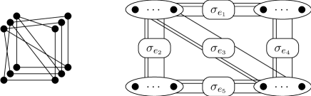
Figure 1: Top left: base graph $\mathsf{G}$. Top right: a sample of possible $2$-covers of $\mathsf{G}$. Bottom left: a possible $3$-cover of $\mathsf{G}$. Bottom right: a possible $M$-cover of $\mathsf{G}$. Here, $\sigma_{e_{1}},\ldots,\sigma_{e_{5}}$ are arbitrary edge permutations.

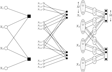
Figure 2: Left: Tanner graph $\mathsf{T}(\mathbf{H})$. Middle: a possible $3$-cover of $\mathsf{T}(\mathbf{H})$. Right: a possible $M$-cover of $\mathsf{T}(\mathbf{H})$. Here, $\{\pi_{j,i}\}_{j,i}$ are arbitrary edge permutations.

VII-A Reformulations of CC-MLD

This subsection discusses several reformulations of CC-MLD, first for general binary-input output-symmetric memoryless channels, then for the BSC. We start by repeating two reformulations of CC-MLD from Section IV.

$\displaystyle\textbf{CC-MLD1}:\quad$ minimize $\displaystyle\langle\bm{\lambda},\mathbf{x}^{\prime}\rangle$ subject to $\displaystyle\mathbf{x}^{\prime}\in\mathcal{C}_{\mathrm{CC}}.$ $\displaystyle\textbf{CC-MLD2}:\quad$ minimize $\displaystyle\langle\bm{\lambda},\mathbf{x}^{\prime}\rangle$ subject to $\displaystyle\mathbf{x}^{\prime}\in\operatorname{conv}(\mathcal{C}_{\mathrm{CC}}).$

Towards yet another reformulation of CC-MLD that we would like to present in this subsection, it is useful to introduce the hard-decision vector $\overline{\mathbf{y}}$, along with the syndrome vector $\mathbf{s}$ induced by $\overline{\mathbf{y}}$.

Definition 20

Let $\overline{\mathbf{y}}\in\mathbb{F}_{2}^{n}$ be the hard-decision vector based on the log-likelihood ratio vector $\bm{\lambda}$, namely let

$$\overline{y}_{i} \triangleq\begin{cases}0&\text{if $\lambda_{i}>0$}\\ 1&\text{if $\lambda_{i}<0$}\\ \end{cases}\quad\text{(for all $i\in\mathcal{I}$).}$$

(If $\lambda_{i}=0$, we set $\overline{y}_{i}\triangleq 0$ or $\overline{y}_{i}\triangleq 1$ according to some deterministic or random rule.) Moreover, let

$$\mathbf{s} \triangleq\mathbf{H}_{\mathrm{CC}}\cdot\overline{\mathbf{y}}\ \text{(mod $2$)}$$

be the syndrome induced by $\overline{\mathbf{y}}$. $\square$

Clearly, if the channel under consideration is a BSC with cross-over probability smaller than $1/2$ then $\overline{\mathbf{y}}=\mathbf{y}$.

With this, we have for any binary-input output-symmetric memoryless channel the following reformulation of CC-MLD in terms of $\mathbf{e}^{\prime}\triangleq\mathbf{y}-\mathbf{x}^{\prime}\ \text{(mod $2$)}$.

$\displaystyle\textbf{CC-MLD3}:\quad$ minimize $\displaystyle\lVert\bm{\lambda}_{\operatorname{supp}(\mathbf{e}^{\prime})}\rVert_{1}$ subject to $\displaystyle\mathbf{H}_{\mathrm{CC}}\cdot\mathbf{e}^{\prime}=\mathbf{s}\ \text{(mod $2$)}.$

Clearly, once the error vector estimate $\mathbf{e}^{\prime}$ is found, the codeword estimate $\mathbf{x}^{\prime}$ is obtained with the help of the expression $\mathbf{x}^{\prime}=\mathbf{y}-\mathbf{e}^{\prime}\ \text{(mod $2$)}$.

Note that for the special case of a binary-input AWGNC, this reformulation can be found, for example, in [55] or [56, Chapter 10].

Theorem 21

CC-MLD3 is a reformulation of CC-MLD1.

Proof:

See Appendix G. ∎

For a BSC we can specialize the above reformulations. Namely, for a BSC with cross-over probability $\varepsilon$, $0\leqslant\varepsilon<1/2$, we have $\lvert\lambda_{i}\rvert=L$, $i\in\mathcal{I}$, where $L\triangleq\log\bigl{(}\frac{1-\varepsilon}{\varepsilon}\bigr{)}>0$. Then, with a slight abuse of notation by employing $\lVert\,\cdot\,\rVert_{1}$ also for vectors over $\mathbb{F}_{2}$, we obtain the following reformulation.

$\displaystyle\textbf{CC-MLD4}\ \text{(BSC)}:\quad$ minimize $\displaystyle\lVert\mathbf{e}^{\prime}\rVert_{1}$ subject to $\displaystyle\mathbf{H}_{\mathrm{CC}}\cdot\mathbf{e}^{\prime}=\mathbf{s}\ \text{(mod $2$)}.$

Moreover, with a slight abuse of notation by employing $\lVert\,\cdot\,\rVert_{0}$ also for vectors over $\mathbb{F}_{2}$, CC-MLD4  (BSC) can be written as follows.

$\displaystyle\textbf{CC-MLD5}\ \text{(BSC)}:\quad$ minimize $\displaystyle\lVert\mathbf{e}^{\prime}\rVert_{0}$ subject to $\displaystyle\mathbf{H}_{\mathrm{CC}}\cdot\mathbf{e}^{\prime}=\mathbf{s}\ \text{(mod $2$)}.$

VII-B Reformulations of CC-LPD

We start by repeating the definition of CC-LPD from Section IV.

$\displaystyle\textbf{CC-LPD}:\quad$ minimize $\displaystyle\langle\bm{\lambda},\mathbf{x}^{\prime}\rangle$ subject to $\displaystyle\mathbf{x}^{\prime}\in\mathcal{P}(\mathbf{H}_{\mathrm{CC}}).$

The aim of this subsection is to discuss various reformulations of CC-LPD in terms of graph covers. In particular, the following reformulation of CC-LPD was presented in [8] and was called (blockwise) graph-cover decoding.

$\displaystyle\textbf{CC-LPD1}:\quad$ minimize $\displaystyle\frac{1}{M}\cdot\left\langle\bm{\lambda}^{\uparrow M},\mathbf{\tilde{x}}^{\prime}\right\rangle$ subject to $\displaystyle\mathbf{\tilde{H}}_{\mathrm{CC}}\cdot\mathbf{\tilde{x}}^{\prime}=\mathbf{0}^{\uparrow M}\ \text{(mod $2$)}.$

Here the minimization is over all $M\in\mathbb{Z}_{>0}$ and over all parity-check matrices $\mathbf{\tilde{H}}_{\mathrm{CC}}$ induced by all possible $M$-covers of the Tanner graph of $\mathbf{H}_{\mathrm{CC}}$.

Using the same line of reasoning as in Section VII-A, CC-LPD can be rewritten as follows.

$\displaystyle\textbf{CC-LPD2}:\quad$ minimize $\displaystyle\frac{1}{M}\cdot\lVert\bm{\lambda}^{\uparrow M}_{\operatorname{supp}(\mathbf{\tilde{e}}^{\prime})}\rVert_{1}$ subject to $\displaystyle\mathbf{\tilde{H}}_{\mathrm{CC}}\cdot\mathbf{\tilde{e}}^{\prime}=\mathbf{s}^{\uparrow M}\ \text{(mod $2$)}.$

Again, the minimization is over all $M\in\mathbb{Z}_{>0}$ and over all parity-check matrices $\mathbf{\tilde{H}}_{\mathrm{CC}}$ induced by all possible $M$-covers of the Tanner graph of $\mathbf{H}_{\mathrm{CC}}$.

For the BSC with cross-over probability $\varepsilon$, $0\leqslant\varepsilon<1/2$, we get, with a slight abuse of notation as in Section VII-A, the following specialized results.

$\displaystyle\textbf{CC-LPD3}\ \text{(BSC)}:\$ minimize $\displaystyle\frac{1}{M}\cdot\lVert\mathbf{\tilde{e}}^{\prime}\rVert_{1}$ subject to $\displaystyle\mathbf{\tilde{H}}_{\mathrm{CC}}\cdot\mathbf{\tilde{e}}^{\prime}=\mathbf{s}^{\uparrow M}\ \text{(mod $2$)}.$

$\displaystyle\textbf{CC-LPD4}\ \text{(BSC)}:\$ minimize $\displaystyle\frac{1}{M}\cdot\lVert\mathbf{\tilde{e}}^{\prime}\rVert_{0}$ subject to $\displaystyle\mathbf{\tilde{H}}_{\mathrm{CC}}\cdot\mathbf{\tilde{e}}^{\prime}=\mathbf{s}^{\uparrow M}\ \text{(mod $2$)}.$

VII-C Reformulations of CS-OPT

We start by repeating the definition of CS-OPT from Section III.

$\displaystyle\textbf{CS-OPT}:\quad$ minimize $\displaystyle\lVert\mathbf{e}^{\prime}\rVert_{0}$ subject to $\displaystyle\mathbf{H}_{\mathrm{CS}}\cdot\mathbf{e}^{\prime}=\mathbf{s}.$

Clearly, this is formally very similar to CC-MLD5 (BSC).

In order to show the tight formal relationship of CS-OPT with CC-MLD for general binary-input output-symmetric memoryless channels, in particular with respect to the reformulation CC-MLD3, we rewrite CS-OPT as follows.

$\displaystyle\textbf{CS-OPT1}:\quad$ minimize $\displaystyle\lVert\mathbf{1}_{\operatorname{supp}(\mathbf{e}^{\prime})}\rVert_{1}$ subject to $\displaystyle\mathbf{H}_{\mathrm{CS}}\cdot\mathbf{e}^{\prime}=\mathbf{s}.$

VII-D Reformulations of CS-LPD

We now come to the main part of this section, namely the reformulation of CS-LPD in terms of graph covers. We start by repeating the definition of CS-LPD from Section III.

$\displaystyle\textbf{CS-LPD}:\quad$ minimize $\displaystyle\lVert\mathbf{e}^{\prime}\rVert_{1}$ subject to $\displaystyle\mathbf{H}_{\mathrm{CS}}\cdot\mathbf{e}^{\prime}=\mathbf{s}.$

As shown in the upcoming Theorem 22, CS-LPD can be rewritten as follows.

$\displaystyle\textbf{CS-LPD1}:\quad$ minimize $\displaystyle\frac{1}{M}\cdot\lVert\mathbf{\tilde{e}}^{\prime}\rVert_{1}$ subject to $\displaystyle\mathbf{\tilde{H}}_{\mathrm{CS}}\cdot\mathbf{\tilde{e}}^{\prime}=\mathbf{s}^{\uparrow M}.$

Here the minimization is over all $M\in\mathbb{Z}_{>0}$ and over all measurement matrices $\mathbf{\tilde{H}}_{\mathrm{CS}}$ induced by all possible $M$-covers of the Tanner graph of $\mathbf{H}_{\mathrm{CS}}$.

Theorem 22

CS-LPD1 is a reformulation of CS-LPD.

Proof:

See Appendix H. ∎

Clearly, CS-LPD1 is formally very close to CC-LPD3 (BSC), thereby showing that graph covers can be used to exhibit yet another tight formal relationship between CS-LPD and CC-LPD.

Nevertheless, these graph-cover based reformulations also highlight differences between the relaxation used in the context of channel coding and the relaxation used in the context of compressed sensing.

• When relaxing CC-MLD to obtain CC-LPD, the cost function remains the same (call this property $\mathrm{P}1$) but the domain is relaxed (call this property $\mathrm{P}2$). In the graph-cover reformulations of CC-LPD, property $\mathrm{P}1$ is reflected by the fact that the cost function is a straightforward generalization of the cost function for CC-MLD. Property $\mathrm{P}2$ is reflected by the fact that in general there are feasible vectors in graph covers that cannot be explained as liftings of (convex combinations of) feasible vectors in the base graph and that, for suitable $\bm{\lambda}$-vectors, have strictly lower cost function values than any feasible vector in the base graph.

• When relaxing CS-OPT to obtain CS-LPD, the cost function is changed (call this property $\mathrm{P}1^{\prime}$), but the domain remains the same (call this property $\mathrm{P}2^{\prime}$). In the graph-cover reformulations of CS-LPD, property $\mathrm{P}1^{\prime}$ is reflected by the fact that the cost function is not a straightforward generalization of the cost function of CS-OPT. Property $\mathrm{P}2^{\prime}$ is reflected by the fact that feasible vectors in graph covers are such that they do not yield cost function values that are smaller than the cost function value of the best feasible vector in the base graph.

VIII Minimizing the Zero-Infinity Operator

For any real vector $\mathbf{a}$ we define the zero-infinity operator to be

$$\lVert\mathbf{a}\rVert_{0,\infty} \triangleq\lVert\mathbf{a}\rVert_{0}\cdot\lVert\mathbf{a}\rVert_{\infty},$$

i.e., the product of the zero norm $\lVert\mathbf{a}\rVert_{0}=|\operatorname{supp}(\mathbf{a})|$ of $\mathbf{a}$ and of the infinity norm $\lVert\mathbf{a}\rVert_{\infty}=\max_{i}|a_{i}|$ of $\mathbf{a}$. Note that for any $c\in{\mathbb{C}}$ and any real vector $\mathbf{a}$ it holds that $\lVert c\cdot\mathbf{a}\rVert_{0,\infty}=\lvert c\rvert\cdot\lVert\mathbf{a}\rVert_{0,\infty}$.

Based on this operator, in the present section we introduce $\textbf{CS-OPT}_{0,\infty}$, and we show, with the help of graph covers, that CS-LPD can not only be seen as a relaxation of CS-OPT but also as a relaxation of $\textbf{CS-OPT}_{0,\infty}$. We do this by proposing a relaxation of $\textbf{CS-OPT}_{0,\infty}$, called $\textbf{CS-REL}_{0,\infty}$, and by then showing that $\textbf{CS-REL}_{0,\infty}$ is equivalent to CS-LPD.

Moreover, we argue that the solution of CS-LPD is “closer” to the solution of $\textbf{CS-OPT}_{0,\infty}$ than the solution of CS-LPD is to the solution of CS-OPT. Note that similar to CS-OPT, the problem $\textbf{CS-OPT}_{0,\infty}$ is in general an intractable optimization problem.

One motivation for looking for different problems whose relaxations equals CS-LPD is to better understand the “strengths” and “weaknesses” of CS-LPD. In particular, if CS-LPD is the relaxation of two different problems (like CS-OPT and $\textbf{CS-OPT}_{0,\infty}$), but these two problems yield different solutions, then the solution of the relaxed problem will disagree with the solution of at least one of the two problems.

This section is structured as follows. We start by defining $\textbf{CS-OPT}_{0,\infty}$ in Section VIII-A. Then, in Section VIII-B, we discuss some geometrical aspects of $\textbf{CS-OPT}_{0,\infty}$, in particular with respect to the geometry behind CS-OPT and CS-LPD. Finally, in Section VIII-C, we introduce $\textbf{CS-REL}_{0,\infty}$ and show its equivalence to CS-LPD.

VIII-A Definition of $\textbf{CS-OPT}_{0,\infty}$

The optimization problem $\textbf{CS-OPT}_{0,\infty}$ is defined as follows.

$\displaystyle\textbf{CS-OPT}_{0,\infty}:\quad$ minimize $\displaystyle\lVert\mathbf{e}^{\prime}\rVert_{0,\infty}$ subject to $\displaystyle\mathbf{H}_{\mathrm{CS}}\cdot\mathbf{e}^{\prime}=\mathbf{s}.$

Whereas the cost function of CS-OPT, i.e., $\lVert\mathbf{e}^{\prime}\rVert_{0}$, measures the sparsity of $\mathbf{e}^{\prime}$ but not the magnitude of the elements of $\mathbf{e}^{\prime}$, the cost function of $\textbf{CS-OPT}_{0,\infty}$, i.e., $\lVert\mathbf{e}^{\prime}\rVert_{0,\infty}$, represents a trade-off between measuring the sparsity of $\mathbf{e}^{\prime}$ and measuring the largest magnitude of the components of $\mathbf{e}^{\prime}$. Clearly, in the same way that there are many good reasons to look for the vector $\mathbf{e}^{\prime}$ that minimizes the zero-norm (among all $\mathbf{e}^{\prime}$ that satisfy $\mathbf{H}_{\mathrm{CS}}\cdot\mathbf{e}^{\prime}=\mathbf{s}$), there are also many good reasons to look for the vector $\mathbf{e}^{\prime}$ that minimizes the zero-infinity operator (among all $\mathbf{e}^{\prime}$ that satisfy $\mathbf{H}_{\mathrm{CS}}\cdot\mathbf{e}^{\prime}=\mathbf{s}$). In particular, the latter is attractive when we are looking for a sparse vector $\mathbf{e}^{\prime}$ that does not have an imbalance in magnitudes between the largest component and the set of most important components.

With a slight abuse of notation, we can apply the zero-infinity operator $\lVert\,\cdot\,\rVert_{0,\infty}$ also to vectors over $\mathbb{F}_{2}$ and obtain the following reformulation of CC-MLD (BSC). (Note that for any vector $\mathbf{a}$ over $\mathbb{F}_{2}$ it holds that $\lVert\mathbf{a}\rVert_{0,\infty}=\lVert\mathbf{a}\rVert_{1}=w_{\mathrm{H}}(\mathbf{a})$.)

$\displaystyle\textbf{CC-MLD6}\ \text{(BSC)}:\quad$ minimize $\displaystyle\lVert\mathbf{e}^{\prime}\rVert_{0,\infty}$ subject to $\displaystyle\mathbf{H}_{\mathrm{CC}}\cdot\mathbf{e}^{\prime}=\mathbf{s}.$

This clearly shows that there is a close formal relationship not only between CC-MLD (BSC) and CS-OPT, but also between CC-MLD (BSC) and $\textbf{CS-OPT}_{0,\infty}$.

VIII-B Geometrical Aspects of $\textbf{CS-OPT}_{0,\infty}$

Figure 3: Unit balls for some operators. Left: $\bigl{\{}\mathbf{e}^{\prime}\in\mathbb{R}^{2}\bigm{|}\lVert\mathbf{e}^{\prime}\rVert_{0}\leqslant 1\bigr{\}}$. Middle: $\bigl{\{}\mathbf{e}^{\prime}\in\mathbb{R}^{2}\bigm{|}\lVert\mathbf{e}^{\prime}\rVert_{0,\infty}\leqslant 1\bigr{\}}$. Right: $\bigl{\{}\mathbf{e}^{\prime}\in\mathbb{R}^{2}\bigm{|}\lVert\mathbf{e}^{\prime}\rVert_{1}\leqslant 1\bigr{\}}$.

We want to discuss some geometrical aspects of CS-OPT, $\textbf{CS-OPT}_{0,\infty}$, and CS-LPD. Namely, as is well known, CS-OPT can be formulated as finding the smallest $\ell_{0}$-norm ball of radius $r$ (cf. Figure 3 (left)) that intersects the set $\bigl{\{}\mathbf{e}^{\prime}\bigm{|}\mathbf{H}_{\mathrm{CS}}\cdot\mathbf{e}^{\prime}=\mathbf{s}\bigr{\}}$, and in the same spirit, CS-LPD can be formulated as finding the smallest $\ell_{1}$-norm ball of radius $r$ (cf. Figure 3 (right)) that intersects with the set $\bigl{\{}\mathbf{e}^{\prime}\bigm{|}\mathbf{H}_{\mathrm{CS}}\cdot\mathbf{e}^{\prime}=\mathbf{s}\bigr{\}}$. Clearly, the fact that CS-OPT and CS-LPD can yield different solutions stems from the fact that these balls have different shapes. Of course, the success of CS-LPD is a consequence of the fact that, nevertheless, under suitable conditions, the solution given by the $\ell_{1}$-norm ball is (nearly) the same as the solution given by the $\ell_{0}$-norm ball.

In the same vein, $\textbf{CS-OPT}_{0,\infty}$ can be formulated as finding the smallest zero-infinity-operator ball of radius $r$ (cf. Figure 3 (middle)) that intersects the set $\bigl{\{}\mathbf{e}^{\prime}\bigm{|}\mathbf{H}_{\mathrm{CS}}\cdot\mathbf{e}^{\prime}=\mathbf{s}\bigr{\}}$. As it can be seen from Figure 3, the zero-infinity-operator unit ball is closer in shape to the $\ell_{1}$-norm unit ball than the $\ell_{0}$-norm unit ball is to the $\ell_{1}$-norm unit ball. Therefore, we expect that the solution given by CS-LPD is “closer” to the solution given by $\textbf{CS-OPT}_{0,\infty}$ than the solution of CS-LPD is to the solution given by CS-OPT. In that sense, $\textbf{CS-OPT}_{0,\infty}$ is at least as justifiably as CS-OPT a difficult optimization problem whose solution is approximated by CS-LPD.

VIII-C Relaxation of $\textbf{CS-OPT}_{0,\infty}$

In this subsection we introduce $\textbf{CS-REL}_{0,\infty}$ as a relaxation of $\textbf{CS-OPT}_{0,\infty}$; the main result will be that $\textbf{CS-REL}_{0,\infty}$ equals CS-LPD. Our results will be formulated in terms of graph covers, we therefore use the graph-cover related notation that was introduced in Section VII, along with the mapping $\bm{\varphi}_{M}$ that was defined in Section II.

In order to motivate the formulation of $\textbf{CS-REL}_{0,\infty}$, we first present a reformulation of CC-LPD (BSC). Namely, CC-LPD3 (BSC) or CC-LPD4 (BSC) from Section VII-B can be rewritten as follows.

$\displaystyle\textbf{CC-LPD5}\ \text{(BSC)}:\$ minimize $\displaystyle\frac{1}{M}\cdot\lVert\mathbf{\tilde{e}}^{\prime}\rVert_{0,\infty}$ subject to $\displaystyle\mathbf{\tilde{H}}_{\mathrm{CC}}\cdot\mathbf{\tilde{e}}^{\prime}=\mathbf{s}^{\uparrow M}\ \text{(mod $2$)}.$

Then, because for any vector $\mathbf{\tilde{s}}\in\mathbb{F}_{2}^{|\mathcal{J}|\cdot M}$ it holds that $\bm{\varphi}_{M}(\mathbf{\tilde{s}})=\mathbf{s}$ if and only if $\mathbf{\tilde{s}}=\mathbf{s}^{\uparrow M}$, CC-LPD5 (BSC) can also be written as follows.

$\displaystyle\textbf{CC-LPD6}\ \text{(BSC)}:\quad$ minimize $\displaystyle\frac{1}{M}\cdot\lVert\mathbf{\tilde{e}}^{\prime}\rVert_{0,\infty}$ subject to $\displaystyle\mathbf{\tilde{H}}_{\mathrm{CC}}\cdot\mathbf{\tilde{e}}^{\prime}=\mathbf{\tilde{s}}\ \text{(mod $2$)}$ $\displaystyle\hskip 7.82433pt\bm{\varphi}_{M}(\mathbf{\tilde{s}})=\mathbf{s}.$

The transition that leads from CC-MLD to its relaxation CC-LPD6 (BSC) inspires a relaxation of $\textbf{CS-OPT}_{0,\infty}$ as follows.

$\displaystyle\textbf{CS-REL}_{0,\infty}:\quad$ minimize $\displaystyle\frac{1}{M}\cdot\lVert\mathbf{\tilde{e}}^{\prime}\rVert_{0,\infty}$ subject to $\displaystyle\mathbf{\tilde{H}}_{\mathrm{CS}}\cdot\mathbf{\tilde{e}}^{\prime}=\mathbf{\tilde{s}}$ $\displaystyle\hskip 6.82881pt\bm{\varphi}_{M}(\mathbf{\tilde{s}})=\mathbf{s}.$

Here the minimization is over all $M\in\mathbb{Z}_{>0}$ and over all measurement matrices $\mathbf{\tilde{H}}_{\mathrm{CS}}$ induced by all possible $M$-covers of the Tanner graph of $\mathbf{H}_{\mathrm{CS}}$. Note that, in contrast to CC-LPD6 (BSC), in general the optimal solution $(\mathbf{\tilde{e}},\mathbf{\tilde{s}})$ of $\textbf{CS-REL}_{0,\infty}$ does not satisfy $\mathbf{\tilde{s}}=\mathbf{s}^{\uparrow M}$.

Towards establishing the equivalence of $\textbf{CS-REL}_{0,\infty}$ and CS-LPD, the following simple lemma will prove to be useful.

Lemma 23

For any real vector $\mathbf{a}$ it holds that

$$\lVert\mathbf{a}\rVert_{1} \leqslant\lVert\mathbf{a}\rVert_{0,\infty},$$

with equality if and only if all non-zero components of $\mathbf{a}$ have the same absolute value.

Proof:

The proof of this lemma is straightforward. ∎

Theorem 24

Let $\mathbf{H}_{\mathrm{CS}}$ be a measurement matrix over the reals with entries equal to zero, one, and minus one. For syndrome vectors $\mathbf{s}$ that have only rational components, CS-LPD and $\textbf{CS-REL}_{0,\infty}$ are equivalent in the sense that there is an optimal $\mathbf{e}^{\prime}$ in CS-LPD and an optimal $\mathbf{\tilde{e}}^{\prime}$ in $\textbf{CS-REL}_{0,\infty}$ such that $\mathbf{e}^{\prime}=\bm{\varphi}_{M}(\mathbf{\tilde{e}}^{\prime})$.

Proof:

See Appendix I. ∎

IX Conclusions and Outlook

In this paper we have established a mathematical connection between channel coding and compressed sensing LP relaxations. The key observation, in its simplest version, was that points in the nullspace of a zero-one matrix (considered over the reals) can be mapped to points in the fundamental cone of the same matrix (considered as the parity-check matrix of a code over $\mathbb{F}_{2}$). This allowed us to show, among other results, that parity-check matrices of “good” channel codes can be used as provably “good” measurement matrices under basis pursuit.

Let us comment on a variety of topics.

• In addition to CS-LPD, a number of combinatorial algorithms (e.g. [57, 31, 32, 35, 11, 58]) have been proposed for compressed sensing problems, with the benefit of faster decoding complexity and comparable performance to CS-LPD. It would be interesting to investigate if the connection of sparse recovery problems to channel coding extends in a similar manner for these decoders. One example of such a clear connection is the bit-flipping algorithm of Sipser and Spielman [39] and the corresponding algorithm for compressed sensing by Xu and Hassibi [31]. Channel-coding-inspired message-passing decoders for compressed sensing problems were also recently discussed in [59, 37, 38, 60, 61].

• An interesting research direction is to use optimized LDPC matrices (see, e.g. [23]) to create measurement matrices. There is a large body of channel coding work that could be transferable to the measurement matrix design problem.

  In this context, an important theoretical question is related to being able to certify in polynomial time that a given measurement matrix has “good” performance. To the best of our knowledge, our results form the first known case where girth, an efficiently checkable property, can be used as a certificate of goodness of a measurement matrix. It is possible that girth can be used to establish a success witness for CS-LPD directly, and this would be an interesting direction for future research.

• One important research direction in compressed sensing involves dealing with noisy measurements. This problem can still be addressed with $\ell_{1}$ minimization (see, e.g., [62]) and also with less complex signal reconstruction algorithms (see, e.g., [63]). It would be very interesting to investigate if our nullspace connections can be extended to a coding theory result equivalent to noisy compressed sensing.

• Beyond channel coding problems, the LP relaxation of [6] is a special case of a relaxation of the marginal polytope for general graphical models. One very interesting research direction is to explore if the connection we have established between CS-LPD and CC-LPD is also just a special case of a more general theory.

• We have also discussed various reformulations of the optimization problems under investigation. This leads to a strengthening of the ties between some of the optimization problems. Moreover, we have introduced the zero-infinity operator optimization problem $\textbf{CS-OPT}_{0,\infty}$, an optimization problem with the property that the solution of CS-LPD can be considered to be at least as good an approximation of the solution of $\textbf{CS-OPT}_{0,\infty}$ as the solution of CS-LPD is an approximation of the solution of CS-OPT. We leave it as an open question if the results and observations of Section VIII can be generalized for more general matrices or specific families of signals (like non-negative sparse signals as in [64, 65]).

Appendix A Proof of Theorem 5

Suppose that $\mathbf{H}_{\mathrm{CS}}$ has the claimed nullspace property. Since $\mathbf{H}_{\mathrm{CS}}\cdot\mathbf{e}=\mathbf{s}$ and $\mathbf{H}_{\mathrm{CS}}\cdot\mathbf{\hat{e}}=\mathbf{s}$, it easily follows that $\bm{\nu}\triangleq\mathbf{e}-\mathbf{\hat{e}}$ is in the nullspace of $\mathbf{H}_{\mathrm{CS}}$. So,

$$\lVert\mathbf{e}_{\mathcal{S}}\rVert_{1}+\lVert\mathbf{e}_{\overline{\mathcal{S}}}\rVert_{1} =\lVert\mathbf{e}\rVert_{1}$$

$$\overset{\text{(a)}}{\geqslant}\lVert\mathbf{\hat{e}}\rVert_{1}$$

$$=\lVert\mathbf{e}-\bm{\nu}\rVert_{1}$$

$$=\lVert\mathbf{e}_{\mathcal{S}}-\bm{\nu}_{\mathcal{S}}\rVert_{1}+\lVert\mathbf{e}_{\overline{\mathcal{S}}}-\bm{\nu}_{\overline{\mathcal{S}}}\rVert_{1}$$

$$\overset{\text{(b)}}{\geqslant}\lVert\mathbf{e}_{\mathcal{S}}\rVert_{1}-\lVert\bm{\nu}_{\mathcal{S}}\rVert_{1}+\lVert\bm{\nu}_{\overline{\mathcal{S}}}\rVert_{1}-\lVert\mathbf{e}_{\overline{\mathcal{S}}}\rVert_{1}$$

$$\overset{\text{(c)}}{\geqslant}\lVert\mathbf{e}_{\mathcal{S}}\rVert_{1}+\frac{C-1}{C+1}\cdot\lVert\bm{\nu}\rVert_{1}-\lVert\mathbf{e}_{\overline{\mathcal{S}}}\rVert_{1},$$ (5)

where step (a) follows from the fact that the solution of CS-LPD satisfies $\lVert\mathbf{\hat{e}}\rVert_{1}\leqslant\lVert\mathbf{e}\rVert_{1}$, where step (b) follows from applying the triangle inequality property of the $\ell_{1}$-norm twice, and where step (c) follows from

$$-\lVert\bm{\nu}_{\mathcal{S}}\rVert_{1}+\lVert\bm{\nu}_{\overline{\mathcal{S}}}\rVert_{1} \overset{\text{(d)}}{\geqslant}\frac{C-1}{C+1}\cdot\lVert\bm{\nu}\rVert_{1}.$$

Here, step (d) is a consequence of

$$(C\!+\!1)\,\cdot\, \big{(}-\lVert\bm{\nu}_{\mathcal{S}}\rVert_{1}+\lVert\bm{\nu}_{\overline{\mathcal{S}}}\rVert_{1}\big{)}$$

$$=-C\cdot\lVert\bm{\nu}_{\mathcal{S}}\rVert_{1}-\lVert\bm{\nu}_{\mathcal{S}}\rVert_{1}+C\cdot\lVert\bm{\nu}_{\overline{\mathcal{S}}}\rVert_{1}+\lVert\bm{\nu}_{\overline{\mathcal{S}}}\rVert_{1}$$

$$\overset{\text{(e)}}{\geqslant}-\lVert\bm{\nu}_{\overline{\mathcal{S}}}\rVert_{1}-\lVert\bm{\nu}_{\mathcal{S}}\rVert_{1}+C\cdot\lVert\bm{\nu}_{\overline{\mathcal{S}}}\rVert_{1}+C\cdot\lVert\bm{\nu}_{\mathcal{S}}\rVert_{1}$$

$$=(C\!-\!1)\cdot\lVert\bm{\nu}_{\mathcal{S}}\rVert_{1}+(C\!-\!1)\cdot\lVert\bm{\nu}_{\overline{\mathcal{S}}}\rVert_{1}$$

$$=(C\!-\!1)\cdot\lVert\bm{\nu}\rVert_{1},$$

where step (e) follows from applying twice the fact that $\bm{\nu}\in\operatorname{Nullsp}_{\mathbb{R}}(\mathbf{H}_{\mathrm{CS}})$ and the assumption that $\mathbf{H}_{\mathrm{CS}}\in\mathrm{NSP}^{\leqslant}_{\mathbb{R}}(k,C)$. Subtracting the term $\lVert\mathbf{e}_{\mathcal{S}}\rVert_{1}$ on both sides of (5), and solving for $\lVert\bm{\nu}\rVert_{1}=\lVert\mathbf{e}-\mathbf{\hat{e}}\rVert_{1}$ yields the promised result.

Appendix B Proof of Lemma 8

Without loss of generality, we can assume that the all-zero codeword was transmitted. Let $+L>0$ be the log-likelihood ratio associated with a received $0$, and let $-L<0$ be the log-likelihood ratio associated with a received $1$. Therefore, $\lambda_{i}=+L$ if $i\in\overline{\mathcal{S}}$ and $\lambda_{i}=-L$ if $i\in\mathcal{S}$. Then it follows from the assumptions in the lemma statement that for any $\bm{\omega}\in\mathcal{K}(\mathbf{H}_{\mathrm{CC}})\setminus\{\mathbf{0}\}$ it holds that

$$\langle\bm{\lambda},\bm{\omega}\rangle =\sum_{i\in\overline{\mathcal{S}}}(+L)\cdot\omega_{i}+\sum_{i\in\mathcal{S}}(-L)\cdot\omega_{i}$$

$$\overset{\text{(a)}}{=}L\cdot\lVert\bm{\omega}_{\overline{\mathcal{S}}}\rVert_{1}-L\cdot\lVert\bm{\omega}_{\mathcal{S}}\rVert_{1}\overset{\text{(b)}}{>}0=\langle\bm{\lambda},\mathbf{0}\rangle,$$

where step (a) follows from the fact that $|\omega_{i}|=\omega_{i}$ for all $i\in\mathcal{I}(\mathbf{H}_{\mathrm{CC}})$, and where step (b) follows from (4). Therefore, under CC-LPD the all-zero codeword has the lowest cost function value when compared to all non-zero pseudo-codewords in the fundamental cone, and therefore also compared to all non-zero pseudo-codewords in the fundamental polytope.

Appendix C Proof of Lemma 10

Case 1: Let $|\mathcal{S}|<\frac{1}{2}\cdot w_{\mathrm{p}}^{\mathrm{BSC}}(\bm{\omega})$. The proof is by contradiction: assume that $\lVert\bm{\omega}_{\mathcal{S}}\rVert_{1}\geqslant\lVert\bm{\omega}_{\overline{\mathcal{S}}}\rVert_{1}$. This statement is clearly equivalent to the statement that $2\cdot\lVert\bm{\omega}_{\mathcal{S}}\rVert_{1}\geqslant\lVert\bm{\omega}_{\mathcal{S}}\rVert_{1}+\lVert\bm{\omega}_{\overline{\mathcal{S}}}\rVert_{1}=\lVert\bm{\omega}\rVert_{1}$, which is equivalent to the statement that $\lVert\bm{\omega}_{\mathcal{S}}\rVert_{1}\geqslant\frac{1}{2}\cdot\lVert\bm{\omega}\rVert_{1}$. In terms of the notation in Definition 9, this means that

$$w_{\mathrm{p}}^{\mathrm{BSC}}(\bm{\omega}) =2\cdot F^{-1}\left(\frac{\lVert\bm{\omega}\rVert_{1}}{2}\right)\overset{\text{(a)}}{\leqslant}2\cdot F^{-1}(\lVert\bm{\omega}_{\mathcal{S}}\rVert_{1})$$

$$\overset{\text{(b)}}{\leqslant}2\cdot\frac{\lVert\bm{\omega}_{\mathcal{S}}\rVert_{1}}{\lVert\bm{\omega}\rVert_{\infty}}\leqslant 2\cdot\frac{|\mathcal{S}|\cdot\lVert\bm{\omega}\rVert_{\infty}}{\lVert\bm{\omega}\rVert_{\infty}}=2\cdot|\mathcal{S}|,$$

where at step (a) we have used the fact that $F^{-1}$ is a (strictly) non-decreasing function and where at step (b) we have used the fact that the slope of $F^{-1}$ (over the domain where $F^{-1}$ is defined) is at least $1/\lVert\bm{\omega}\rVert_{\infty}$. The obtained inequality, however, is a contradiction to the assumption that $|\mathcal{S}|<\frac{1}{2}\cdot w_{\mathrm{p}}^{\mathrm{BSC}}(\bm{\omega})$.

Case 2: Let $|\mathcal{S}|<\frac{1}{2}\cdot w_{\mathrm{p}}^{\mathrm{BSC}^{\prime}}(\bm{\omega})$. The proof is by contradiction: assume that $\lVert\bm{\omega}_{\mathcal{S}}\rVert_{1}\geqslant\lVert\bm{\omega}_{\overline{\mathcal{S}}}\rVert_{1}$. Then, using the definition of $\bm{\omega}^{\prime}$ based on $\bm{\omega}$ (cf. Section IV-C), we obtain

$$\lVert\bm{\omega}^{\prime}_{\{1,\ldots,|\mathcal{S}|\}}\rVert_{1} \,\geqslant\,\lVert\bm{\omega}_{\mathcal{S}}\rVert_{1}\,\geqslant\,\lVert\bm{\omega}_{\overline{\mathcal{S}}}\rVert_{1}\,\geqslant\,\lVert\bm{\omega}^{\prime}_{\{|\mathcal{S}|+1,\ldots,n\}}\rVert_{1}.$$

If $w_{\mathrm{p}}^{\mathrm{BSC}^{\prime}}(\bm{\omega})$ is an even integer, then the above line of inequalities shows that $|\mathcal{S}|\geqslant\frac{1}{2}\cdot w_{\mathrm{p}}^{\mathrm{BSC}^{\prime}}(\bm{\omega})$, which is a contradiction to the assumption that $|\mathcal{S}|<\frac{1}{2}\cdot w_{\mathrm{p}}^{\mathrm{BSC}^{\prime}}(\bm{\omega})$. If $w_{\mathrm{p}}^{\mathrm{BSC}^{\prime}}(\bm{\omega})$ is an odd integer, then the above line of inequalities shows that $|\mathcal{S}|\geqslant\frac{1}{2}\cdot\bigl{(}w_{\mathrm{p}}^{\mathrm{BSC}^{\prime}}(\bm{\omega})+1\bigr{)}>\frac{1}{2}w_{\mathrm{p}}^{\mathrm{BSC}^{\prime}}(\bm{\omega})$, which again is a contradiction to the assumption that $|\mathcal{S}|<\frac{1}{2}\cdot w_{\mathrm{p}}^{\mathrm{BSC}^{\prime}}(\bm{\omega})$.

Appendix D Extensions of the Bridge Lemma

The aim of this appendix is to extend Lemma 11 (cf. Section V) to measurement matrices beyond zero-one matrices. In that vein we will present three generalizations in Lemmas 25, 29, and 31. Note that the setup in this appendix will be slightly more general than the compressed sensing setup in Section III (and in most of the rest of this paper). In particular, we allow matrices and vectors to be over ${\mathbb{C}}$, and not just over $\mathbb{R}$.

We will need some additional notation. Namely, similarly to the way that we have extended the absolute value operator $\lvert\,\cdot\,\rvert$ from scalars to vectors at the beginning of Section V, we will now extend its use from scalars to matrices.

Moreover, we let $\left\lvert\,\cdot\,\right\rvert_{*}$ be an arbitrary norm for the complex numbers. As such, $\left\lvert\,\cdot\,\right\rvert_{*}$ satisfies for any $a,b,c\in{\mathbb{C}}$ the triangle inequality $\left\lvert a+b\right\rvert_{*}\leqslant\left\lvert a\right\rvert_{*}+\left\lvert b\right\rvert_{*}$ and the equality $\left\lvert c\cdot a\right\rvert_{*}=\lvert c\rvert\cdot\left\lvert a\right\rvert_{*}$. In the same way the absolute value operator $\lvert\,\cdot\,\rvert$ was extended from scalars to vectors and matrices, we extend the norm operator $\left\lvert\,\cdot\,\right\rvert_{*}$ from scalars to vectors and matrices.

We let $\left\lVert\,\cdot\,\right\rVert_{*}$ be an arbitrary vector norm for complex vectors that reduces to $\left\lvert\,\cdot\,\right\rvert_{*}$ for vectors with one component. As such, $\left\lVert\,\cdot\,\right\rVert_{*}$ satisfies for any $c\in{\mathbb{C}}$ and any complex vectors $\mathbf{a}$ and $\mathbf{b}$ with the same number of components the triangle inequality $\left\lVert\mathbf{a}+\mathbf{b}\right\rVert_{*}\leqslant\left\lVert\mathbf{a}\right\rVert_{*}+\left\lVert\mathbf{b}\right\rVert_{*}$ and the equality $\left\lVert c\cdot\mathbf{a}\right\rVert_{*}=\lvert c\rvert\cdot\left\lVert\mathbf{a}\right\rVert_{*}$.

We are now ready to discuss our first extension of Lemma 11, which generalizes the setup of that lemma from real measurement matrices where every entry is equal to either zero or one to complex measurement matrices where the absolute value of every entry is equal to either zero or one. Note that the upcoming lemma also generalizes the mapping that is applied to the vectors in the nullspace of the measurement matrix.

Lemma 25

Let $\mathbf{H}_{\mathrm{CS}}=(h_{j,i})_{j,i}$ be a measurement matrix over ${\mathbb{C}}$ such that $\lvert h_{j,i}\rvert\in\{0,1\}$ for all $(j,i)\in\mathcal{J}(\mathbf{H}_{\mathrm{CS}})\times\mathcal{I}(\mathbf{H}_{\mathrm{CS}})$, and let $\left\lvert\,\cdot\,\right\rvert_{*}$ be an arbitrary norm on ${\mathbb{C}}$. Then

$$\bm{\nu}\in\operatorname{Nullsp}_{{\mathbb{C}}}(\mathbf{H}_{\mathrm{CS}})\ \ \ \Rightarrow\ \ \ \left\lvert\bm{\nu}\right\rvert_{*}\in\mathcal{K}\big{(}\lvert\mathbf{H}_{\mathrm{CS}}\rvert\big{)}.$$

Remark: Note that $\operatorname{supp}(\bm{\nu})=\operatorname{supp}(\left\lvert\bm{\nu}\right\rvert_{*})$.

Proof:

Let $\bm{\omega}\triangleq\left\lvert\bm{\nu}\right\rvert_{*}$. In order to show that such a vector $\bm{\omega}$ is indeed in the fundamental cone of $\lvert\mathbf{H}_{\mathrm{CS}}\rvert$, we need to verify (2) and (3). The way $\bm{\omega}$ is defined, it is clear that it satisfies (2). Therefore, let us focus on the proof that $\bm{\omega}$ satisfies (3). Namely, from $\bm{\nu}\in\operatorname{Nullsp}_{{\mathbb{C}}}(\mathbf{H}_{\mathrm{CS}})$ it follows that for all $j\in\mathcal{J}$, $\sum_{i\in\mathcal{I}}h_{j,i}\nu_{i}=0$. For all $j\in\mathcal{J}$ and all $i\in\mathcal{I}_{j}$ this implies that

$$\omega_{i} =\left\lvert\nu_{i}\right\rvert_{*}=\lvert h_{j,i}\rvert\cdot\left\lvert\nu_{i}\right\rvert_{*}=\left\lvert h_{j,i}\nu_{i}\right\rvert_{*}=\left\lvert\,\,-\!\!\sum_{i^{\prime}\in\mathcal{I}\setminus i}h_{j,i^{\prime}}\nu_{i^{\prime}}\right\rvert_{*}$$

$$\leqslant\sum_{i^{\prime}\in\mathcal{I}\setminus i}\left\lvert h_{j,i^{\prime}}\nu_{i^{\prime}}\right\rvert_{*}=\sum_{i^{\prime}\in\mathcal{I}\setminus i}\lvert h_{j,i^{\prime}}\rvert\cdot\left\lvert\nu_{i^{\prime}}\right\rvert_{*}=\sum_{i^{\prime}\in\mathcal{I}_{j}\setminus i}\left\lvert\nu_{i^{\prime}}\right\rvert_{*}$$

$$=\sum_{i^{\prime}\in\mathcal{I}_{j}\setminus i}\omega_{i^{\prime}},$$

showing that $\bm{\omega}$ indeed satisfies (3). ∎

Example 26

The measurement matrix

$$\mathbf{H}_{\mathrm{CS}} \triangleq\begin{pmatrix}1&0&\frac{1}{\sqrt{2}}(1+i)\\ -1&i&1\end{pmatrix}$$

satisfies

$$\lvert\mathbf{H}_{\mathrm{CS}}\rvert =\begin{pmatrix}1&0&1\\ 1&1&1\end{pmatrix},$$

and so Lemma 25 is applicable. An example of a vector in $\operatorname{Nullsp}_{{\mathbb{C}}}(\mathbf{H}_{\mathrm{CS}})$ is

$$\bm{\nu} \triangleq\left(\frac{1}{\sqrt{2}}(1+i),\ \frac{1}{\sqrt{2}}-i\left(1+\frac{1}{\sqrt{2}}\right),\ -1\right).$$

Choosing $\left\lvert\,\cdot\,\right\rvert_{*}\triangleq\lvert\,\cdot\,\rvert$, we obtain

$$\left\lvert\bm{\nu}\right\rvert_{*} =\left(1,\ \sqrt{2+\sqrt{2}},\ 1\right)=\left(1,\ 1.848...,\ 1\right)\in\mathcal{K}\big{(}\lvert\mathbf{H}_{\mathrm{CS}}\rvert\big{)}.$$

$\square$

The second extension of Lemma 11 generalizes that lemma to hold also for complex measurement matrices where the absolute value of every entry is an integer. In order to present this lemma, we need the following definition, which is subsequently illustrated by Example 28.

Definition 27

Let $\mathbf{H}_{\mathrm{CS}}=(h_{j,i})_{j,i}$ be a measurement matrix over ${\mathbb{C}}$ such that $\lvert h_{j,i}\rvert\in\mathbb{Z}_{\geqslant 0}$ for all $(j,i)\in\mathcal{J}(\mathbf{H}_{\mathrm{CS}})\times\mathcal{I}(\mathbf{H}_{\mathrm{CS}})$, and let $M\in\mathbb{Z}_{>0}$ be such that $M\geqslant\max_{(j,i)}\,\lvert h_{j,i}\rvert$. We define an $M$-fold cover $\mathbf{\tilde{H}}_{\mathrm{CS}}$ of $\mathbf{H}_{\mathrm{CS}}$ as follows: for $(j,i)\in\mathcal{J}(\mathbf{H}_{\mathrm{CS}})\times\mathcal{I}(\mathbf{H}_{\mathrm{CS}})$, if the scalar $h_{j,i}$ is non-zero then it is replaced by a matrix, namely $h_{j,i}/\lvert h_{j,i}\rvert$ times the sum of $\lvert h_{j,i}\rvert$ arbitrary $M\times M$ permutation matrices with non-overlapping support. However, if $h_{j,i}=0$ then the scalar $h_{j,i}$ is replaced by an all-zero matrix of size $M\times M$. $\square$

Note that all entries of the matrix $\mathbf{\tilde{H}}_{\mathrm{CS}}$ in Definition 27 have absolute value equal to either zero or one.

Example 28

Let

$$\mathbf{H}_{\mathrm{CS}} \triangleq\begin{pmatrix}1&0&\sqrt{2}(1+i)\\ -2&i&3\end{pmatrix}.$$

Clearly

$$\lvert\mathbf{H}_{\mathrm{CS}}\rvert =\begin{pmatrix}1&0&2\\ 2&1&3\end{pmatrix},$$

and so, choosing $M\triangleq 3$ and

$$\mathbf{\tilde{H}}_{\mathrm{CS}} \triangleq\left(\begin{array}[]{ccc|ccc|ccc}0&1&0&0&0&0&\frac{1+i}{\sqrt{2}}&\frac{1+i}{\sqrt{2}}&0\\ 1&0&0&0&0&0&\frac{1+i}{\sqrt{2}}&0&\frac{1+i}{\sqrt{2}}\\ 0&0&1&0&0&0&0&\frac{1+i}{\sqrt{2}}&\frac{1+i}{\sqrt{2}}\\ \hline\cr 0&-1&-1&i&0&0&1&1&1\\ -1&-1&0&0&i&0&1&1&1\\ -1&0&-1&0&0&i&1&1&1\\ \end{array}\right),$$

we obtain a matrix described by the procedure of Definition 27. $\square$

Lemma 29

Let $\mathbf{H}_{\mathrm{CS}}=(h_{j,i})_{j,i}$ be a measurement matrix over ${\mathbb{C}}$ such that $\lvert h_{j,i}\rvert\in\mathbb{Z}_{\geqslant 0}$ for all $(j,i)\in\mathcal{J}(\mathbf{H}_{\mathrm{CS}})\times\mathcal{I}(\mathbf{H}_{\mathrm{CS}})$. Let $M\in\mathbb{Z}_{>0}$ be such that $M\geqslant\max_{(j,i)}\,\lvert h_{j,i}\rvert$, and let $\mathbf{\tilde{H}}_{\mathrm{CS}}$ be a matrix obtained by the procedure in Definition 27. Moreover, let $\left\lvert\,\cdot\,\right\rvert_{*}$ be an arbitrary norm on ${\mathbb{C}}$. Then

$$\bm{\nu}\in\operatorname{Nullsp}_{{\mathbb{C}}}(\mathbf{H}_{\mathrm{CS}}) \ \ \ \Rightarrow\ \ \ \bm{\nu}^{\uparrow M}\in\operatorname{Nullsp}_{{\mathbb{C}}}(\mathbf{\tilde{H}}_{\mathrm{CS}})$$

$$\ \ \ \Rightarrow\ \ \ \left\lvert\bm{\nu}^{\uparrow M}\right\rvert_{*}\in\mathcal{K}\big{(}\lvert\mathbf{\tilde{H}}_{\mathrm{CS}}\rvert\big{)}.$$

Additionally, with respect to the first implication sign we have the following converse: for any $\bm{\tilde{\nu}}\in{\mathbb{C}}^{Mn}$ we have

$$\bm{\varphi}_{M}(\bm{\tilde{\nu}})\in\operatorname{Nullsp}_{{\mathbb{C}}}(\mathbf{H}_{\mathrm{CS}}) \ \ \ \Leftarrow\ \ \ \bm{\tilde{\nu}}\in\operatorname{Nullsp}_{{\mathbb{C}}}(\mathbf{\tilde{H}}_{\mathrm{CS}}).$$

Proof:

Let $\mathbf{\tilde{H}}_{\mathrm{CS}}=(\tilde{h}_{(j,m^{\prime}),(i,m)})_{(j,m^{\prime}),(i,m)}$. Note that by the construction in Definition 27, it holds that

$$\sum_{m^{\prime}\in\mathcal{[}M]}\tilde{h}_{(j,m^{\prime}),(i,m)} =h_{j,i}\ \ \text{for any $(j,i,m)\in\mathcal{J}\!\times\!\mathcal{I}\!\times\![M]$},$$

$$\sum_{m\in\mathcal{[}M]}\tilde{h}_{(j,m^{\prime}),(i,m)} =h_{j,i}\ \ \text{for any $(j,m^{\prime},i)\in\mathcal{J}\!\times\![M]\!\times\!\mathcal{I}$}.$$

Let $\bm{\nu}\in\operatorname{Nullsp}_{{\mathbb{C}}}(\mathbf{H}_{\mathrm{CS}})$. Then, for every $(j,m^{\prime})\in\mathcal{J}\times[M]$ we have

$$\sum_{(i,m)\in\mathcal{I}\times\mathcal{[}M]}\!\!\!\tilde{h}_{(j,m^{\prime}),(i,m)}\nu^{\uparrow M}_{(i,m)}=\sum_{(i,m)\in\mathcal{I}\times\mathcal{[}M]}\!\!\!\tilde{h}_{(j,m^{\prime}),(i,m)}\nu_{i}$$

$$\quad\quad=\sum_{i\in\mathcal{I}}\nu_{i}\sum_{m\in\mathcal{[}M]}\tilde{h}_{(j,m^{\prime}),(i,m)}=\sum_{i\in\mathcal{I}}\nu_{i}h_{j,i}=0,$$

where the last equality follows from the assumption that $\bm{\nu}\in\operatorname{Nullsp}_{{\mathbb{C}}}(\mathbf{H}_{\mathrm{CS}})$. Therefore $\bm{\nu}^{\uparrow M}\in\operatorname{Nullsp}_{{\mathbb{C}}}(\mathbf{\tilde{H}}_{\mathrm{CS}})$. Because $\lvert\tilde{h}_{(j,m^{\prime}),(i,m)}\rvert\in\{0,1\}$ for all $(j,m^{\prime},i,m)\in\mathcal{J}\times[M]\times\mathcal{I}\times[M]$, we can then apply Lemma 25 to conclude that $\left\lvert\bm{\nu}^{\uparrow M}\right\rvert_{*}\in\mathcal{K}\big{(}\lvert\mathbf{\tilde{H}}_{\mathrm{CS}}\rvert\big{)}$.

Now, in order to prove the last part of the lemma, assume that $\bm{\tilde{\nu}}\in\operatorname{Nullsp}_{{\mathbb{C}}}(\mathbf{\tilde{H}}_{\mathrm{CS}})$ and define $\bm{\nu}\triangleq\bm{\varphi}_{M}(\bm{\tilde{\nu}})$. Then for every $j\in\mathcal{J}$ we have

$$\sum_{i\in\mathcal{I}}h_{j,i}\nu_{i} =\sum_{i\in\mathcal{I}}h_{j,i}\cdot\frac{1}{M}\sum_{m\in[M]}\tilde{\nu}_{(i,m)}$$

$$=\frac{1}{M}\sum_{i\in\mathcal{I}}\sum_{m\in[M]}h_{j,i}\cdot\tilde{\nu}_{(i,m)}$$

$$=\frac{1}{M}\sum_{i\in\mathcal{I}}\sum_{m\in[M]}\sum_{m^{\prime}\in[M]}\tilde{h}_{(j,m^{\prime}),(i,m)}\cdot\tilde{\nu}_{(i,m)}$$

$$=\frac{1}{M}\sum_{m^{\prime}\in[M]}\left(\sum_{i\in\mathcal{I}}\sum_{m\in[M]}\tilde{h}_{(j,m^{\prime}),(i,m)}\cdot\tilde{\nu}_{(i,m)}\right)$$

$$=0,$$

where the last equality follows from the assumption that $\bm{\tilde{\nu}}\in\operatorname{Nullsp}_{{\mathbb{C}}}(\mathbf{\tilde{H}}_{\mathrm{CS}})$, i.e., for every $(j,m^{\prime})\in\mathcal{J}\times[M]$ the expression in parentheses equals zero. Therefore, $\bm{\nu}=\bm{\varphi}_{M}(\bm{\tilde{\nu}})\in\operatorname{Nullsp}_{{\mathbb{C}}}(\mathbf{H}_{\mathrm{CS}})$. ∎

Example 30

Consider the measurement matrix $\mathbf{H}_{\mathrm{CS}}$ of Example 28. A possible vector in $\operatorname{Nullsp}_{{\mathbb{C}}}(\mathbf{H}_{\mathrm{CS}})$ is given by

$$\bm{\nu} \triangleq\left(\sqrt{2}(1+i),\ 2\sqrt{2}-i\big{(}3+2\sqrt{2}\big{)},\ -1\right).$$

Applying Lemma 29 with $M\triangleq 3$ and $\left\lvert\,\cdot\,\right\rvert_{*}\triangleq\lvert\,\cdot\,\rvert$, we obtain

$$\left\lvert\bm{\nu}^{\uparrow 3}\right\rvert_{*} =\left(2,2,2,\alpha,\alpha,\alpha,\ 1,1,1\right)\in\mathcal{K}\big{(}\lvert\mathbf{\tilde{H}}_{\mathrm{CS}}\rvert\big{)},$$

where $\alpha=\sqrt{25+12\sqrt{2}}=6.478...\,$, and where $\mathbf{\tilde{H}}_{\mathrm{CS}}$ can be chosen as in Example 28. $\square$

Our third extension of Lemma 11 generalizes the mapping that is applied to the vectors in the nullspace of the measurement matrix.

Lemma 31

Let $\mathbf{H}_{\mathrm{CS}}=(h_{j,i})_{j,i}$ be a measurement matrix over ${\mathbb{C}}$ such that $\lvert h_{j,i}\rvert\in\{0,1\}$ for all $(j,i)\in\mathcal{J}(\mathbf{H}_{\mathrm{CS}})\times\mathcal{I}(\mathbf{H}_{\mathrm{CS}})$. Let $L\in\mathbb{Z}_{>0}$, let $\left\lVert\,\cdot\,\right\rVert_{*}$ be an arbitrary norm for complex vectors, and let $\{\bm{\nu}^{(\ell)}\}_{\ell\in[L]}$ be a collection of vectors with $n$ components. Then

$$\bm{\nu}^{(1)},\ldots,\bm{\nu}^{(L)}\in\operatorname{Nullsp}_{{\mathbb{C}}}(\mathbf{H}_{\mathrm{CS}})\ \ \Rightarrow\ \ \bm{\omega}\in\mathcal{K}\big{(}\lvert\mathbf{H}_{\mathrm{CS}}\rvert\big{)},$$

where $\bm{\omega}\in\mathbb{R}^{n}$ is defined such that for all $i\in\mathcal{I}(\mathbf{H}_{\mathrm{CS}})$,

$$\omega_{i} =\left\lVert\left(\nu^{(1)}_{i},\ldots,\nu^{(L)}_{i}\right)\right\rVert_{*}.$$

Proof:

The proof is very similar to the proof of Lemma 25. Namely, in order to show that $\bm{\omega}$ is indeed in the fundamental cone of $\lvert\mathbf{H}_{\mathrm{CS}}\rvert$, we need to verify (2) and (3). The way $\bm{\omega}$ is defined, it is clear that it satisfies (2). Therefore, let us focus on the proof that $\bm{\omega}$ satisfies (3). Namely, from $\bm{\nu}^{(\ell)}\in\operatorname{Nullsp}_{{\mathbb{C}}}(\mathbf{H}_{\mathrm{CS}})$, $\ell\in[L]$, it follows that $\sum_{i\in\mathcal{I}}h_{j,i}\nu^{(\ell)}_{i}=0$, $j\in\mathcal{J}$, $\ell\in[L]$. For all $j\in\mathcal{J}$ and all $i\in\mathcal{I}_{j}$ this implies that

$$\omega_{i} =\left\lVert\left(\nu^{(1)}_{i},\ldots,\nu^{(L)}_{i}\right)\right\rVert_{*}$$

$$=\lvert h_{j,i}\rvert\cdot\left\lVert\left(\nu^{(1)}_{i},\ldots,\nu^{(L)}_{i}\right)\right\rVert_{*}$$

$$=\left\lVert\left(h_{j,i}\nu^{(1)}_{i},\ldots,h_{j,i}\nu^{(L)}_{i}\right)\right\rVert_{*}$$

$$=\left\lVert\left(\,\,-\!\!\sum_{i^{\prime}\in\mathcal{I}\setminus i}h_{j,i^{\prime}}\nu^{(1)}_{i^{\prime}},\ldots,\,\,-\!\!\sum_{i^{\prime}\in\mathcal{I}\setminus i}h_{j,i^{\prime}}\nu^{(L)}_{i^{\prime}}\right)\right\rVert_{*}$$

$$=\left\lVert\,\,-\!\!\sum_{i^{\prime}\in\mathcal{I}\setminus i}h_{j,i^{\prime}}\cdot\left(\nu^{(1)}_{i^{\prime}},\ldots,\nu^{(L)}_{i^{\prime}}\right)\right\rVert_{*}$$

$$\leqslant\sum_{i^{\prime}\in\mathcal{I}\setminus i}\left\lVert h_{j,i^{\prime}}\cdot\left(\nu^{(1)}_{i^{\prime}},\ldots,\nu^{(L)}_{i^{\prime}}\right)\right\rVert_{*}$$

$$=\sum_{i^{\prime}\in\mathcal{I}\setminus i}\lvert h_{j,i^{\prime}}\rvert\cdot\left\lVert\left(\nu^{(1)}_{i^{\prime}},\ldots,\nu^{(L)}_{i^{\prime}}\right)\right\rVert_{*}$$

$$=\sum_{i^{\prime}\in\mathcal{I}_{j}\setminus i}\left\lVert\left(\nu^{(1)}_{i^{\prime}},\ldots,\nu^{(L)}_{i^{\prime}}\right)\right\rVert_{*}$$

$$=\sum_{i^{\prime}\in\mathcal{I}_{j}\setminus i}\omega_{i^{\prime}},$$

showing that $\bm{\omega}$ indeed satisfies (3). ∎

Corollary 32

Consider the setup of Lemma 31. Let $L\in\mathbb{Z}_{>0}$, and select $L$ arbitrary scalars $\alpha^{(\ell)}\in\mathbb{R}_{\geqslant 0}$, $\ell\in[L]$, and $L$ arbitrary vectors $\bm{\nu}^{(\ell)}\in\operatorname{Nullsp}_{{\mathbb{C}}}(\mathbf{H}_{\mathrm{CS}})$, $\ell\in[L]$.

• For $\left\lVert\,\cdot\,\right\rVert_{*}\triangleq\lVert\,\cdot\,\rVert_{1}$ we have

  $$\sum_{\ell\in[L]}\alpha^{(\ell)}\,\lvert\bm{\nu}^{(\ell)}\rvert \in\mathcal{K}\big{(}\lvert\mathbf{H}_{\mathrm{CS}}\rvert\big{)}.$$

• For $\left\lVert\,\cdot\,\right\rVert_{*}\triangleq\lVert\,\cdot\,\rVert_{2}$ we have

  $$\sqrt{\sum_{\ell\in[L]}(\alpha^{(\ell)})^{2}\,\lvert\bm{\nu}^{(\ell)}\rvert^{2}} \in\mathcal{K}\big{(}\lvert\mathbf{H}_{\mathrm{CS}}\rvert\big{)},$$

  where the square root and the square of a vector are understood component-wise.

Proof:

These are straightforward consequences of applying Lemma 31 to $\big{\{}\alpha^{(\ell)}\cdot\bm{\nu}^{(\ell)}\big{\}}_{\ell\in[L]}$. ∎

Because $\mathcal{K}\big{(}\lvert\mathbf{H}_{\mathrm{CS}}\rvert\big{)}$ is a convex cone, the first statement in Corollary 32 can also be proven by combining $\lvert\bm{\nu}^{(\ell)}\rvert\in\mathcal{K}\big{(}\lvert\mathbf{H}_{\mathrm{CS}}\rvert\big{)}$, $\ell\in[L]$, with the fact that any conic combination of vectors in $\mathcal{K}\big{(}\lvert\mathbf{H}_{\mathrm{CS}}\rvert\big{)}$ is a vector in $\mathcal{K}\big{(}\lvert\mathbf{H}_{\mathrm{CS}}\rvert\big{)}$. In that respect, the second statement of Corollary 32 is noteworthy in the sense that although $L$ vectors in $\mathcal{K}\big{(}\lvert\mathbf{H}_{\mathrm{CS}}\rvert\big{)}$ are combined in a “non-conic” way, we nevertheless obtain a vector in $\mathcal{K}\big{(}\lvert\mathbf{H}_{\mathrm{CS}}\rvert\big{)}$. (Of course, for the latter to work it is important that these $L$ vectors are not arbitrary vectors in $\mathcal{K}\big{(}\lvert\mathbf{H}_{\mathrm{CS}}\rvert\big{)}$ but that they are derived from vectors in the ${\mathbb{C}}$-nullspace of $\mathbf{H}_{\mathrm{CS}}$.)

We conclude this appendix with two remarks. First, it is clear that Lemma 31 can be extended in the same way as Lemma 29 extends Lemma 25. Second, although most of Section VI is devoted to using Lemma 11 for translating “positive results” about CC-LPD to “positive results” about CS-LPD , it is clear that Lemmas 25, 29, and 31 can equally well be the basis for translating results from CC-LPD to CS-LPD.

Appendix E Proof of Theorem 13

By definition, $\mathbf{e}$ is the original signal. Since $\mathbf{H}_{\mathrm{CS}}\cdot\mathbf{e}=\mathbf{s}$ and $\mathbf{H}_{\mathrm{CS}}\cdot\mathbf{\hat{e}}=\mathbf{s}$, it easily follows that $\bm{\nu}\triangleq\mathbf{e}-\mathbf{\hat{e}}$ is in the nullspace of $\mathbf{H}_{\mathrm{CS}}$. So,

$$\!\!\!\!\!\lVert\mathbf{e}_{\mathcal{S}}\rVert_{1}+\lVert\mathbf{e}_{\overline{\mathcal{S}}}\rVert_{1} =\lVert\mathbf{e}\rVert_{1}$$ (6)

$$\overset{\text{(a)}}{\geqslant}\lVert\mathbf{\hat{e}}\rVert_{1}$$

$$=\lVert\mathbf{e}-\bm{\nu}\rVert_{1}$$

$$=\lVert\mathbf{e}_{\mathcal{S}}-\bm{\nu}_{\mathcal{S}}\rVert_{1}+\lVert\mathbf{e}_{\overline{\mathcal{S}}}-\bm{\nu}_{\overline{\mathcal{S}}}\rVert_{1}$$

$$\overset{\text{(b)}}{\geqslant}\lVert\mathbf{e}_{\mathcal{S}}\rVert_{1}-\lVert\bm{\nu}_{\mathcal{S}}\rVert_{1}+\lVert\bm{\nu}_{\overline{\mathcal{S}}}\rVert_{1}-\lVert\mathbf{e}_{\overline{\mathcal{S}}}\rVert_{1}$$ (7)

$$\overset{\text{(c)}}{\geqslant}\lVert\mathbf{e}_{\mathcal{S}}\rVert_{1}\!+\!\left(\!\sqrt{C^{\prime}}\!-\!2\sqrt{k}\right)\!\lVert\bm{\nu}\rVert_{2}\!-\!\lVert\mathbf{e}_{\overline{\mathcal{S}}}\rVert_{1},$$ (8)

where step (a) follows from the fact that the solution of CS-LPD satisfies $\lVert\mathbf{\hat{e}}\rVert_{1}\leqslant\lVert\mathbf{e}\rVert_{1}$ and where step (b) follows from applying the triangle inequality property of the $\ell_{1}$-norm twice. Moreover, step (c) follows from

$$-\lVert\bm{\nu}_{\mathcal{S}}\rVert_{1}+\lVert\bm{\nu}_{\overline{\mathcal{S}}}\rVert_{1} =\lVert\bm{\nu}\rVert_{1}-2\lVert\bm{\nu}_{\mathcal{S}}\rVert_{1}$$

$$\overset{\text{(d)}}{\geqslant}\sqrt{C^{\prime}}\lVert\bm{\nu}\rVert_{2}-2\lVert\bm{\nu}_{\mathcal{S}}\rVert_{1}$$

$$\overset{\text{(e)}}{\geqslant}\sqrt{C^{\prime}}\lVert\bm{\nu}\rVert_{2}-2\sqrt{k}\lVert\bm{\nu}_{\mathcal{S}}\rVert_{2}$$

$$\overset{\text{(f)}}{\geqslant}\sqrt{C^{\prime}}\lVert\bm{\nu}\rVert_{2}-2\sqrt{k}\lVert\bm{\nu}\rVert_{2}$$

$$=\left(\sqrt{C^{\prime}}-2\sqrt{k}\right)\lVert\bm{\nu}\rVert_{2},$$

where step (d) follows from the assumption that $w_{\mathrm{p}}^{\mathrm{AWGNC}}(|\bm{\nu}|)\geqslant C^{\prime}$ holds for all $\bm{\nu}\in\operatorname{Nullsp}_{\mathbb{R}}(\mathbf{H}_{\mathrm{CS}})\setminus\{\mathbf{0}\}$, i.e., that $\lVert\bm{\nu}\rVert_{1}\geqslant\sqrt{C^{\prime}}\cdot\lVert\bm{\nu}\rVert_{2}$ holds for all $\bm{\nu}\in\operatorname{Nullsp}_{\mathbb{R}}(\mathbf{H}_{\mathrm{CS}})$, where step (e) follows from the inequality $\lVert\mathbf{a}\rVert_{1}\leqslant\sqrt{k}\cdot\lVert\mathbf{a}\rVert_{2}$ that holds for any real vector $\mathbf{a}$ with $k$ components, and where step (f) follows from the inequality $\lVert\mathbf{a}_{\mathcal{S}}\rVert_{2}\leqslant\lVert\mathbf{a}\rVert_{2}$ that holds for any real vector $\mathbf{a}$ whose set of coordinate indices includes $\mathcal{S}$. Subtracting the term $\lVert\mathbf{e}_{\mathcal{S}}\rVert_{1}$ on both sides of (6)–(8), and solving for $\lVert\bm{\nu}\rVert_{2}=\lVert\mathbf{e}-\mathbf{\hat{e}}\rVert_{2}$, we obtain the claim.

Appendix F Proof of Theorem 14

By definition, $\mathbf{e}$ is the original signal. Since $\mathbf{H}_{\mathrm{CS}}\cdot\mathbf{e}=\mathbf{s}$ and $\mathbf{H}_{\mathrm{CS}}\cdot\mathbf{\hat{e}}=\mathbf{s}$, it easily follows that $\bm{\nu}\triangleq\mathbf{e}-\mathbf{\hat{e}}$ is in the nullspace of $\mathbf{H}_{\mathrm{CS}}$. So,

$$\!\!\!\!\lVert\mathbf{e}_{\mathcal{S}}\rVert_{1}+\lVert\mathbf{e}_{\overline{\mathcal{S}}}\rVert_{1} =\lVert\mathbf{e}\rVert_{1}$$ (9)

$$\overset{\text{(a)}}{\geqslant}\lVert\mathbf{e}_{\mathcal{S}}\rVert_{1}-\lVert\bm{\nu}_{\mathcal{S}}\rVert_{1}+\lVert\bm{\nu}_{\overline{\mathcal{S}}}\rVert_{1}-\lVert\mathbf{e}_{\overline{\mathcal{S}}}\rVert_{1}$$

$$\overset{\text{(b)}}{\geqslant}\lVert\mathbf{e}_{\mathcal{S}}\rVert_{1}+\left(C^{\prime}-2k\right)\cdot\lVert\bm{\nu}\rVert_{\infty}-\lVert\mathbf{e}_{\overline{\mathcal{S}}}\rVert_{1},$$ (10)

where step (a) follows from the same line of reasoning as in going from (6) to (7), and where step (b) follows from

$$-\lVert\bm{\nu}_{\mathcal{S}}\rVert_{1}+\lVert\bm{\nu}_{\overline{\mathcal{S}}}\rVert_{1} =\lVert\bm{\nu}\rVert_{1}-2\cdot\lVert\bm{\nu}_{\mathcal{S}}\rVert_{1}$$

$$\overset{\text{(c)}}{\geqslant}C^{\prime}\cdot\lVert\bm{\nu}\rVert_{\infty}\!-\!2\cdot\lVert\bm{\nu}_{\mathcal{S}}\rVert_{1}$$

$$\overset{\text{(d)}}{\geqslant}C^{\prime}\cdot\lVert\bm{\nu}\rVert_{\infty}\!-\!2k\cdot\lVert\bm{\nu}_{\mathcal{S}}\rVert_{\infty}$$

$$\overset{\text{(e)}}{\geqslant}C^{\prime}\cdot\lVert\bm{\nu}\rVert_{\infty}-2k\cdot\lVert\bm{\nu}\rVert_{\infty}$$

$$=\left(C^{\prime}-2k\right)\cdot\lVert\bm{\nu}\rVert_{\infty},$$

where step (c) follows from the assumption that $w_{\mathrm{max-frac}}(|\bm{\nu}|)\geqslant C^{\prime}$ holds for all $\bm{\nu}\in\operatorname{Nullsp}_{\mathbb{R}}(\mathbf{H}_{\mathrm{CS}})\setminus\{\mathbf{0}\}$, i.e., $\lVert\bm{\nu}\rVert_{1}\geqslant C^{\prime}\cdot\lVert\bm{\nu}\rVert_{\infty}$ holds for all $\bm{\nu}\in\operatorname{Nullsp}_{\mathbb{R}}(\mathbf{H}_{\mathrm{CS}})$, where step (d) follows from the inequality $\lVert\mathbf{a}\rVert_{1}\leqslant k\cdot\lVert\mathbf{a}\rVert_{\infty}$ that holds for any real vector $\mathbf{a}$ with $k$ components, and where step (e) follows the inequality $\lVert\mathbf{a}_{\mathcal{S}}\rVert_{\infty}\leqslant\lVert\mathbf{a}\rVert_{\infty}$ that holds for any real vector $\mathbf{a}$ whose set of coordinate indices includes $\mathcal{S}$. Subtracting the term $\lVert\mathbf{e}_{\mathcal{S}}\rVert_{1}$ on both sides of (9)–(10), and solving for $\lVert\bm{\nu}\rVert_{\infty}=\lVert\mathbf{e}-\mathbf{\hat{e}}\rVert_{\infty}$ we obtain the claim.

Appendix G Proof of Theorem 21

In a first step, we discuss the reformulation of the cost function. Namely, for arbitrary $\mathbf{x}^{\prime}\in\mathcal{C}_{\mathrm{CC}}$, let $\mathbf{e}^{\prime}\triangleq\overline{\mathbf{y}}-\mathbf{x}^{\prime}\ \text{(mod $2$)}$, i.e., $x^{\prime}_{i}=\overline{y}_{i}-e^{\prime}_{i}=\overline{y}_{i}+e^{\prime}_{i}\ \text{(mod $2$)}$ for all $i\in\mathcal{I}$. Then

$$\sum_{i\in\mathcal{I}}\lambda_{i}x^{\prime}_{i} \overset{\text{(a)}}{=}\sum_{i\in\mathcal{I}}\lambda_{i}(\overline{y}_{i}+e^{\prime}_{i}-2\overline{y}_{i}e^{\prime}_{i})$$

$$=\sum_{i\in\mathcal{I}}\lambda_{i}\overline{y}_{i}+\sum_{i\in\mathcal{I}}\lambda_{i}\cdot(1-2\overline{y}_{i})\cdot e^{\prime}_{i}$$

$$\overset{\text{(b)}}{=}\sum_{i\in\mathcal{I}}\lambda_{i}\overline{y}_{i}+\sum_{i\in\mathcal{I}}\lvert\lambda_{i}\rvert\cdot e^{\prime}_{i},$$ (11)

where at step (a) we used the fact that for $a,b\in\{0,1\}$, the result of $a+b\ \text{(mod $2$)}$ can be written over the reals as $a+b-2ab$, and at step (b) we used the fact that for all $i\in\mathcal{I}$, $\lambda_{i}\cdot(1-2\overline{y}_{i})=\lvert\lambda_{i}\rvert$. Notice that the first sum in the last line of (11) is only a function of $\mathbf{y}$, hence minimizing $\langle\bm{\lambda},\mathbf{x}^{\prime}\rangle=\sum_{i\in\mathcal{I}}\lambda_{i}x^{\prime}_{i}$ over $\mathbf{x}^{\prime}$ is equivalent to minimizing $\sum_{i\in\mathcal{I}}\lvert\lambda_{i}\rvert\cdot e^{\prime}_{i}=\langle\lvert\bm{\lambda}\rvert,\mathbf{e}^{\prime}\rangle=\lVert\bm{\lambda}_{\operatorname{supp}(\mathbf{e}^{\prime})}\rVert_{1}$ over $\mathbf{e}^{\prime}$.

In a second step, we discuss the reformulation of the constraint. Namely, for arbitrary $\mathbf{x}^{\prime}\in\mathcal{C}_{\mathrm{CC}}$, and corresponding $\mathbf{e}^{\prime}\triangleq\overline{\mathbf{y}}-\mathbf{x}^{\prime}\ \text{(mod $2$)}$, we have $\mathbf{H}_{\mathrm{CC}}\cdot\mathbf{e}^{\prime}=\mathbf{H}_{\mathrm{CC}}\cdot(\overline{\mathbf{y}}-\mathbf{x}^{\prime})=\mathbf{H}_{\mathrm{CC}}\cdot\overline{\mathbf{y}}-\mathbf{H}_{\mathrm{CC}}\cdot\mathbf{x}^{\prime}=\mathbf{H}_{\mathrm{CC}}\cdot\overline{\mathbf{y}}-\mathbf{0}=\mathbf{s}\ \text{(mod $2$)}$.

Appendix H Proof of Theorem 22

Because for $M=1$ the measurement matrix $\mathbf{\tilde{H}}_{\mathrm{CS}}$ equals the measurement matrix $\mathbf{H}_{\mathrm{CS}}$, it is clear that any feasible vector of CS-LPD yields a feasible vector of CS-LPD1.

Therefore, let us show that for $M>1$ no feasible vector of CS-LPD1 yields a smaller cost function value than the cost function value of the best feasible vector in the base Tanner graph. To that end, we demonstrate that for any $M\in\mathbb{Z}_{>0}$, any $M$-cover based $\mathbf{\tilde{H}}_{\mathrm{CS}}$, and any $\mathbf{\tilde{e}}^{\prime}$ with $\mathbf{\tilde{H}}_{\mathrm{CS}}\cdot\mathbf{\tilde{e}}^{\prime}=\mathbf{s}^{\uparrow M}$, the cost function value of $\mathbf{\tilde{e}}^{\prime}$ is never smaller than the cost function value of the feasible vector in the base Tanner graph given by the projection $\bm{\varphi}_{M}(\mathbf{\tilde{e}}^{\prime})$. Indeed, the cost function value of $\bm{\varphi}_{M}(\mathbf{\tilde{e}}^{\prime})$ is

$$\lVert\bm{\varphi}_{M}(\mathbf{\tilde{e}}^{\prime})\rVert_{1} =\sum_{i\in\mathcal{I}}\left\lvert\frac{1}{M}\sum_{m\in[M]}\tilde{e}^{\prime}_{i,m}\right\rvert\leqslant\sum_{i\in\mathcal{I}}\frac{1}{M}\sum_{m\in[M]}\lvert\tilde{e}^{\prime}_{i,m}\rvert$$

$$=\frac{1}{M}\sum_{i\in\mathcal{I}}\sum_{m\in[M]}\lvert\tilde{e}^{\prime}_{i,m}\rvert=\frac{1}{M}\cdot\lVert\mathbf{\tilde{e}}^{\prime}\rVert_{1},$$

i.e., it is never larger than the cost function value of $\mathbf{\tilde{e}}^{\prime}$. Moreover, since $\mathbf{\tilde{H}}_{\mathrm{CS}}\cdot\mathbf{\tilde{e}}^{\prime}=\mathbf{s}^{\uparrow M}$ implies that $\mathbf{H}_{\mathrm{CS}}\cdot\bm{\varphi}_{M}(\mathbf{\tilde{e}}^{\prime})=\mathbf{s}$, we have proven the claim that $\bm{\varphi}_{M}(\mathbf{\tilde{e}}^{\prime})=\mathbf{s}$ is a feasible vector in the base Tanner graph.

Appendix I Proof of Theorem 24

The proof has two parts. First we show that the minimal cost function value of $\textbf{CS-REL}_{0,\infty}$ is never smaller than the minimal cost function value of CS-LPD. Second, we show that for any vector that minimizes the cost function of CS-LPD there is a graph cover and a configuration therein whose zero-infinity operator equals the minimal cost function value of CS-LPD.

We prove the first part. Let $\mathbf{e}^{\prime}$ minimize $\lVert\mathbf{e}^{\prime}\rVert_{1}$ over all $\mathbf{e}^{\prime}$ such that $\mathbf{H}_{\mathrm{CS}}\cdot\mathbf{e}^{\prime}=\mathbf{s}$. For any $M\in\mathbb{Z}_{>0}$, any $\mathbf{\tilde{H}}_{\mathrm{CS}}$ whose Tanner graph is an $M$-cover of the Tanner graph of $\mathbf{H}_{\mathrm{CS}}$, and any $(\mathbf{\tilde{e}}^{\prime},\mathbf{\tilde{s}})$ with $\mathbf{\tilde{H}}_{\mathrm{CS}}\cdot\mathbf{\tilde{e}}^{\prime}=\mathbf{\tilde{s}}$ and $\bm{\varphi}_{M}(\mathbf{\tilde{s}})=\mathbf{s}$, it holds that

$$\frac{1}{M}\lVert\mathbf{\tilde{e}}^{\prime}\rVert_{0,\infty} \overset{\text{(a)}}{\geqslant}\frac{1}{M}\lVert\mathbf{\tilde{e}}^{\prime}\rVert_{1}\overset{\text{(b)}}{\geqslant}\lVert\bm{\varphi}_{M}(\mathbf{\tilde{e}}^{\prime})\rVert_{1}\overset{\text{(c)}}{\geqslant}\lVert\mathbf{e}^{\prime}\rVert_{1},$$

where step (a) follows from Lemma 23, where step (b) uses the same line of reasoning as the proof of Theorem 22, and where step (c) follows from the easily verified fact that $\mathbf{H}_{\mathrm{CS}}\cdot\bm{\varphi}_{M}(\mathbf{\tilde{e}}^{\prime})=\mathbf{s}$, along with the definition of $\mathbf{e}^{\prime}$. Because $(\mathbf{\tilde{e}}^{\prime},\mathbf{\tilde{s}})$ was arbitrary (subject to $\mathbf{\tilde{H}}_{\mathrm{CS}}\cdot\mathbf{\tilde{e}}^{\prime}=\mathbf{\tilde{s}}$ and $\bm{\varphi}_{M}(\mathbf{\tilde{s}})=\mathbf{s}$), this observation concludes the first part of the proof.

We now prove the second part. Again, let $\mathbf{e}^{\prime}$ minimize $\lVert\mathbf{e}^{\prime}\rVert_{1}$ over all $\mathbf{e}^{\prime}$ such that $\mathbf{H}_{\mathrm{CS}}\cdot\mathbf{e}^{\prime}=\mathbf{s}$. Once CS-LPD is rewritten as a linear program (with the help of suitable auxiliary variables), we see that the coefficients that appear in this linear program are all rationals. Using Cramér’s rule for determinants, it follows that the set of feasible points of this linear program is a polyhedral set whose vertices are all vectors with rational entries. Therefore, if $\mathbf{e}^{\prime}$ is unique then $\mathbf{e}^{\prime}$ is a vector with rational entries. If $\mathbf{e}^{\prime}$ is not unique then there is at least one vector $\mathbf{e}^{\prime}$ with rational entries that minimizes the cost function of CS-LPD. Let $\mathbf{e}^{\prime}$ be such a vector.

Before continuing, let us simplify the notation slightly. Namely, we rearrange the constraint $\mathbf{H}_{\mathrm{CS}}\cdot\mathbf{e}^{\prime}=\mathbf{s}$ in CS-LPD so that it reads

$$\begin{pmatrix}\mathbf{H}_{\mathrm{CS}}&-\mathbf{I}\end{pmatrix}\cdot\begin{pmatrix}\mathbf{e}^{\prime}\\ \mathbf{s}\end{pmatrix} =\mathbf{0},$$ (12)

and then we replace (12) by

$$\mathbf{H}_{\mathrm{CS}}\cdot\mathbf{e}^{\prime} =\mathbf{0}.$$

This is done by redefining $\mathbf{H}_{\mathrm{CS}}$ to stand for $\bigl{(}\mathbf{H}_{\mathrm{CS}},\ -\mathbf{I}\bigr{)}$, and redefining $\mathbf{e}^{\prime}$ to stand for $\bigl{(}(\mathbf{e}^{\prime})^{\mathsf{T}},\ (\mathbf{s})^{\mathsf{T}}\bigr{)}^{\mathsf{T}}$. Note that the redefined $\mathbf{H}_{\mathrm{CS}}$ contains zeros, ones, or minus ones. Similarly, we rearrange the constraint $\mathbf{\tilde{H}}_{\mathrm{CS}}\cdot\mathbf{\tilde{e}}^{\prime}=\mathbf{\tilde{s}}$ in $\textbf{CS-REL}_{0,\infty}$ so that it reads

$$\begin{pmatrix}\mathbf{\tilde{H}}_{\mathrm{CS}}&-\mathbf{I}\end{pmatrix}\cdot\begin{pmatrix}\mathbf{\tilde{e}}^{\prime}\\ \mathbf{\tilde{s}}\end{pmatrix} =\mathbf{0},$$ (13)

and then we replace (13) by

$$\mathbf{\tilde{H}}_{\mathrm{CS}}\cdot\mathbf{\tilde{e}}^{\prime} =\mathbf{0}.$$

This is done by redefining $\mathbf{\tilde{H}}_{\mathrm{CS}}$ to stand for $\bigl{(}\mathbf{\tilde{H}}_{\mathrm{CS}},\ -\mathbf{I}\bigr{)}$, and redefining $\mathbf{\tilde{e}}^{\prime}$ to stand for $\bigl{(}(\mathbf{\tilde{e}}^{\prime})^{\mathsf{T}},\ (\mathbf{\tilde{s}})^{\mathsf{T}}\bigr{)}^{\mathsf{T}}$. Note that the redefined $\mathbf{\tilde{H}}_{\mathrm{CS}}$ contains only zeros, ones, or minus ones, and that the Tanner graph representing the redefined $\mathbf{\tilde{H}}_{\mathrm{CS}}$ is a valid $M$-fold cover of the Tanner graph representing the redefined $\mathbf{H}_{\mathrm{CS}}$.

We will now exhibit a suitable $M$-fold cover and a configuration $\mathbf{\tilde{e}}^{\prime}$ therein such that $\bm{\varphi}_{M}(\mathbf{\tilde{e}}^{\prime})=\mathbf{e}^{\prime}$ and such that for some $\gamma\in\mathbb{R}_{>0}$ the vector $\mathbf{\tilde{e}}^{\prime}$ will satisfy

$$\tilde{e}^{\prime}_{(i,m)} \in\begin{cases}\{0,+\gamma\}&\text{if $e^{\prime}_{i}>0$}\\ \{0\}&\text{if $e^{\prime}_{i}=0$}\\ \{0,-\gamma\}&\text{if $e^{\prime}_{i}<0$}\end{cases},\quad(i,m)\in\mathcal{I}\times[M].$$ (14)

Then for such a vector the following holds

$$\frac{1}{M}\lVert\mathbf{\tilde{e}}^{\prime}\rVert_{0,\infty} \overset{\text{(a)}}{=}\frac{1}{M}\lVert\mathbf{\tilde{e}}^{\prime}\rVert_{1}\overset{\text{(b)}}{=}\lVert\bm{\varphi}_{M}(\mathbf{\tilde{e}}^{\prime})\rVert_{1}\overset{\text{(c)}}{=}\lVert\mathbf{e}^{\prime}\rVert_{1},$$

where step (a) follows from the fact that the equality condition in Lemma 23 is satisfied, step (b) follows from the fact that for every $i\in\mathcal{I}$, all $\{\tilde{e}^{\prime}_{(i,m)}\}_{m\in[M],\,\tilde{e}^{\prime}_{(i,m)}\neq 0}$ have the same sign, and step (c) follows from $\bm{\varphi}_{M}(\mathbf{\tilde{e}}^{\prime})=\mathbf{e}^{\prime}$.

Towards constructing such a graph cover and a vector $\mathbf{\tilde{e}}^{\prime}$, we make the following observations. Namely, fix some $d\in\mathbb{Z}_{>0}$ and some $h_{i}\in\{-1,+1\}$, $i\in[d]$, and consider the hyperplane

$$\mathcal{A} \triangleq\left\{\mathbf{a}\in\mathbb{R}^{d}\ \middle|\ \sum\nolimits_{i\in[d]}h_{i}a_{i}=0\right\}.$$

Let $\mathbf{a}^{*}\in\mathcal{A}$ be a vector with all its coordinates satisfying $-1\leqslant a^{*}_{i}\leqslant+1$, $i\in[d]$. Let $\mathcal{A}^{\square}$ be the set

$$\mathcal{A}^{\square} \triangleq\left\{\mathbf{a}\in\mathbb{R}^{d}\ \middle|\ \begin{array}[]{ccc}a_{i}\in[0,+1]&\text{ if }&a^{*}_{i}>0\\ a_{i}=0&\text{ if }&a^{*}_{i}=0\\ a_{i}\in[-1,0]&\text{ if }&a^{*}_{i}<0\end{array}\right\},$$

which is a box around $\mathbf{a}^{*}$ whose vertices have only integer coordinates.

Consider now the set $\mathcal{A}^{*}\triangleq\mathcal{A}\cap\mathcal{A}^{\square}$, and let $\mathcal{A}^{\prime}$ be the set of vertices of $\mathcal{A}^{*}$. The set $\mathcal{A}^{*}$ is a polytope and, interestingly, it can be verified that the set of vertices of $\mathcal{A}^{*}$ is a subset of the set of vertices of $\mathcal{A}^{\square}$, i.e., all the points in $\mathcal{A}^{\prime}$ have integer coordinates. Because $\mathbf{a}^{*}\in\mathcal{A}^{*}$, this vector can be written as a convex combination of the vertices of $\mathcal{A}^{*}$, i.e., there are non-negative real numbers $\bigl{\{}\beta_{\mathbf{a}^{\prime}}\bigr{\}}_{\mathbf{a}^{\prime}\in\mathcal{A}^{\prime}}$ with $\sum_{\mathbf{a}^{\prime}\in\mathcal{A}^{\prime}}\beta_{\mathbf{a}^{\prime}}=1$ such that $\mathbf{a}^{*}=\sum_{\mathbf{a}^{\prime}\in\mathcal{A}^{\prime}}\beta_{\mathbf{a}^{\prime}}\mathbf{a}^{\prime}$. Note that for all $i\in[d]$ the following holds: if $a_{i}^{*}>0$ then $a^{\prime}_{i}\geqslant 0$ for all $\mathbf{a}^{\prime}\in\mathcal{A}^{\prime}$, if $a_{i}^{*}<0$ then $a^{\prime}_{i}\leqslant 0$ for all $\mathbf{a}^{\prime}\in\mathcal{A}^{\prime}$, and if $a_{i}^{*}=0$ then $a^{\prime}_{i}=0$ for all $\mathbf{a}^{\prime}\in\mathcal{A}^{\prime}$.

We now define $\mu\triangleq\max_{i\in\mathcal{I}}|e^{\prime}_{i}|$ and apply the above observations to our setup, in particular to the vector $\mathbf{e}^{\prime}/\mu$, whose coordinates are rational numbers lying between $-1$ and $+1$ inclusive. Namely, for every $j\in\mathcal{J}$, we have $\sum_{i\in\mathcal{I}_{j}}h_{j,i}\cdot(e^{\prime}_{i}/\mu)=0$ with $h_{j,i}\in\{-1,+1\}$, $i\in\mathcal{I}_{j}$, and so there is a set $\mathcal{A}^{\prime}_{j}$ and non-negative rational numbers $\bigl{\{}\beta_{j,\mathbf{a}^{\prime}_{j}}\bigr{\}}_{\mathbf{a}^{\prime}_{j}\in\mathcal{A}^{\prime}_{j}}$ with $\sum_{\mathbf{a}^{\prime}_{j}\in\mathcal{A}^{\prime}_{j}}\beta_{j,\mathbf{a}^{\prime}_{j}}=1$, such that $\mathbf{e}^{\prime}_{\mathcal{I}_{j}}/\mu=\sum_{i\in\mathcal{I}}\beta_{j,\mathbf{a}^{\prime}_{j}}\mathbf{a}^{\prime}_{j}$ holds, where $\mathbf{e}^{\prime}_{\mathcal{I}_{j}}$ is the vector $\mathbf{e}^{\prime}$ restricted to the coordinates indexed by the set $\mathcal{I}_{j}$. Note that the set $\mathcal{A}^{\prime}_{j}$ is such that for all $i\in\mathcal{I}_{j}$ the following holds: if $e^{\prime}_{i}>0$ then $a^{\prime}_{i}\in\{0,+1\}$ for all $\mathbf{a}^{\prime}\in\mathcal{A}^{\prime}_{j}$, if $e^{\prime}_{i}<0$ then $a^{\prime}_{i}\in\{-1,0\}$ for all $\mathbf{a}^{\prime}\in\mathcal{A}^{\prime}_{j}$, and if $e^{\prime}_{i}=0$ then $a^{\prime}_{i}=0$ for all $\mathbf{a}^{\prime}\in\mathcal{A}^{\prime}_{j}$.

Let $\mu^{\prime}$ be the largest positive real number such that $e^{\prime}_{i}/\mu^{\prime}\in\mathbb{Z}$ for all $i\in\mathcal{I}$ and such that $\beta_{j,\mathbf{a}^{\prime}_{j}}/\mu^{\prime}\in\mathbb{Z}$ for all $j\in\mathcal{I}$, $\mathbf{a}^{\prime}_{j}\in\mathcal{A}^{\prime}_{j}$.

We are now ready to construct the promised $M$-fold cover of the base Tanner graph and the valid configuration $\mathbf{\tilde{e}}^{\prime}$. We choose $M\triangleq\mu/\mu^{\prime}$ (clearly, $M\in\mathbb{Z}_{>0}$), and so the constructed $\mathbf{\tilde{e}}^{\prime}$ will need to have the properties shown in (14) with $\gamma\triangleq\mu/M=\mu^{\prime}$. Without going into the details, the $M$-fold cover with valid configuration $\mathbf{\tilde{e}}^{\prime}$ can be obtained with the help of the above $\{\beta_{j,\mathbf{a}^{\prime}_{j}}\}_{j\in\mathcal{J},\,\mathbf{a}^{\prime}_{j}\in\mathcal{A}^{\prime}_{j}}$ values by using a construction that is very similar to the explicit graph cover construction in [8, Appendix A.1]. For example, for every $i\in\mathcal{I}$ with $e^{\prime}_{i}>0$ we set $M\cdot(e^{\prime}_{i}/\mu)=e^{\prime}_{i}/\mu^{\prime}$ of the values in $\bigl{\{}\tilde{e}^{\prime}_{(i,m)}\bigr{\}}_{m\in[M]}$ equal to $\gamma$, and we set $M\cdot(1-e^{\prime}_{i}/\mu)=M-e^{\prime}_{i}/\mu^{\prime}$ of the values in $\{\tilde{e}^{\prime}_{(i,m)}\}_{m\in[M]}$ equal to $0$, etc.. Similarly, for every $j\in\mathcal{J}$ and $\mathbf{a}^{\prime}_{j}\in\mathcal{A}^{\prime}_{j}$ we set the local configuration of $M\cdot(\beta_{j,\mathbf{a}^{\prime}_{j}}/\mu)=\beta_{j,\mathbf{a}^{\prime}_{j}}/\mu^{\prime}$ out of the $M$ copies of the $j$-th check node equal to $\mathbf{a}^{\prime}_{j}$. Finally, the edges between the variable and the constraint nodes of the $M$-fold cover of the base Tanner graph are suitably defined. (Note that the definition of the matrix in (13) implies that the edge connections in the part of the graph cover corresponding to the right-hand side of the matrix have already been pre-selected. However, this is not a problem because the variable nodes associated with this part of the matrix have degree one and because the above-mentioned constraint node assignments can always be chosen suitably.)

This concludes the second part of the proof.

References

• [1] A. G. Dimakis and P. O. Vontobel, “LP decoding meets LP decoding: a connection between channel coding and compressed sensing,” in Proc. 47th Allerton Conf. on Communications, Control, and Computing, Allerton House, Monticello, IL, USA, Sep. 30–Oct. 2 2009.
• [2] A. G. Dimakis, R. Smarandache, and P. O. Vontobel, “Channel coding LP decoding and compressed sensing LP decoding: further connections,” in Proc. 2010 Intern. Zurich Seminar on Communications, Zurich, Switzerland, Mar. 3–5 2010.
• [3] E. J. Candes and T. Tao, “Decoding by linear programming,” IEEE Trans. Inf. Theory, vol. 51, no. 12, pp. 4203–4215, Dec. 2005.
• [4] D. Donoho, “Compressed sensing,” IEEE Trans. Inf. Theory, vol. 52, no. 4, pp. 1289–1306, Apr. 2006.
• [5] J. Feldman, “Decoding error-correcting codes via linear programming,” Ph.D. dissertation, Dept. of Electrical Engineering and Computer Science, Massachusetts Institute of Technology, Cambridge, MA, 2003.
• [6] J. Feldman, M. J. Wainwright, and D. R. Karger, “Using linear programming to decode binary linear codes,” IEEE Trans. Inf. Theory, vol. 51, no. 3, pp. 954–972, Mar. 2005.
• [7] R. Koetter and P. O. Vontobel, “Graph covers and iterative decoding of finite-length codes,” in Proc. 3rd Intern. Symp. on Turbo Codes and Related Topics, Brest, France, Sept. 1–5 2003, pp. 75–82.
• [8] P. O. Vontobel and R. Koetter, “Graph-cover decoding and finite-length analysis of message-passing iterative decoding of LDPC codes,” CoRR, http://www.arxiv.org/abs/cs.IT/0512078, Dec. 2005.
• [9] J. Feldman, T. Malkin, R. A. Servedio, C. Stein, and M. J. Wainwright, “LP decoding corrects a constant fraction of errors,” in Proc. IEEE Int. Symp. Inf. Theory, Chicago, IL, USA, June 27–July 2 2004, p. 68.
• [10] C. Daskalakis, A. G. Dimakis, R. M. Karp, and M. J. Wainwright, “Probabilistic analysis of linear programming decoding,” IEEE Trans. Inf. Theory, vol. 54, no. 8, pp. 3565–3578, Aug. 2008.
• [11] R. Berinde, A. Gilbert, P. Indyk, H. Karloff, and M. Strauss, “Combining geometry and combinatorics: a unified approach to sparse signal recovery,” in Proc. 46th Allerton Conf. on Communications, Control, and Computing, Allerton House, Monticello, IL, USA, Sept. 23–26 2008.
• [12] J. Feldman, T. Malkin, R. A. Servedio, C. Stein, and M. J. Wainwright, “LP decoding corrects a constant fraction of errors,” IEEE Trans. Inf. Theory, vol. 53, no. 1, pp. 82–89, Jan. 2007.
• [13] S. Arora, C. Daskalakis, and D. Steurer, “Message-passing algorithms and improved LP decoding,” in Proc. 41st Annual ACM Symp. Theory of Computing, Bethesda, MD, USA, May 31–June 2 2009.
• [14] R. G. Gallager, Low-Density Parity-Check Codes.   M.I.T. Press, Cambridge, MA, 1963.
• [15] E. Candès, J. Romberg, and T. Tao, “Robust uncertainty principles: Exact signal reconstruction from highly incomplete frequency information,” IEEE Trans. Inf. Theory, vol. 52, pp. 489–509, 2006.
• [16] J. D. Blanchard, C. Cartis, and J. Tanner, “Compressed sensing: how sharp is the restricted isometry property?” SIAM Review, vol. 53, no. 1, pp. 105–125, 2011.
• [17] W. Xu and B. Hassibi, “Compressed sensing over the Grassmann manifold: a unified analytical framework,” in Proc. 46th Allerton Conf. on Communications, Control, and Computing, Allerton House, Monticello, IL, USA, Sept. 23–26 2008.
• [18] M. Stojnic, W. Xu, and B. Hassibi, “Compressed sensing – probabilistic analysis of a null-space characterization,” in Proc. IEEE Intern. Conf. Acoustics, Speech and Signal Processing, Las Vegas, NV, USA, Mar. 31–Apr. 4 2008, pp. 3377–3380.
• [19] Y. Zhang, “A simple proof for recoverability of $\ell_{1}$-minimization: go over or under?” Rice CAAM Department Technical Report TR05-09, 2005.
• [20] N. Linial and I. Novik, “How neighborly can a centrally symmetric polytope be?” J. Discr. and Comp. Geom., vol. 36, no. 2, pp. 273–281, Sept. 2006.
• [21] A. Feuer and A. Nemirovski, “On sparse representation in pairs of bases,” IEEE Trans. Inf. Theory, vol. 49, no. 6, pp. 1579–1581, June 2003.
• [22] A. Cohen, W. Dahmen, and R. DeVore, “Compressed sensing and best k-term approximation,” J. Amer. Math. Soc., vol. 22, pp. 211–231, July 2008.
• [23] T. Richardson and R. Urbanke, Modern Coding Theory.   New York, NY: Cambridge University Press, 2008.
• [24] N. Kashyap, “A decomposition theory for binary linear codes,” IEEE Trans. Inf. Theory, vol. 54, no. 7, pp. 3035–3058, July 2008.
• [25] L. Decreusefond and G. Zémor, “On the error-correcting capabilities of cycle codes of graphs,” in Proc. IEEE Int. Symp. Inf. Theory, Trondheim, Norway, June 27–July 1 1994, p. 307.
• [26] R. Koetter, W.-C. W. Li, P. O. Vontobel, and J. L. Walker, “Characterizations of pseudo-codewords of (low-density) parity-check codes,” Adv. in Math., vol. 213, no. 1, pp. 205–229, Aug. 2007.
• [27] N. Wiberg, “Codes and decoding on general graphs,” Ph.D. dissertation, Department of Electrical Engineering, Linköping University, Sweden, 1996.
• [28] G. D. Forney, Jr., R. Koetter, F. R. Kschischang, and A. Reznik, “On the effective weights of pseudocodewords for codes defined on graphs with cycles,” in Codes, Systems, and Graphical Models (Minneapolis, MN, 1999), ser. IMA Vol. Math. Appl., B. Marcus and J. Rosenthal, Eds.   Springer Verlag, New York, Inc., 2001, vol. 123, pp. 101–112.
• [29] C. A. Kelley and D. Sridhara, “Pseudocodewords of Tanner graphs,” IEEE Trans. Inf. Theory, vol. 53, no. 11, pp. 4013–4038, Nov. 2007.
• [30] R. Smarandache and P. O. Vontobel, “Absdet-pseudo-codewords and perm-pseudo-codewords: definitions and properties,” in Proc. IEEE Int. Symp. Inf. Theory, Seoul, Korea, June 28–July 3 2009.
• [31] W. Xu and B. Hassibi, “Efficient compressive sensing with determinstic guarantees using expander graphs,” in Proc. IEEE Inf. Theory Workshop, Tahoe City, CA, USA, Sept. 2–6 2007, pp. 414–419.
• [32] S. Jafarpour, W. Xu, B. Hassibi, and R. Calderbank, “Efficient and robust compressed sensing using optimized expander graphs,” IEEE Trans. Inf. Theory, vol. 55, no. 9, pp. 4299–4308, Sept. 2009.
• [33] J. Feldman, R. Koetter, and P. O. Vontobel, “The benefit of thresholding in LP decoding of LDPC codes,” in Proc. IEEE Int. Symp. Inf. Theory, Adelaide, Australia, Sep. 4–9 2005, pp. 307–311.
• [34] A. Khajehnejad, A. S. Tehrani, A. G. Dimakis, and B. Hassibi, “Explicit matrices for sparse approximation,” in Proc. IEEE Int. Symp. Inf. Theory, St. Petersburg, Russia, Jul. 31–Aug. 5 2011, pp. 469–473.
• [35] J. A. Tropp and A. C. Gilbert, “Signal recovery from random measurements via orthogonal matching pursuit,” IEEE Trans. Inf. Theory, vol. 53, no. 12, pp. 4655––4666, Dec. 2007.
• [36] D. Needell and J. A. Tropp, “CoSaMP: iterative signal recovery from incomplete and inaccurate samples,” Appl. Comp. Harmonic Anal., vol. 26, no. 3, pp. 301–321, May 2009.
• [37] F. Zhang and H. D. Pfister, “On the iterative decoding of high rate LDPC codes with applications in compressed sensing,” submitted, available online under http://arxiv.org/abs/0903.2232, Mar. 2009.
• [38] Y. Lu, A. Montanari, and B. Prabhakar, “Counter braids: asymptotic optimality of the message passing decoding algorithm,” in Proc. 46th Allerton Conf. on Communications, Control, and Computing, Allerton House, Monticello, IL, USA, Sept. 23–26 2008.
• [39] M. Sipser and D. Spielman, “Expander codes,” IEEE Trans. Inf. Theory, vol. 42, pp. 1710–1722, Nov. 1996.
• [40] R. M. Tanner, “A recursive approach to low-complexity codes,” IEEE Trans. Inf. Theory, vol. 27, no. 5, pp. 533–547, Sept. 1981.
• [41] P. O. Vontobel, “A factor-graph-based random walk, and its relevance for LP decoding analysis and Bethe entropy characterization,” in Proc. Information Theory and Applications Workshop, UC San Diego, La Jolla, CA, USA, Jan. 31–Feb. 5 2010.
• [42] W. U. Bajwa, R. Calderbank, and S. Jafarpour, “Why Gabor frames? Two fundamental measures of coherence and their role in model selection,” J. Commun. Netw., vol. 12, no. 4, pp. 289–307, Aug. 2010.
• [43] R. A. DeVore, “Deterministic constructions of compressed sensing matrices,” J. Complexity, vol. 23, no. 4–6, pp. 918–925, Aug. 2007.
• [44] A. Gilbert and P. Indyk, “Sparse recovery using sparse matrices,” Proceedings of the IEEE, vol. 98, no. 6, pp. 937–947, June 2010.
• [45] M. Capalbo, O. Reingold, S. Vadhan, and A. Wigderson, “Randomness conductors and constant-degree lossless expanders,” in Proc. 34th Annual ACM Symposium on Theory of Computing, Montréal, Canada, May 19–21 2002.
• [46] V. Guruswami, C. Umans, and S. P. Vadhan, “Unbalanced expanders and randomness extractors from Parvaresh–Vardy codes,” in Proc. IEEE Conf. on Computational Complexity, San Diego, CA, USA, Jun. 12–16 2007, pp. 96–108.
• [47] R. Koetter and P. O. Vontobel, “On the block error probability of LP decoding of LDPC codes,” in Proc. Inaugural Workshop of the Center for Information Theory and Applications, UC San Diego, La Jolla, CA, USA, Feb. 6–10 2006.
• [48] V. Chandar, “A negative result concerning explicit matrices with the restricted isometry property,” preprint, available online under http://dsp.rice.edu/files/cs/Venkat_CS.pdf, Mar. 2008.
• [49] R. Baraniuk, M. Davenport, R. DeVore, and M. Wakin, “A simple proof of the restricted isometry property for random matrices,” Constructive Approximation, vol. 28, no. 3, pp. 253–263, Dec. 2008.
• [50] D. Achlioptas, “Database-friendly random projections,” in Proc. 20th ACM Symp. on Principles of Database Systems, Santa Barbara, CA, USA, 2001, pp. 274–287.
• [51] P. O. Vontobel and R. Koetter, “Bounds on the threshold of linear programming decoding,” in Proc. IEEE Inf. Theory Workshop, Punta Del Este, Uruguay, Mar. 13–16 2006, pp. 175–179.
• [52] W. S. Massey, Algebraic Topology: an Introduction.   New York: Springer-Verlag, 1977, reprint of the 1967 edition, Graduate Texts in Mathematics, Vol. 56.
• [53] H. M. Stark and A. A. Terras, “Zeta functions of finite graphs and coverings,” Adv. in Math., vol. 121, no. 1, pp. 124–165, July 1996.
• [54] P. O. Vontobel, “Counting in graph covers: a combinatorial characterization of the Bethe entropy function,” submitted to IEEE Trans. Inf. Theory, available online under http://arxiv.org/abs/1012.0065, Nov. 2010.
• [55] M. Breitbach, M. Bossert, R. Lucas, and C. Kempter, “Soft-decision decoding of linear block codes as optimization problem,” Europ. Trans. on Telecomm., vol. 9, no. 3, pp. 289–293, May–June 1998.
• [56] S. Lin and D. J. Costello, Jr., Error Control Coding, 2nd ed.   Englewood Cliffs, NJ: Prentice-Hall, 2004.
• [57] W. Dai and O. Milenkovic, “Subspace pursuit for compressive sensing signal reconstruction,” IEEE Trans. Inf. Theory, vol. 55, no. 5, pp. 2230–2249, May 2009.
• [58] V. Guruswami, J. Lee, and A. Wigderson, “Euclidean sections with sublinear randomness and error-correction over the reals,” in Proc. 12th Intern. Workshop on Randomization and Computation, Cambridge, MA, USA, Aug. 25–27 2008.
• [59] M. Akçakaya and V. Tarokh, “A frame construction and a universal distortion bound for sparse representations,” IEEE Trans. Sig. Proc., vol. 56, no. 6, pp. 2443–2450, June 2008.
• [60] R. Calderbank, S. Howard, and S. Jafarpour, “Construction of a large class of deterministic sensing matrices that satisfy a statistical isometry property,” IEEE J. Sel. Topics in Sig. Proc., vol. 4, no. 2, pp. 358–374, Apr. 2010.
• [61] B. Babadi and V. Tarokh, “Spectral distribution of random matrices from binary linear block codes,” IEEE Trans. Inf. Theory, vol. 57, no. 6, pp. 3955–3962, June 2011.
• [62] E. J. Candès and Y. Plan, “Near-ideal model selection by $\ell_{1}$ minimization,” Annals of Statistics, vol. 37, no. 5A, pp. 2145–2177, Oct. 2009.
• [63] A. K. Fletcher, S. Rangan, and V. K. Goyal, “Necessary and sufficient conditions for sparsity pattern recovery,” IEEE Trans. Inf. Theory, vol. 55, no. 12, pp. 5758–5772, Dec. 2009.
• [64] M. A. Khajehnejad, A. G. Dimakis, W. Xu, and B. Hassibi, “Sparse recovery of nonnegative signals with minimal expansion,” to appear, IEEE Trans. Sig. Proc., 2011.
• [65] M. Raginsky, R. M. Willett, Z. T. Harmany, and R. F. Marcia, “Compressed sensing performance bounds under Poisson noise,” IEEE Trans. Sig. Proc., vol. 58, no. 8, pp. 3990–4002, Aug. 2010.