Quickest Path Queries on Transportation Network

Abstract

This paper considers the problem of finding a quickest path between two points in the Euclidean plane in the presence of a transportation network. A transportation network consists of a planar network where each road (edge) has an individual speed. A traveller may enter and exit the network at any point on the roads. Along any road the traveller moves with a fixed speed depending on the road, and outside the network the traveller moves at unit speed in any direction.

We give an exact algorithm for the basic version of the problem: given a transportation network of total complexity $n$ in the Euclidean plane, a source point $s$ and a destination point $t$, find a quickest path between $s$ and $t$. We also show how the transportation network can be preprocessed in time $O(n^{2}\log n)$ into a data structure of size $O(n^{2})$ such that a $(1+\varepsilon)$-approximate quickest path cost queries between any two points in the plane can be answered in time $O(1/\varepsilon^{4}\log n)$.

1 Introduction

Transportation networks are a natural part of our infrastructure. We use bus or train in our daily commute, and often walk to connect between networks or to our final destination.

A transportation network consists of a set of $n$ non-intersecting roads, where each road has a speed. Thus a transportation network is usually modelled as a plane graph ${\cal T}(S,{\cal C})$ in the Euclidean plane (or some other metric) whose vertices $S$ are nodes and whose edges ${\cal C}$ are roads. Furthermore, each edge has a weight $\alpha\in(0,1]$ assigned to it. One can access or leave a road through any point on the road. In the presence of a transportation network, the distance between two points is defined to be the shortest elapsed time among all possible paths joining the two points using the roads of the network. The induced distance, called $d_{{\cal T}}$, is called a transportation distance.

Using these notations the problem at hand is as follows:

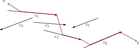
Figure 1: Illustrating a quickest path from a source point $s$ to a destination point $t$.

Problem 1

Given two points $s$ and $t$ in ${\mathbb{R}}^{2}$ and a transportation network ${\cal T}(S,{\cal C})$ in the Euclidean plane. The problem is to find a path with the smallest transportation distance from $s$ to $t$, as shown in Fig. 1.

Most of the previous research has focussed on shortest paths and Voroni diagrams. Abellanas et al. [1, 2] started work in this area considering the Voronoi diagram of a point set and shortest paths given a horizontal highway under the $L_{1}$-metric and the Euclidean metric. Aichholzer et al. [4] introduced the city metric induced by the $L_{1}$-metric and a highway network that consists of a number of axis-parallel line segments. They gave an efficient algorithm for constructing the Voronoi diagram and a quickest path map for a set of points given the city metric. Görke et al. [14] and Bae et al. [5] improved and generalised these results.

In the case when the edges can have arbitrary orientation and speed, Bae et al. [6] presented algorithms that compute the Voronoi diagram and shortest paths. They gave an algorithm for Problem 1 that uses $O(n^{3})$ time and $O(n^{2})$ space. This result was recently extended to more general metrics including asymmetric convex distance functions [7].

In this paper we improve on the results by Bae et al. [6] and give an $O(n^{2}\log n)$ time algorithm using $O(n^{2})$ space. Furthermore, we introduce the (approximate) query version. That is, a transportation network with $n$ roads in the Euclidean plane can be preprocessed in $O(n^{2}\log n)$ time into a data structure of size $O(n^{2}/\varepsilon^{2})$ such that given any two points $s$ and $t$ in the plane a $(1+\varepsilon)$-approximate quickest path between $s$ and $t$ can be answered in $O(1/\varepsilon^{4}\cdot\log n)$ time. For the query structure we assume that the minimum and maximum weights, $\alpha_{\min}$ and $\alpha_{\max}$, are constants in the interval $(0,1]$ independent of $n$, the exact bound is stated in Theorem 4.6.

This paper is organized as follows. Next we prove three fundamental properties about an optimal path among a set of roads. Then, in Section 3, we show how we can use these properties to build a graph of size $O(n^{2})$ that models the transportation network, a source point $s$, a destination point $t$ and, contains a quickest path between $s$ and $t$. In Section 4 we consider the query version of the problem. That is, preprocess the input such that an approximate quickest path query between two query points $s$ and $t$ can be answered efficiently. Finally, we conclude with some remarks and open problems.

2 Three Properties of an Optimal Path

In this section we are going to prove three important properties of an optimal path. The properties will be used repeatedly in the construction of the algorithms in Sections  3 and 4. Consider an optimal path ${\cal P}$ and let ${\cal C}_{{\cal P}}=\langle c_{1},c_{2},\ldots,c_{k}\rangle$ be the sequence of roads that are encountered and followed in order along ${\cal P}$, that is, the sequence of roads on which the path changes direction. For example, in Fig. 1 that sequence would be $\langle c_{1},c_{4},c_{6}\rangle$ but not include $c_{3}$ since the path does not follow $c_{3}$. For any path ${\cal P}_{1}$, let $wt({\cal P}_{1})$ denote the cost of the path ${\cal P}_{1}$. Note that a road can be encountered, and followed, several times by a path. For each road $c_{i}\in{\cal C}_{{\cal P}}$ let $s_{i}$ and $t_{i}$ be the first and last point on $c_{i}$ encountered for each occasion by ${\cal P}$. Without loss of generality, we assume that $t_{i+1}$ lies below $s_{i}$ when studying two consecutive roads in ${\cal C}_{{\cal P}}$. We have:

Property 1

For any two consecutive roads $c_{i}$ and $c_{i+1}$ in ${\cal C}_{{\cal P}}$ the subpath of ${\cal P}$ between $t_{i}$ and $s_{i+1}$ is the straight line segment $(t_{i},s_{i+1})$.

The endpoints of a road $c_{j}=(u_{j},v_{j})$ are denoted start point ($u_{j}$) and end point ($v_{j}$), as they appear along the road direction.

Consider a segment $(t_{i},s_{i+1})$ connecting two consecutive roads $c_{i}$ and $c_{i+1}$ along ${\cal C}_{{\cal P}}$. Let $\phi_{i+1}$ denote the angle $\angle(t_{i},s_{i+1},u_{i+1})$, as illustrated in Fig. 2(a).

Property 2

If $s_{i+1}$ lies in the interior of $c_{i+1}$ then $\phi_{i+1}=\arccos(\alpha_{i+1})$.

Proof

For simplicity rotate ${\cal C}$ such that $c_{i+1}$ is horizontal and lies below $t_{i}$, as shown in Fig. 2(a). Let $r$ denote the orthogonal projection of $t_{i}$ onto the ray containing $c_{i+1}$ (not necessarily on $c_{i+1}$ and let $h=|t_{i}r|$. We have:

$$|t_{i}s_{i+1}|=\frac{h}{\sin\phi_{i+1}}\quad{\rm and}\quad|rs_{i+1}|=h\cdot\frac{\cos\phi_{i+1}}{\sin\phi_{i+1}}.$$

Thus, the cost of the path from $t_{i}$ to $t_{i+1}$ along ${\cal C}_{{\cal P}}$ as a function of $\phi_{i+1}$ is:

$$f(\phi_{i+1})=|t_{i}s_{i+1}|+\alpha_{i+1}\cdot|s_{i+1}t_{i+1}|=\frac{h}{\sin\phi_{i+1}}+\alpha_{i+1}\cdot(|rt_{i+1}|-h\cdot\frac{\cos\phi_{i+1}}{\sin\phi_{i+1}}).$$

Differentiating the above function with respect to $\phi_{i+1}$ gives:

$$f^{\prime}(\phi_{i+1})=\frac{h(\cos\phi_{i+1}-\alpha_{i+1})}{\cos^{2}\phi_{i+1}-1}.$$

Setting $f^{\prime}(\phi_{i+1})=0$ the resulting function gives that the minimum weight path between $t_{i}$ and $t_{i+1}$ along ${\cal C}({\cal P})$ is obtained when

$$\phi_{i+1}=\arccos(\alpha_{i+1}).$$

$\square$

Property 3

There exists an optimal path ${\cal P}^{\prime}$ of total cost $wt({\cal P})$ with ${\cal C}_{{\cal P}^{\prime}}={\cal C}_{{\cal P}}$ that fulfills Properties 1-2 such that for any two consecutive roads $c_{i}$ and $c_{i+1}$ in ${\cal C}_{{\cal P}^{\prime}}$ the straight-line segment $(t_{i},s_{i+1})$ of ${\cal P}^{\prime}$ must have an endpoint at an endpoint of $c_{i}$ or $c_{i+1}$, respectively.

Proof

Assume the opposite, i.e., $(t_{i},s_{i+1})$ does not coincide with any of the endpoints of $c_{i}$ or $c_{i+1}$. Consider the three segment path from $s_{i}$ to $t_{i+1}$, that is, $(s_{i},t_{i})$, $(t_{i},s_{i+1})$ and $(s_{i+1},t_{i+1})$. The length of this path is:

$$\alpha_{i}\cdot|s_{i},t_{i}|+|t_{i},s_{i+1}|+\alpha_{i+1}\cdot|s_{i+1},t_{i+1}|.$$

According to Lemma 2 the orientation of $(t_{i},s_{i+1})$ is fixed, which implies that the weight of the path is a linear function only depending on the position of $t_{i}$ (or $s_{i+1}$). Hence, moving $t_{i}$ in one direction will monotonically increase the weight of the path until one of two cases occur: (1) either $t_{i}$ or $s_{i+1}$ encounters an endpoint of $c_{i}$ or $c_{i+1}$, or (2) $t_{i}=s_{i}$ or $s_{i+1}=t_{i+1}$. If (1) then we have a contradiction since we assumed $(t_{i},s_{i+1})$ did not coincide with any endpoint. And if (2) then we have a contradiction since ${\cal P}$ must follow both $c_{i}$ and $c_{i+1}$ (again from the definition of ${\cal C}_{{\cal P}}$). $\square$

Figure 2: (a) Illustrating Property 2. (b) Defining $PR_{f}(s,c_{i})$ and (c) $PR_{b}(t,c_{i})$.

3 The basic case

In this section we consider Problem 1, that is, as input we are given a source point $s$, a destination point $t$ and a transportation network ${\cal T}(S,{\cal C})$ and the aim is to find a path with minimum transportation distance from $s$ to $t$. Our algorithm will construct a graph $G$ that models the set ${\cal C}$ of roads and quickest paths between the roads. Using the three properties shown in the previous section we will show that if a shortest path in $G$ between $s$ and $t$ has cost $W$ then an optimal path between $s$ and $t$ has cost $W$. The optimal path can then be found by running Dijkstra’s algorithm [13] on $G$.

Fix an optimal path ${\cal P}$ that fulfills Properties 1-3 (we know such a path exists). If ${\cal P}$ follows $c_{i}$ and $c_{i+1}$ then the path between $c_{i}$ and $c_{i+1}$ (a) is a straight line segment, (b) the segment $(t_{i},s_{i+1})$ forms a fixed angle with $c_{i+1}$, and (c) at least one of its endpoints coincides with an endpoint of $c_{i}$ or $c_{i+1}$. These three properties suggest that ${\cal P}$ has a very restricted structure which we will try to take advantage of.

Let $PR_{f}(p,c_{i})$ be the projection of a point $p$ onto a road $c_{i}$, if it exists, such that the angle $\angle(p,PR_{f}(p,c_{i}),u_{i})$ is $\phi_{i}$, as shown in Fig. 2(b). Furthermore, let $PR_{b}(p,c_{i})$ be the projection of point $p$ on a road $c_{i}$, if it exists, such that the angle $\angle(p,PR_{b}(p,c_{i}),v_{i})$ is $\phi_{i}$, as shown in Fig. 2(c).

Consider the graph $G(V,E)$ with vertex set $V$ and edge set $E$. Initially $V$ and $E$ are empty. The graph $G$ is defined as follows:

1. Add $s$ and $t$ as vertices to $V$.

2. Add the nodes in $S$ as vertices to $V$.

3. For every road $c_{i}\in{\cal C}$ add the point $PR_{f}(s,c_{i})$ (if it exists) as a vertex to $V$ and add the directed edge $(s,PR_{f}(s,c_{i}))$ (if it exists) with weight $|sPR_{f}(s,c_{i})|$ to $E$, see Fig. 3(a).

4. For every road $c_{i}\in{\cal C}$ add the point $PR_{b}(t,c_{i})$ (if it exists) as a vertex to $V$ and add the directed edge $(PR_{b}(s,c_{i}),t)$ (if it exists) with weight $|PR_{b}(s,c_{i})t|$ to $E$.

5. For every pair of roads $c_{i},c_{j}\in{\cal C}$ add the following points (if they exist) as vertices to $V$: $PR_{f}(v_{i},c_{j})$, $PR_{f}(u_{i},c_{j})$, $PR_{f}(u_{j},c_{i})$ and $PR_{f}(v_{j},c_{i})$. Add the following four directed edges to $E$ (if their endpoints exist): $(v_{i},PR_{f}(v_{i},c_{j}))$, $(u_{i},PR_{f}(u_{i},c_{j}))$, $(v_{j},PR_{f}(v_{j},c_{i}))$ and $(u_{j},PR_{f}(u_{j},c_{i}))$. The weight of an edge is equal to the Euclidean distance between its endpoints, see Fig. 3(b).

6. For every pair of roads $c_{i},c_{j}\in{\cal C}$ add the directed edges $(v_{i},u_{j})$ with weight $|v_{i}u_{j}|$ and $(v_{j},u_{i})$ with weight $|v_{j}u_{i}|$ to $E$.

7. For every road $c_{i}$ consider the vertices of $V$ that correspond to points on $c_{i}$ in order from $u_{i}$ to $v_{i}$. For every consecutive pair of vertices $x_{j},x_{j+1}$ along $c_{i}$ add a directed edge from $x_{j}$ to $x_{j+1}$ of weight $\alpha_{i}\cdot|x_{j}x_{j+1}|$, as shown in Fig. 3(c).

Figure 3: Illustrating how the graph is built.

Lemma 1

The graph $G$ contains $O(n^{2})$ vertices and $O(n^{2})$ edges and can be constructed in time $O(n^{2}\log n)$.

Proof

For every pair of roads we construct a constant number of vertices and edges that are added to $V$ and $E$, thus $O(n^{2})$ vertices and edges in total. For the first five steps of the construction the time to construct the vertices and edges is linear with respect to the size of the graph, since every edge and vertex can be constructed in constant time. In step 6 we need to sort $O(n)$ vertices along each road, thus $O(n^{2}\log n)$ time in total. $\square$

The following observation follows immediately from the construction of the graph and Properties 1-3.

Observation 1

The shortest path between $s$ and $t$ in $G$ has cost $W$ if and only if the minimum transportation distance from $s$ to $t$ has cost $W$.

By simply running Dijkstra’s algorithm [13], implemented using Fibonacci heaps, on $G$ gives the main result of this section.

Theorem 3.1

A path with minimum transportation distance between $s$ and $t$ can be computed in $O(n^{2}\log n)$ time using $O(n^{2})$ space.

3.1 Shortest paths among polygon obstacles

In this section we briefly discuss how the above algorithm can be generalised to the case when the plane contains polygonal obstacles. As input we are given a source point $s$, a destination point $t$, a transportation network ${\cal T}(S,{\cal C})$ in the Euclidean plane and a set ${\cal O}$ of $k$ non-intersecting obstacles of total complexity $m$.

Every edge of an obstacle can be viewed as an undirected road (or two directed edges) with associated cost function $\alpha=1$. Consequently, the edge connecting a road and an obstacle edge along the optimal path has the three properties described in Section 2. However, while constructing the graph we have to add one additional constraint, namely, no edge in $E$ can intersect an obstacle. According to these properties we are going to build the graph $G$ that models the set of roads and obstacles.

There are several methods to check if a segment intersects an obstacle [3, 12, 15]. We will use the data structure by Agarwal and Sharir [3] which has $O(m^{1+\varepsilon}/\sqrt{L})$ query time using $O(L^{1+\varepsilon})$ preprocessing and space for $m\leq L\leq m^{2}$. Using this structure with $L=m^{2}$ gives us the following results:

Lemma 2

The graph $G$ has size $O(N^{2+\varepsilon})$ and can be constructed in time $O(N^{2+\varepsilon})$, where $N=n+m$.

By simply running Dijkstra’s algorithm, implemented using Fibonacci heaps, on $G$ gives:

Theorem 3.2

A collision-free path with minimum transportation distance between $s$ and $t$ among ${\cal O}$ can be computed in $O(N^{2}\log N)$ time using $O(N^{2})$ space, where $N=n+m$.

4 Shortest Path Queries

In this section we turn our attention to the query version. That is, preprocess ${\cal C}$ such that given any two points $s$ and $t$ in ${\mathbb{R}}^{2}$ find a quickest path between $s$ and $t$ among ${\cal C}$ effectively. We will present a data structure ${\cal D}$ that returns an approximate quickest path. That is, given two query points $s$ and $t$, and a positive real value $\varepsilon$, the data structure returns a path between $s$ and $t$ having transportation distance at most $(1+\varepsilon)$ times the cost of an optimal path between $s$ and $t$.

To simplify the description we will start (Sections 4.1-4.2) with the case when $t$ is already known in advance and we are only given the start point $s$ as a query. Then in Section 4.4 we generalize this to the case when both $s$ and $t$ are given as a query, and in Section 4.5 we show how one can improve the preprocessing time and space requirement using the well-separated pair decomposition.

Fix an optimal path ${\cal P}$ that fulfills Properties 1-3 (we know such a path exists), and consider the first segment $\ell=(s,s_{1})$ of ${\cal P}$. Obviously $s_{1}$ must be either a start/endpoint of a road (type 1) or an interior point of a road $c_{i}\in{\cal C}$ (type 2) such that $\ell$ and $c_{i}$ form an angle of $\phi_{i}$ (ignoring the trivial case when $s_{1}=t$). We will use this observation to develop an approximation algorithm. The idea is simple. Build a graph $G(V,E)$, as described in Section 3, with ${\cal T}$ and $t$ as input. Compute the cost of the quickest path between $t$ and every vertex in $V$. Now, given a query point $s$, find a good vertex $s_{1}$ in $V$ to connect $s$ (either directly or via a $2$-link path) to and then lookup the cost of the quickest path from $s_{1}$ to $t$ in $G$. Obviously the problem is how to find a “good” vertex. In the next subsection we will select a constant number of candidate vertices such that we can guarantee that at least one of the vertices will be a “good” candidate, i.e., there exists a path, that fulfills Properties 1-3, from $s$ to $t$ via this vertex that has cost at most $(1+\varepsilon)$ times the cost of an optimal path.

4.1 Finding good candidates: Type 1 and Type 2

Let ${\cal S}_{{\cal C}}$ denote the set of the endpoints (both start and end) of the roads in ${\cal C}$ and let $s$ be the query point. As described above we will have two types to consider, and we will construct a set ${\cal D}_{1}$ for the type 1 cases and a set ${\cal D}_{2}$ for the type 2 cases. The first set, ${\cal D}_{1}$, is a subset of ${\cal S}_{{\cal C}}$ and the second set, ${\cal D}_{2}$, is a set of 3-tuples that will be used by the query process (described in Section 4.2) to calculate the quickest path.

4.1.1 Type 1:

For the point set ${\cal D}_{1}$ we will use the same idea as is used in the construction of $\theta$-graphs [17]. Partition the plane into a set of $k=\max\{9,\frac{36\pi}{\varepsilon}\}$ equal size cones, denoted $X_{1},\ldots,X_{k}$, with apex at $s$ and spanning an angle of $\theta=2\pi/k$, as shown in Fig. 4a. For each cone $X$ the set ${\cal D}_{1}$ contains a point $r$, where $r$ is a point in ${\cal S}_{{\cal C}}\cap X$ whose orthogonal projection onto the bisector of $X$ is closest to $s$. The following holds:

Lemma 3

Given a point set ${\cal S}_{{\cal C}}$ and a positive constant $\varepsilon$ one can preprocess ${\cal S}_{{\cal C}}$ into a data structure of size $O(n/\varepsilon)$ in $O(1/\varepsilon\cdot n\log n)$ time such that given a query point $s$ the point set ${\cal D}_{1}$, of size at most $36\pi/\varepsilon$, can be reported in $O(1/\varepsilon\cdot\log n)$ time.

Proof

Given a direction $d$ and a point $s$ let $\ell_{d}(s)$ denote the infinite ray originating at $s$ with direction $d$, see Fig. 4b. Let $C(s,d,\theta)$ be the cone with apex at $s$, bisector $\ell_{d}(s)$ and angle $\theta$. It has been shown (see for example Section 4.1.2 in [17] or Lemma 2 in [10]) that ${\cal S}_{{\cal C}}$ can be preprocessed in $O(n\log n)$ time into a data structure of size $O(n)$ such that given a query point $s$ in the plane the data structure returns the point in $C(s,d,\theta)$ whose orthogonal projection onto $\ell_{d}(s)$ is closest to $s$ in $O(\log n)$ time. We have $36\pi/\varepsilon$ directions, thus the lemma follows. $\square$

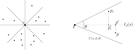
Figure 4: (a) Partitioning the plane into $k$ cones. (b) Selecting the point whose orthogonal projection onto the bisector of $X$.

4.1.2 Type 2:

It remains to construct the set ${\cal D}_{2}$ of $3$-tuples. Unfortunately the construction might look unnecessarily complicated but hopefully it will become clear, when we prove the approximation bound (Section 4.3) why we need this construction. Before constructing ${\cal D}_{2}$ we need some basic definitions.

Let $\alpha_{\max}$ and $\alpha_{\min}$ be the maximum and minimum weight of the roads in ${\cal C}$. Partition the set ${\cal C}$ of roads into a minimum number of sets, ${\cal C}_{1},\ldots,{\cal C}_{m}$, such that the orientation of a road in ${\cal C}_{i}$ is in $[(i-1)\theta\cdot\alpha_{\min},i\theta\cdot\alpha_{\min})$, where $\theta=\varepsilon/18$. Partition each set ${\cal C}_{i}$, $1\leq i\leq m$, into $b$ sets ${\cal C}_{i,1},\ldots,{\cal C}_{i,b}$ such that the weight of a road in ${\cal C}_{i,j}$ is in $[\alpha_{\min}\cdot(1+\varepsilon)^{j-1},\alpha_{\min}\cdot(1+\varepsilon)^{j})$.

For every $i,j$, $1\leq i\leq m$ and $1\leq j\leq b$, define two directions $\gamma_{up}(i,j)$ and $\gamma_{down}(i,j)$ as follows (see also Fig. 5a). Consider an infinite ray $\Upsilon$ with orientation $(i-1)\theta$ having weight $\alpha=\alpha_{\min}\cdot\varepsilon^{j-1}$. For simplicity we rotate the ray such that it is horizontal directed from left to right. Let $\gamma_{up}(i,j)$ be the direction of a ray $r$ originating from below $\Upsilon$ such that $r$ and $\Upsilon$ meet at an angle of $\arccos(\alpha)$. The direction $\gamma_{down}(i,j)$ is defined symmetrically but with a ray originating from above $\Upsilon$.

Given a point $p$ on a road $c$ let $N(p,c)$ denote the nearest vertex of $G$ to $p$ along $c$. Note that $N(p,c)$ must lie between $p$ and the end point of $c$.

Now, we are ready to construct ${\cal D}_{2}$. When given the query point $s$ construct the set ${\cal D}_{2}$ as follows. For each $i,j$, $1\leq i\leq m$ and $1\leq j\leq b$, shoot a ray $r_{up}$ originating from $s$ in direction $\gamma_{up}(i,j)$ and one ray $r_{down}$ in direction $\gamma_{down}(i,j)$. If $r_{up}$ hits a road in ${\cal C}_{i,j}$ then let $c_{up}$ be the first road hit and let $p_{up}$ be the point hit on $c_{up}$, as illustrated in Fig. 5b. The $3$-tuple $[c_{up},p_{up},N(p_{up},c_{up})]$ is added to ${\cal D}_{2}$. If $r_{down}$ hits a road in ${\cal C}_{i,j}$ then let $c_{down}$ be the first road hit and let $p_{down}$ be the point hit on $c_{down}$. The $3$-tuple $[c_{down},p_{down},N(p_{down},c_{down})]$ is added to ${\cal D}_{2}$.

Lemma 4

Given a transportation network ${\cal T}(S,{\cal C})$ with $n$ roads in the Euclidean plane and a positive constant $\varepsilon$ one can preprocess ${\cal T}$ in $O(n\log n)$ time into a data structure of size $O(n)$ such that given a query point $s$ the set ${\cal D}_{2}$ can be reported in $O(\frac{1}{\alpha_{\min}\cdot\varepsilon^{2}}\cdot\log n\log_{1+\varepsilon}\frac{\alpha_{\max}}{\alpha_{\min}})$ time. The number of $3$-tuples in ${\cal D}_{2}$ is $O(\frac{1}{\alpha_{\min}\varepsilon^{2}}\cdot\log_{1+\varepsilon}\frac{\alpha_{\max}}{\alpha_{\min}})$.

Proof

The preprocessing consists of two steps: (1) partitioning ${\cal C}$ into the sets ${\cal C}_{i,j}$, $1\leq i\leq m$ and $1\leq j\leq b$, and (2) preprocessing each set ${\cal C}_{i,j}$ into a data structure that answers ray shooting queries efficiently.

The first part is easily done in $O(n\log n)$ time by sorting the roads first with respect to their orientation and then with respect to their weight.

The second step of the preprocessing can be done by building two trapezoidal maps $T_{up}({\cal C}_{i,j})$ and $T_{down}({\cal C}_{i,j})$ (also know as a vertical decomposition) of each set ${\cal C}_{i,j}$ as follows (see Fig. 5c). Rotate ${\cal C}_{i,j}$ such that $\gamma_{up}(i,j)$ is vertical and upward. Build a trapezoidal map $T_{up}({\cal C}_{i,j})$ of ${\cal C}_{i,j}$ as described in Chapter 6.1 in [8]. Then preprocess $T_{up}({\cal C}_{i,j})$ to allow for planar point location. Note that every face in $T({\cal C})$ either is a triangle or a trapezoid, and the left and right edges of each face (if they exists) are vertical. The trapezoidal map $T_{down}({\cal C}_{i,j})$ can be computed in the same way by rotating ${\cal C}_{i,j}$ such that $\gamma_{down}(i,j)$ is vertical and upward. The total time needed for this step is $O(n\log n)$ and it requires $O(n)$ space.

When a query point $s$ is given, two ray shooting queries are performed for each set ${\cal C}_{i,j}$. However, instead we perform a point location in the trapezoidal maps $T_{up}({\cal C}_{i,j})$ and $T_{down}({\cal C}_{i,j})$. Consider $T_{up}({\cal C}_{i,j})$ and let $f$ be the face in the map containing $s$. The top edge of $f$ corresponds to the first road $c_{up}$ hit by a ray emanating from $s$ in direction $\gamma_{up}(i,j)$. When $c_{up}$ is found we just add to ${\cal D}_{2}$ the first vertex on $c_{up}$ in $G$ to the right of $s$. The same process is repeated for $T_{down}({\cal C}_{i,j})$. Performing the point location requires $O(\log n)$ time per trapezoidal map, thus the total query time is $O(mb\log n)=O(\frac{1}{\alpha_{\min}\cdot\varepsilon^{2}}\cdot\log n\log_{1+\varepsilon}(\alpha_{\max}/\alpha_{\min}))$. $\square$

Figure 5: (a) Illustrating the definition of $\gamma_{up}(i,j)$ and $\gamma_{down}(i,j)$. (b) $p_{up}$ is the first point hit by the ray and $N(c_{up},p_{up})$ is the nearest neighbour of $p_{up}$ along $c_{up}$. (c) The trapezoidal map of a set ${\cal C}_{i,j}$ and the query point $s$.

4.2 The preprocessing and the query

In this section we will present the remaining data structure, define the preprocessing and show how a query is processed.

4.2.1 Preprocessing

In Section 3 we showed how to build a graph given two points and the transportation network ${\cal T}(S,{\cal C})$. The first step of the preprocessing is to build a graph $G(V,E)$ of ${\cal C}$ and the destination point $t$ (without the source point). Next compute the shortest path from every vertex in $G$ to the vertex corresponding to $t$. Since the complexity of $G$ is quadratic, this step can be done in $O(n^{2}\log n)$ time and $O(n^{2})$ space using Dijkstra’s algorithm. The distances are saved in a matrix $M$. Finally, we combine the above results with Lemmas 3 and 4 and get:

Theorem 4.1

The preprocessing requires $O(n^{2}\log n)$ time and $O(n^{2})$ space.

4.2.2 Query

As a query we are given a point $s$ in the plane. First we compute the two sets ${\cal D}_{1}$ and ${\cal D}_{2}$. For each vertex $s_{1}$ in ${\cal D}_{1}$ compute the quickest path via $s_{1}$, that is, $|ss_{1}|+M[s_{1},t]$. The quickest among these paths is denoted ${\cal P}_{1}$. The $3$-tuples in ${\cal D}_{2}$ require slightly more computation. For each $3$-tuple $[c,s_{1},s_{2}]$ consider the path from $s$ to $t$ using $(s,s_{1})$ and $(s_{1},s_{2})$. The cost of the path can be calculated as $|ss_{1}|+\alpha\cdot|s_{1}s_{2}|+M[s_{2},t]$, where $\alpha$ is the weight of road $c$. The quickest among these paths is denoted ${\cal P}_{2}$.

The quickest path among ${\cal P}_{1}$, ${\cal P}_{2}$ and the direct path from $s$ to $t$ is then reported.

Theorem 4.2

A query can be answered in time $O(\frac{1}{\alpha_{\min}\varepsilon^{2}}\cdot\log n\log_{1+\varepsilon}\frac{\alpha_{\max}}{\alpha_{\min}})$.

Proof

As above we divide the analysis into two parts: type 1 and type 2.

Type 1: According to Lemma 3 the number of type 1 candidate points is at most $32\pi/\varepsilon$ and can be computed in time $O(1/\varepsilon\cdot\log n)$. Computing the cost of a quickest path for a point in ${\cal D}_{1}$ can be done in constant time. Thus, the query time is $O(1/\varepsilon\log n)$.

Type 2: According to Lemma 4 the number of $3$-tuples in ${\cal D}_{2}$ is $O(\frac{1}{\alpha_{\min}\varepsilon^{2}}\cdot\log_{1+\varepsilon}\alpha_{\max}/\alpha_{\min})$ and can be computed in time $O(\frac{1}{\alpha_{\min}\varepsilon^{2}}\cdot\log n\log_{1+\varepsilon}\alpha_{\max}/\alpha_{\min})$. Each element in ${\cal D}_{2}$ is then processed in $O(1)$ time, thus $O(\frac{1}{\alpha_{\min}\varepsilon^{2}}\cdot\log n\log_{1+\varepsilon}\alpha_{\max}/\alpha_{\min})$ in total.

Summing up we get the bound stated in the theorem. $\square$

4.3 Approximation bound

Consider an optimal path ${\cal P}$ and let $\ell=(s,s_{1})$ be the first segment of ${\cal P}$. According to Property 1 it is a straight-line segment. For any two points $p_{1}$ and $p_{2}$ along ${\cal P}$, let $\delta_{G}(p_{1},p_{2})$ denote the cost of ${\cal P}$ from $p_{1}$ to $p_{2}$. Define $s(\ell)$ to be the sector with apex at $s$, bisector on $\ell$, interior angle $\kappa=\varepsilon/18$ and radius $(1+4\kappa)\cdot|ss_{1}|$, as shown in Fig. 6(a).

Lemma 5

Let $\varepsilon$ be a positive constant. If $s(\ell)\cap{\cal S}_{{\cal C}}\neq\emptyset$ then:

$$wt({\cal P})\leq wt({\cal P}_{1})\leq(1+\varepsilon)\cdot wt({\cal P}).$$

Proof

The proof will be shown in two steps: (1) first we prove that for every endpoint $p$ within $s(\ell)$ the quickest path, denoted ${\cal P}(p)$, from $s$ to $t$ using the segment $(s,p)$ has cost at most $(1+12\kappa)\cdot wt({\cal P})$, and then (2) we prove that $wt({\cal P}_{1})$ has cost at most $(1+3\kappa)\cdot wt({\cal P}(p))$. Combining the two parts proves the lemma.

Part 1: Consider any point $p$ within $s(\ell)$, and let ${\cal P}(p)$ denote the quickest path from $s$ to $t$ using the segment $(s,p)$. We have:

$$wt({\cal P}(p)) = |sp|+\delta_{G}(p,t)$$

$$\leq |sp|+|ps_{1}|+\delta_{G}(s_{1},t)$$

$$\leq (1+4\kappa)\cdot|ss_{1}|+\sqrt{(\cos\frac{\kappa}{2}-1-4\kappa)^{2}+\sin^{2}\frac{\kappa}{2}}\cdot|ss_{1}|+\delta_{G}(s_{1},t)$$

$$< (1+12\kappa)\cdot|ss_{1}|+\delta_{G}(s_{1},t)$$

$$\leq (1+12\kappa)\cdot\delta_{G}(s,t)$$

Part 2: As above let $p$ be any endpoint of ${\cal C}$ within $s(\ell)$, and let ${\cal P}(p)$ be the quickest path from $s$ to $t$ using the segment $|sp|$.

Consider the set ${\cal D}_{1}$ as described in Section 4.1 and assume without loss of generality that $p$ lies in a cone $X$. If there exists a point $q$ in ${\cal D}_{1}$ such that $q=p$ then we are done since $|sq|+\delta_{G}(q,t)=wt({\cal P}(p))$.

Otherwise, there must exist another point $q$ in ${\cal D}_{1}$ such that $q\in X$ and whose orthogonal projection $q^{\prime}$ onto the bisector of $X$ is closer to $s$ than the orthogonal projection $p^{\prime}$ of $p$ onto the bisector of $X$.

$$wt({\cal P}(q)) \leq |sq|+|qp|+\delta_{G}(p,t)$$

$$\leq |sq|+|qq^{\prime}|+|q^{\prime}p^{\prime}|+|p^{\prime}p|+\delta_{G}(p,t)$$

$$\leq |sq^{\prime}|(\frac{1}{\cos\kappa}+\frac{\sin\kappa}{\cos\kappa})+|q^{\prime}p^{\prime}|+|sp|\cdot\sin\kappa+\delta_{G}(p,t)$$

$$< (|sq^{\prime}|+|q^{\prime}p^{\prime}|)(\frac{1}{\cos\kappa}+\frac{\sin\kappa}{\cos\kappa})+|sp|\cdot\sin\kappa+\delta_{G}(p,t)$$

$$\leq |sp|(\frac{1}{\cos\kappa}+\frac{\sin\kappa}{\cos\kappa}+\sin\kappa)+\delta_{G}(p,t)$$

$$< \frac{|sp|}{\cos\kappa}(1+2\sin\kappa)+\delta_{G}(p,t)$$

$$< |sp|\cdot(1+3\cot\kappa)+\delta_{G}(p,t)$$

$$< (1+3\kappa)\cdot wt({\cal P}(p))$$

In the last step we used that $\kappa=\varepsilon/18<2\pi/9$.

Now we can combine the two results as follows.

$$wt({\cal P}_{1}) \leq wt({\cal P}(q))$$

$$\leq (1+12\kappa)\cdot\delta_{G}(p,t)\hskip 75.39963pt\mathrm{(from~{}Part~{}1)}$$

$$\leq (1+3\kappa)\cdot(1+12\kappa)\cdot\delta_{G}(s,t)\hskip 28.45274pt\mathrm{(from~{}Part~{}2)}$$

$$< (1+\varepsilon)\cdot\delta_{G}(s,t)\hskip 88.2037pt\mathrm{(since~{}}\kappa=\varepsilon/18\mathrm{~{}and~{}}\varepsilon<1)$$

This completes the proof of the lemma. $\square$

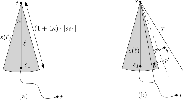
Figure 6: (a) Illustrating the definition of $s(\ell)$. (b) Illustrating the setting in Lemma 6.

Lemma 6

Let $\varepsilon<1$ be positive constants. If $s(\ell)\cap{\cal S}_{{\cal C}}=\emptyset$ then:

$$wt({\cal P})\leq wt({\cal P}_{2})\leq(1+\varepsilon)\cdot wt({\cal P}).$$

Proof

As above let $(s,s_{1})$ be the first segment of ${\cal P}$, where $s_{1}$ lies on a road $c_{1}$. Assume w.l.o.g. that $c_{1}$ is belongs to the set of roads ${\cal C}_{ij}$ as defined in Section 4.1(Type 2). Rotate the input such that $c_{1}$ is horizontal, below $s$ and going from right to left. Consider the construction of the $3$-tuples in Type 2, and let $[c^{\prime}_{1},s^{\prime}_{1},p]$ be the $3$-tuple reported when ${\cal C}_{ij}$ was processed in the direction towards $c_{1}$. See Fig. 7(b).

Consider the shortest path from $s$ to $t$ using the segment $(s,s^{\prime}_{1})$. We will have two cases depending on $s^{\prime}_{1}$: either (1) $s_{1}$ and $s^{\prime}_{1}$ lie on the same road, or (2) they lie on different roads.

Case 1: If $s^{\prime}_{1}$ and $s_{1}$ both lie on road $c_{1}$ (with cost function $\alpha_{1}$) then we have:

$$wt({\cal P}_{2}) \leq |ss^{\prime}_{1}|+\alpha_{1}\cdot|s^{\prime}_{1},t_{1}|+\delta_{G}(t_{1},t)$$

$$\leq |ss^{\prime}_{1}|+\alpha_{1}\cdot|s^{\prime}_{1}s_{1}|+\alpha_{1}\cdot|s_{1}t_{1}|+\delta_{G}(t_{1},t)$$

$$\leq |ss^{\prime}_{1}|+\alpha_{1}\cdot|s^{\prime}_{1}s_{1}|+\delta_{G}(s_{1},t)$$

$$\leq (1+4\kappa)\cdot|ss_{1}|+5\kappa\cdot|ss_{1}|+\delta_{G}(s_{1},t)\quad\mathrm{(since~{}}\theta\leq\kappa)$$

$$\leq (1+9\kappa)\cdot|ss_{1}|+\delta_{G}(s_{1},t)$$

$$\leq (1+9\kappa)\cdot\delta_{G}(s,t)$$

$$< (1+\varepsilon)\cdot\delta_{G}(s,t)$$

That completes the first part.

Part 2: If $s^{\prime}_{1}$ and $s_{1}$ lie on different roads $c^{\prime}_{1}$ and $c_{1}$, respectively, then $c^{\prime}_{1}$ must lie between $s$ and $c_{1}$. This follows from the fact that $s(\ell)$ does not contain any endpoints and $c^{\prime}_{1}$ is the first road hit. Furthermore, there must exist a an edge $(q^{\prime},q)\in E$ such that $q^{\prime}$ lies on $c^{\prime}_{1}$ to the left of $s^{\prime}_{1}$ and $q$ lies on $c_{1}$ to the right of $t_{1}$ and $\angle(u_{1},q,q^{\prime})=\arccos\alpha_{1}$. See Fig. 7(b) for an illustration of case 2(a).

Consider the situation as depicted in Fig. 7(b). We will prove that the cost of the path from $s$ to $t_{1}$ via $s^{\prime}_{1},q^{\prime}$ and $q$ is almost the same as the cost of the optimal path from $s$ to $t_{1}$ (that goes via $s_{1})$. Recall that the cost function of $c_{1}$ and is $\alpha_{1}$ and the cost function of $c^{\prime}_{1}$ is $\alpha^{\prime}_{1}$. Furthermore, let $r$ be the intersection point between $c^{\prime}_{1}$ and $(s,s_{1})$.

Note that the cost of the path from $r$ to $q$ via $q^{\prime}$ is maximized if $rq^{\prime}$ forms an angle of $\theta$ with the horizontal line and $q^{\prime}$ lies above $r$, as shown in Fig. 7(b). Furthermore, $|qq^{\prime}|=|q^{\prime}p|+|pq|$ and $|pq|=|rs_{1}|$.

$$\alpha^{\prime}_{1}\cdot|rq^{\prime}|+|q^{\prime}p| \leq \alpha^{\prime}_{1}\cdot|pr|\cdot\cos\theta+|pr|\cdot\sin\theta$$

$$< |pr|(\alpha^{\prime}_{1}+\varepsilon\cdot\alpha_{\min}/18)$$

$$< \alpha^{\prime}_{1}\cdot|pr|(1+\varepsilon)$$

Putting together the bounds we get:

$$wt({\cal P}_{2}) \leq |ss^{\prime}_{1}|+\alpha^{\prime}_{1}\cdot|s^{\prime}_{1}q^{\prime}|+|q^{\prime}q|+\delta_{G}(q,t)$$

$$\leq |ss^{\prime}_{1}|+\alpha^{\prime}_{1}\cdot|s^{\prime}_{1}r|+\alpha^{\prime}_{1}\cdot|rq^{\prime}|+(|q^{\prime}p|+|pq|)+\delta_{G}(q,t)$$

$$\leq (1+9\kappa)\cdot|sr|+\alpha^{\prime}_{1}\cdot|rq^{\prime}|+|q^{\prime}p|+|rs_{1}|+\delta_{G}(q,t)\quad\mathrm{(see~{}Part~{}1)}$$

$$\leq (1+9\kappa)\cdot|sr|+|rs_{1}|+\alpha^{\prime}_{1}\cdot|pr|(1+\varepsilon)+\delta_{G}(q,t)$$

$$< (1+\varepsilon)\cdot(|sr|+|rs_{1}|+\alpha^{\prime}_{1}\cdot|s_{1}q|)+\delta_{G}(q,t)$$

$$< (1+\varepsilon)\cdot wt({\cal P})$$

This completes the proof of Lemma 6. $\square$

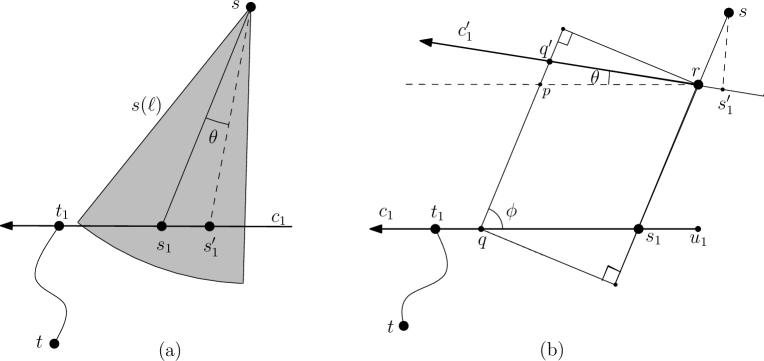
Figure 7: Illustrating (a) Case 1 and Case 2 (b) in the proof of Lemma 6.

We can summarize this section (Lemmas  5 and  6, Theorems  4.1 and  4.2) with the following theorem:

Theorem 4.3

Given a transportation network ${\cal T}$ with $n$ roads in the Euclidean plane, a destination point $t$ and a positive constant $\varepsilon$, one can preprocess ${\cal T}$ and $t$ in $O(n^{2}\log n)$ time and $O(n^{2})$ space such that given a query point $s$, a $(1+\varepsilon)$-approximate quickest path can be calculated in $O(\frac{1}{\alpha_{\min}\varepsilon^{2}}\cdot\log n\log_{1+\varepsilon}\frac{\alpha_{\max}}{\alpha_{\min}})$ time.

4.4 General case

In this section we turn our attention to the query version when we are given two query points $s$ and $t$ in ${\mathbb{R}}^{2}$ and our goal is to find a quickest path between $s$ and $t$ among ${\cal C}$. The idea is the same as in the previous section. That is we perform the exact same preprocessing steps as in the previous section (omitting the destination point $t$), but with the exception that $M$ contains all-pair shortest distances. Using Johnson’s algorithm [16] the all-pairs shortest paths can be computed in $O(n^{4}\log n)$ using $O(n^{4})$ space.

Given a query we compute the two candidate sets of type 1 and type 2 for both $s$ and $t$. For each pair of elements $p\in{\cal D}_{1}(s)\cup{\cal D}_{2}(s)$ and $q\in{\cal D}_{1}(t)\cup{\cal D}_{2}(t)$ compute a path between $s$ and $t$ as follows:

if $p\in{\cal D}_{1}$ and $q\in{\cal D}_{1}$ then $|sp|+M[p,q]+|qt|$

if $p\in{\cal D}_{1}$ and $q=[c,s_{1},s_{2}]\in{\cal D}_{2}$ then $|sp|+M[p,s_{2}]+\alpha(c)\cdot|s_{2}s_{1}|+|s_{1}s|$

if $p=[c,s_{1},s_{2}]\in{\cal D}_{2}$ and $q\in{\cal D}_{1}$ then $|ss_{1}|+\alpha(c)\cdot|s_{1}s_{2}|+M[s_{2},q]+|qt|$

if $p=[c_{1},s_{1},s_{2}]\in{\cal D}_{2}$ and $q=[c_{2},t_{1},t_{2}]\in{\cal D}_{2}$ then $|ss_{1}|+\alpha(c_{1})\cdot|s_{1}s_{2}|+M[s_{2},t_{2}]+\alpha(c_{2})\cdot|t_{2}t_{1}|+|t_{1}t|$

Note that for a specific pair $p,q$ the calculated distance might not be a good approximation of the actual distance. However, for the shortest path there exists a pair $p,q$ such that the distance is a good approximation.

By putting together the results, we obtain the following theorem:

Theorem 4.4

Given a transportation network ${\cal T}$ with $n$ roads in the Euclidean plane and a positive constant $\varepsilon$, one can preprocess ${\cal T}$ in $O(n^{4}\log n)$ time using $O(n^{4})$ space such that given two query points $s$ and $t$ a $(1+\varepsilon)$-approximate quickest path between $s$ and $t$ can be calculated in $O((\frac{1}{\alpha_{\min}\cdot\varepsilon^{2}}\cdot\log_{1+\varepsilon}\frac{\alpha_{\max}}{\alpha_{\min}})^{2}\cdot\log n)$ time.

4.5 Improving the complexity using the well-separated pair decomposition

The bottleneck of the preprocessing algorithm is the fact that $n^{4}$ shortest paths are computed in a graph of quadratic complexity. Is there a way to get around this? Since it suffices to approximate the shortest paths we can reduce the number of shortest path queries from $O(n^{4})$ to $O(n^{2})$, that is, linear in the number of vertices, using the well-separated pair-decomposition (WSPD).

Definition 1 ([11])

Let $s>0$ be a real number, and let $A$ and $B$ be two finite sets of points in ${\mathbb{R}}^{d}$. We say that $A$ and $B$ are well-separated with respect to $s$, if there are two disjoint $d$-dimensional balls $C_{A}$ and $C_{B}$, having the same radius, such that (i) $C_{A}$ contains the bounding box $R(A)$ of $A$, (i) $C_{B}$ contains the bounding box $R(B)$ of $B$, and (ii) the minimum distance between $C_{A}$ and $C_{B}$ is at least $s$ times the radius of $C_{A}$.

The parameter $s$ will be referred to as the separation constant. The next lemma follows easily from Definition 1.

Lemma 7 ([11])

Let $A$ and $B$ be two finite sets of points that are well-separated w.r.t. $s$, let $x$ and $p$ be points of $A$, and let $y$ and $q$ be points of $B$. Then (i) $|xy|\leq(1+4/s)\cdot|pq|$, and (ii) $|px|\leq(2/s)\cdot|pq|$.

Definition 2 ([11])

Let $S$ be a set of $n$ points in ${\mathbb{R}}^{d}$, and let $s>0$ be a real number. A well-separated pair decomposition (WSPD) for $S$ with respect to $s$ is a sequence of pairs of non-empty subsets of $S$, $(A_{1},B_{1}),\ldots,(A_{m},B_{m})$, such that

1. $A_{i}\cap B_{i}=\emptyset$, for all $i=1,\ldots,m$,

2. for any two distinct points $p$ and $q$ of $S$, there is exactly one pair $(A_{i},B_{i})$ in the sequence, such that (i) $p\in A_{i}$ and $q\in B_{i}$, or (ii) $q\in A_{i}$ and $p\in B_{i}$,

3. $A_{i}$ and $B_{i}$ are well-separated w.r.t. $s$, for $1\leq i\leq m$.

The integer $m$ is called the size of the WSPD.

Callahan and Kosaraju showed that a WSPD of size $m={\cal O}(s^{d}n)$ can be computed in ${\cal O}(s^{d}n+n\log n)$ time.

Construct the graph $G(V,E)$ of ${\cal T}$, as defined in Section 3. Compute a WSPD $\{(A_{i},B_{i})\}_{i=1}^{k}$ of $V$ with respect to a separation constant $s=\frac{8}{\tau\cdot\alpha_{\min}}$, where $\tau<1$ is a positive constant given as input. Then for each well-separated pair $(A_{i},B_{i})$ pick two arbitrary points $a\in A_{i}$ and $b\in B_{i}$ as representative points, and calculate the shortest path in $G$ between $a$ and $b$. All paths are stored in a matrix $M^{\prime}$. According to Definition 2, we have $O(n^{2})$ well separated pairs. It follows that the number of the shortest path queries in $M$ is $O(n^{2})$.

The queries are performed in almost the same way as above. The only difference is how the cost of the path between two points is calculated. Assume that we want the minimum transportation distance between two query points $p$ and $q$. According to Definition 2 there exists a well-separated pair $\{A,B\}$ such that $p\in A$ and $q\in B$, or vice versa. Furthermore, let $r_{A}$ and $r_{B}$ be the representative points of $A$ and $B$, respectively. Instead of using the value in $M[p,q]$ we approximate the cost by $|pr_{A}|+M^{\prime}[r_{A},r_{B}]+|r_{B}q|$.

Theorem 4.5

$$\delta_{G}(p,q)\leq|pr_{A}|+M^{\prime}[r_{A},r_{B}]+|r_{B}q|\leq(1+\tau)\cdot\delta_{G}(p,q).$$

Proof

The left inequality is immediate, thus we will focus on the right inequality.

$$|pr_{A}|+M^{\prime}[r_{A},r_{B}]+|r_{B}q| = |pr_{A}|+\delta_{G}(r_{A},r_{B})+|r_{B}q|$$

$$\leq 2|pr_{A}|+2|r_{B}q|+\delta_{G}(p,q)$$

$$\leq 4\cdot 2/s\cdot|pq|+\delta_{G}(p,q)$$

$$\leq \tau\cdot\alpha_{\min}\cdot|pq|+\delta_{G}(p,q)$$

$$\leq (1+\tau)\cdot\delta_{G}(p,q)$$

Where the last step follows by using $|pq|\leq\delta_{G}(p,q)/\alpha_{\min}$. $\square$

Given a positive constant $\sigma<1$ we can obtain the claimed bounds by setting the constants appropriately (for example $\tau=\sigma/3$ and $\varepsilon=\sigma/3)$. We get:

Theorem 4.6

Given a transportation network ${\cal T}(S,{\cal C})$ with $n$ roads and a positive constant $\varepsilon$, one can preprocess ${\cal C}$ in $O((\frac{n}{\alpha_{\min}\cdot\varepsilon})^{2}\log n)$ time using $O((\frac{n}{\alpha_{\min}\cdot\varepsilon})^{2})$ space such that given two query points $s$ and $t$ a $(1+\varepsilon)$-approximate quickest path between $s$ and $t$ can be calculated in $O((\frac{1}{\alpha_{\min}\cdot\varepsilon^{2}}\cdot\log_{1+\varepsilon}\frac{\alpha_{\max}}{\alpha_{\min}})^{2}\cdot\log n)$ time.

Assuming $\alpha_{\min}$ and $\alpha_{\max}$ being constants the bounds can be rewritten as: preprocessing is $O(n^{2}\log n)$, space is $O(n^{2}/\varepsilon^{2})$ and the query time is $O(1/\varepsilon^{4}\cdot\log n)$.

5 Concluding Remarks

We considered the problem of computing a quickest path in a transportation network. In the static case our algorithm has a running time of $O(n^{2}\log n)$ which is a linear factor better than the best algorithm known so far. We also introduce the query version of the problem.

There are many open problems remaining. For example, can one develop a more efficient data structure that has a smaller dependency on $\alpha_{\min}$ and $\varepsilon$? Also, is there a subquadratic time algorithm for the static case? If not, can we prove that the problem is 3sum-hard? Bae and Chwa [6] proved that the shortest path map for a transportation metric can have $\Omega(n^{2})$ size, which indicates that the problem may indeed be 3sum-hard.

References

- [1] M. Abellanas, F. Hurtado, C. Icking, R. Klein, E. Langetepe, L. Ma, B. Palop del Río and V. Sácristan. Proximity problems for time metrics induced by the L1 metric and isothetic networks. In Actas de los IX Encuentros de Geometr a Computacional, pages 175 182, Girona, 2001.
- [2] M. Abellanas, F. Hurtado, C. Icking, R. Klein, E. Langetepe, L. Ma, B. Palop del Río and V. Sácristan. Voronoi diagram for services neighboring a highway. Information Processessing Letters, 86:283 -288, 2003.
- [3] P. K. Agarwal and M. Sharir. Applications of a new space partitioning technique. Discrete & Computational Geometry, 9:11–38, 1993.
- [4] O. Aichholzer, F. Aurenhammer and B. Palop del Río. Quickest paths, straight skeletons, and the city Voronoi diagram. Discrete & Computatational Geometry, 31:17 -35, 2004.
- [5] S. W. Bae, J.-H. Kim and K.-Y. Chwa. Optimal construction of the city Voronoi diagram. International Journal on Computational Geometry & Applications, 19(2):95–117, 2009.
- [6] S. W. Bae and K.-Y. Chwa. Voronoi Diagrams for a Transportation Network on the Euclidean Plane. International Journal on Computational Geometry & Applications, 16:117–144, 2006.
- [7] S. W. Bae and K.-Y. Chwa. Shortest Paths and Voronoi Diagrams with Transportation Networks Under General Distances. ISAAC, pages 1007–1018, 2005.
- [8] M. de Berg, O. Cheong, M. van Kreveld and M. Overmars. Computational Geometry: Algorithms and Applications. (3rd edition). Springer-Verlag, Heidelberg, 2008.
- [9] J. L. Bentley. Multidimensional divide-and-conquer. Communications of the ACM, 23(5):214–228, 1978.
- [10] P. Bose, J. Gudmundsson and P. Morin. Ordered theta graphs. Computational geometry – Theory & Applications, 28(1):11–18, 2004.
- [11] P. B. Callahan and S. R. Kosaraju. A decomposition of multidimensional point sets with applications to -nearest-neighbors and -body potential fields. Journal of the ACM, 42:67–90, 1995.
- [12] S. W. Cheng and R. Janardan. Algorithms for ray-shooting and intersection searching. Journal of Algorithms 13:670–692, 1992.
- [13] E. W. Dijkstra. A note on two problems in connexion with graphs. Numerische Mathematik, 1:269 -271, 1959.
- [14] R. Görke, C.-C. Shin and A. Wolff. Constructing the City Voronoi Diagram Faster. International Journal of Computational Geometry and Applications 18(4):275–294, 2008.
- [15] J. Hershberger and S. Suri. A pedestrian approach to ray shooting: Shoot a ray, take a walk. Journal of Algorithms 18:403–431, 1995.
- [16] D. B. Johnson Efficient algorithms for shortest paths in sparse networks. Journal of the ACM, 24(1):1- 13, 1977.
- [17] G. Narasimhan and M. Smid Geometric Spanner Networks. Cambridge University Press, 2007.