Beyond standard two-mode dynamics in Bosonic Josephson junctions

Abstract

We examine the dynamics of a Bose-Einstein condensate in a symmetric double-well potential for a broad range of non-linear couplings. We demonstrate the existence of a region, beyond those of Josephson oscillations and self-trapping, which involves the dynamical excitation of the third mode of the double-well potential. We develop a simple semiclassical model for the coupling between the second and third modes that describes very satisfactorily the full time-dependent dynamics. Experimental conditions are proposed to probe this phenomenon.

I Introduction

Clouds of cold bosonic atoms exhibit a variety of quantal effects on the mesoscopic scale. The initial developments dealt with dilute weakly interacting gases, and most of the experimental results could be explained by means of the Gross-Pitaevskii (GP) equation Leggett01 ; pethick2002 ; pitaevski2003 ; gatiobert2007 . In recent years, the possibility of controlling the atom-atom scattering length through Feshbach resonances opened a broad range of possibilities for cold atomic clouds, connecting the physics of cold atoms to the physics of strongly interacting systems; for recent reviews see Lewen2007 ; bloch-rmp .

Here we consider Bosonic Josephson junctions (BJJ) as our benchmark. The GP approach successfully predicted the existence of Josephson tunneling phenomena in clouds of bosonic atoms confined in a double-well potential Smerzi97 ; Raghavan99 . The physics of BJJ can be well understood by further assuming a two-mode description of the condensate wave function, a simplification which correctly explains the existence of self-trapped states in BJJ when the non-linear interaction strength is increased Smerzi97 . This prediction was later confirmed experimentally Albiez05 . Very recently, most of the semiclassical predictions of this two-mode approach, dealing with the Rabi to Josephson transition, have been confirmed in an internal Josephson experiment tilman10 .

However, it is worth noting that the regime of applicability of the quantized two mode approximation can extend further: Recent examples are the experiments on BJJ, the production of number squeezed states, and a non-linear atom interferometer esteve08 ; gross10 . These phenomena are beyond GP, as they involve entangled states of the atoms in the cloud, but can, however, be explained by a requantization of the two-mode equations of GP, the Bose-Hubbard model Milburn97 . Thus, they are still two-mode physics, albeit requantized.

We scrutinize here the predictions of the GP equation when the non-linear interaction term is increased to set the condensate beyond the limits of validity of the usual two-mode truncation. Our focus is on a specific dynamical configuration, the evolution of the BEC when initially the majority of the atoms are located in one of the wells. By studying the oscillations of the population imbalance we find that increasing the non-linear coupling the amplitude starts to increase, departing from the usual self-trapping behavior. We demonstrate that this dynamics can still be explained in terms of a few modes of the effective GP potential, but that now it is the variation of coupling between the second and third modes that successfully explains the GP results.

The manuscript is organized as follows, first in section II the time dependent GP equation and the usual two-mode equations are presented, in section III we present the results obtained increasing the number of atoms, comparing the full time-dependent solutions of the GP equations with two-mode predictions. Section IV contains a summary and conclusions.

II Theoretical description

For definiteness, we consider a dilute gas of $N$ atoms at zero temperature and perform our study in 1D. Thus our results should be relevant to cigar-shaped quasi-1D experiments. Setting $\hbar=m=1$ the evolution is described by the GP equation,

$$\imath\frac{\partial}{\partial t}\psi(x,t)=-\frac{1}{2}\frac{\partial^{2}}{\partial x^{2}}\psi(x,t)+V_{\rm eff}[\psi(x,t)]\psi(x,t)\,.$$ (1)

$\psi(x,t)$ is normalized to 1, and the time dependent effective potential is $V_{\rm eff}[\psi(x,t)]=V(x)+\lambda_{0}N|\psi(x,t)|^{2}\,.$ The relevant parameter in the GP equation is $g_{1D}\equiv\lambda_{0}N$, which sets the importance of the non-linear term. In this analysis we consider a repulsive interaction, $\lambda_{0}>0$. Different values of $N$ and $\lambda_{0}$ produce exactly the same GP evolution provided $\lambda_{0}N$ is kept fixed. The confining double-well potential, $V(x)$, is generated by $V_{\pm}(x)=(x\pm 2)^{2}$ connected by $V_{p}(x)=3(1-x^{2})$ in the interval $\mid x\mid\leq 0.5$.

Eq. (1) is expected to provide accurate results for large enough number of atoms. The recent calculations reported in Ref. ceder2009 show how the exact 1D dynamics of the BJJ approaches the GP predictions as the number of atoms is increased .

The standard two-mode approximation Smerzi97 ; Raghavan99 ; Ananikian2006 is obtained by making the following ansatz for the wave function: $\Psi(x,t)=\Phi_{L}(x)\sqrt{N_{L}(t)}e^{\imath\phi_{L}(t)}+\Phi_{R}(x)\sqrt{N_{R}(t)}e^{\imath\phi_{R}(t)}$. The left and right modes ($\Phi_{L(R)}=1/\sqrt{2}(\Phi_{1}\pm\Phi_{2})$) are constructed from the ground state, $\Phi_{1}$, and the first excited state, $\Phi_{2}$, of the stationary GP equation. These in turn are obtained numerically by an imaginary time evolution method. Then a set of equations relating the population imbalance, $z(t)=(N_{L}(t)-N_{R}(t))/N$ and the phase difference, $\delta\phi(t)=\phi_{R}(t)-\phi_{L}(t)$ are easily derived ,

$$\dot{z}(t) = -2{\cal K}\sqrt{1-z^{2}(t)}\,\sin{\delta\phi(t)}$$ (2)

$$\dot{\delta\phi(t)} = {NUz(t)}+2{\cal K}{z(t)\over\sqrt{1-z^{2}(t)}}\,\cos{\delta\phi(t)}\,,$$

where

$$U = \lambda_{0}\int\!dx\,\Phi_{L}^{4}$$

$${\cal K} = -\int dx\left((1/2)\partial_{x}\Phi_{L}\partial_{x}\Phi_{R}+\Phi_{L}\,V(x)\,\Phi_{R}\right)$$ (3)

and integrals involving mixed products of $\Phi_{L}\Phi_{R}$ of order larger than one are neglected. Some authors characterize the dynamics with the variable $\Lambda=NU/(2{\cal K})$. In our double-well we find, using the modes computed at $g_{1D}=0$, ${\cal K}=7.9\times 10^{-3}$ and $U/\lambda_{0}=0.47$, which gives $\Lambda=29.7\lambda_{0}N$. The critical value of $\Lambda_{c}$ to have self-trapping within this two mode approximation Smerzi97 , for ($z(0)=1$, $\delta\phi(0)=0$), is $\Lambda_{c}=2$, which translates into a critical value for $g_{1D}^{(1,2)}=0.067$, where the superscript $(1,2)$ refers to the states involved in the tunneling dynamics.

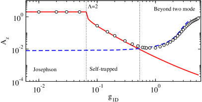
Figure 1: Maximum amplitude of the imbalance oscillations, $z_{\rm max}-z_{\rm min}$ computed with GP (circles) as a function of $g_{1D}$. The solid (red) line is the classical two-mode prediction using Eqs. (2). The dashed (blue) line is a two-mode calculation using modes (2,3) as explained in the text.

III Results

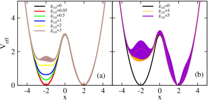
Figure 2: (color online) Effective potential $V_{\rm eff}(x,t)=V(x)+g_{1D}|\Psi(x,t)|^{2}$ for different values of $g_{1D}$. The bands are generated by joining $V_{\rm eff}(x,0)$ and $V_{\rm eff}(x,t_{z_{\rm min}})$, as explained in the text. The key to the various lines is shown in each panel.

In all the calculations, except those in section III.3, we have $\psi(x,t=0)=\Phi_{L}(x)$ (obtained by previously computing $\Phi_{1}$ and $\Phi_{2}$ of the GP for each $g_{1D}$), corresponding to the case of all atoms being on the left well, $z(0)=1$, at $t=0$. We study the dynamics for increasing values of $g_{1D}\geq 0$, going from the Rabi regime, $g_{1D}=0$, to the Josephson and self-trapped dynamics, and further beyond the range of validity of the usual two-mode approximation.

Results are shown in figure 1. There we compare the numerically determined GP amplitudes of $z(t)$, empty circles, with the semiclassical two mode prediction of Eq. (2), solid (red). At $g_{1D}<g_{1D}^{(1,2)}$ there is no self-trapping and $z(t)$ oscillates between $+1$ and $-1$, thus leading to a constant maximal amplitude, $A_{z}\equiv z_{\rm max}-z_{\rm min}=2$. With increasing interaction strength, near $g_{1D}^{(1,2)}$, self-trapping appears, the atoms become increasingly confined in the left well, and $A_{z}$ decreases abruptly. In all this range the semiclassical model predictions are very successful, covering the well known Josephson and self-trapped regimes. This range of $g_{1D}$ is the one recently explored experimentally in Ref. tilman10 .

With further increase of $g_{1D}$, deviations begin to appear. Whereas the semiclassical two-mode model predicts a smooth decrease of $A_{z}$, the GP calculations, empty circles, show a smooth reappearance of tunneling between the two wells. This is the new phenomenon that we will now discuss and interpret.

Figure 2 shows the effective potential defined in Eq. (1) for several values of $g_{1D}$ at two different times, $t=0$ and $t=t_{z_{\rm min}}$ which correspond to the time of the first minimum of the population imbalance. In this way the band covers the variation of the effective potential during the simulation. When $g_{1D}\lesssim g_{1D}^{(1,2)}$ the non-linear contribution is fairly small, and $V_{\rm eff}(x,t)\simeq V(x)$ at all times. This corresponds to the Rabi and Josephson regimes, with maximal oscillations of the population. Increasing $g_{1D}$ further, $g_{1D}^{(1,2)}\lesssim g_{1D}\lesssim 3$, the value of $V_{\rm eff}(x,t)$ in the left well is increased, but leaving the value in the right well almost unchanged. This is a direct consequence of self-trapping. In this regime, the effective potential changes very little with time, see fig. 2 (a). Further increasing $g_{1D}$, $3\lesssim g_{1D}\lesssim 5$, the potential on the left well increases, and $V_{\rm eff}$ does begin to change appreciably with time. Still, the dynamics remains self-trapped but with larger oscillation amplitudes in $z(t)$.

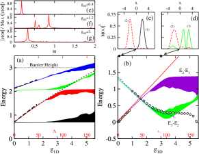
Figure 3: (a) First four eigenvalues of $V_{\rm eff}$ at $t=0$ and $t=t_{z_{\rm min}}$, thus generating the bands. The dashed black lines are the first order perturbation theory calculation described in the text. The dotted line is the average energy of the initial state, $\langle\psi(x,0)|H|\psi(x,0)\rangle$. (b) Energy differences $E_{2}-E_{1}$ (violet band) and $E_{3}-E_{2}$ (green band) compared to twice the frequencies of oscillation of the population imbalance computed with GP, empty circles. The solid (red) line is the usual two-mode calculation using Eqs. (2). The dashed (blue) line is a two-mode calculation using modes (2,3) as explained in the text. (c) and (d) depict the two relevant eigenstates of the effective potential (computed at $t=0$) entering into the dynamics for $g_{1D}=0.1$ and 3, respectively. (e), (f), and (g) depict the normalized Fourier transform of $z(t)$, $|z(\omega)|$, for $g_{1D}=0.4,1.4$ and $3$ respectively.

III.1 Analysis of the effective potential

To clarify the discussion and further gauge the smallness of the changes in the potential with time, we have determined the first four stationary solutions of the Schrödinger equation built with $V_{\rm eff}(x,t)$, with $t$ a fixed parameter. Figure 3 (a), shows the eigenvalues thus found numerically. Two values of the parameter $t$ have been chosen: $t=0$ and $t=t_{z_{\rm min}}$, to form a band for each eigenvalue. The band width is seen to remain very small for $g_{1D}\lesssim 2.2$, in line with the largely time independent $V_{\rm eff}$ depicted in Fig. 2 (a). For small interaction strengths, $g_{1D}\lesssim 2$, two of the eigenvalues are practically independent of $g_{1D}$: they correspond to states 1 and 3, mostly located in the right well, which remains unchanged as seen in Fig. 2 (a). Their values are thus close to the corresponding non-interacting harmonic oscillator, $E_{1}^{ho}=\sqrt{2}/2$ and $E_{2}^{ho}=3\sqrt{2}/2$.

The other two eigenvalues increase smoothly with the interaction strength, they correspond to states 2 and 4 located mostly in the left well. The increase follows the behavior of the effective potential shown in figure 2. The almost linear increase in energy of these two eigenvalues can be understood treating the non-linear term as a perturbation, then

$$\delta E_{2} = g_{1D}\langle\,\psi_{1}^{ho}|\,|\psi_{1}^{ho}|^{2}\,|\psi_{1}^{ho}\rangle=g_{1D}/(2^{1/4}\sqrt{\pi})\,,$$

$$\delta E_{4} = g_{1D}\langle\psi_{2}^{ho}|\,|\psi_{1}^{ho}|^{2}\,|\psi_{2}^{ho}\rangle=\delta E_{2}/2\,,$$ (4)

where $\psi_{1,2}^{ho}$ are the first two eigenfunctions of the harmonic trap, $V(x)=(x+2)^{2}$:

$$\psi_{1}^{ho}(x) = (\sqrt{2}/\pi)^{1/4}\,e^{-\sqrt{2}(x+2)^{2}\over 2}\,,$$

$$\psi_{2}^{ho}(x) = 2^{3/4}\,(x+2)\,\psi_{1}^{ho}(x)\,.$$ (5)

These estimates are shown in Fig. 3 (a) as dashed lines.

As sketched above, in the conventional two mode picture one considers only the lowest two stationary solutions of the original GP equation, (1), and self-trapping occurs due to a misalignment of their eigenenergies that suppresses the (Josephson) tunneling between the two states. The dynamics thus involves two quasi-degenerate states arising from the ground states of the unconnected wells.

III.2 Beyond the usual two-mode dynamics

What is new here is that near $g_{1D}\simeq 2$ $(\Lambda\sim 60)$, the third eigenvalue becomes aligned with the second and, since the corresponding modes are located in different wells, tunneling of atoms is again allowed. But now between modes 2 (left well) and 3 (right well). This corresponds to the rise of $A_{z}$ in figure 1 beyond $g_{1D}\simeq 1$. Figure 3a shows that by increasing the non-linear interaction we go from the usual coupling between the two lowest modes, 1 and 2, see panel (c), to a coupling of the lowest mode of the left-well, 2, to the first mode of the right well, 3, see panel (d). This coupling, which is zero in absence of interaction, occurs due to the large nonlinearity: it deforms the wave functions enough to enable the coupling between the ground state of one well and the first excitation in the other. It is a large and clearly density dependent effect which requires a change in the modes used and cannot be accommodated by varying the parameters of the usual two-mode picture. This effect is different in nature from what was reported in Refs. tonel2005 ; carr2007 ; carr2010 where the alignment takes place due to the presence of a large enough bias in the system. In our case, it is clearly a dynamical phenomenon which happens even for symmetric double-well potentials. The role played here by the non-linear interaction in modifying the single particle states is more similar to the interaction blockade effect demonstrated for double-wells with few atoms in optical superlattices cheinet08 .

Our result is also of different nature to the disappearance of self-trapping reported in Ref. meier01 . There, the authors explore the population of low-energy Bogoliubov excitations in the condensates of each of the wells finding, using a schematic model, a departure from self-trapping due to excitation of such low energy modes. By using the time-dependent GP equation to determine the condensate wavefunction, the low energy Bogoliubov states are already incorporated into its time evolution. See Eq. (8.43) and the discussion in section VIII.E in Ref. Leggett01 . Including them again along the lines of Ref. meier01 would be redundant.

To further confirm our picture, in panel (b) of figure 3 we compare the frequencies of oscillation of $z(t)$  found in the full GP calculations, shown as empty circles, to the energy differences of the first three modes . Up to $g_{1D}\simeq 1$ the two mode description with states 1 and 2 works very well, but beyond that, the appropriate two mode model must involve states 2 and 3, and tunneling between wells increases again due to the progressive alignment between the energies of these two modes. The transition from (1,2) to (2,3) takes place smoothly, with the region $1\lesssim g_{1D}\lesssim 2$ having more than one clear peak in the Fourier transform, $z(\omega)$, see panel (f) of Fig. 3, but an extremely small oscillation amplitude as seen in Fig. 1. In this region, the dynamics is governed by the first three modes coupled pairwise, (1,2) and (2,3).

Above $g_{1D}\simeq 2$, the dynamics is dominated by modes 2 and 3, depicted in panel (d) of Fig. 3. The strongest frequency extracted from the GP calculation now falls close to the $E_{3}-E_{2}$ band (green). Following similar arguments to those in the derivation of Eqs. (2) we can write down the new two mode equations: We denote the second and third modes of $V_{\rm eff}(x,0)$ as $\Phi_{L}$ and $\Phi_{R}$. A slight generalization of Eqs. (2) leads to

$$\dot{z}(t) = -2{\cal K}\sqrt{1-z^{2}(t)}\,\sin{\delta\phi(t)}$$ (6)

$$\dot{\delta\phi(t)} = \Delta+N\,\bar{U}z(t)+2{\cal K}{z(t)\over\sqrt{1-z^{2}(t)}}\,\cos{\delta\phi(t)}\,$$

where,

$$\Delta = (E_{L}^{0}-E_{R}^{0})+(U_{L}-U_{R})/2$$

$$\bar{U} = (U_{L}+U_{R})/2$$

$$U_{L(R)} = \lambda_{0}\int\!dx\,\Phi_{L(R)}^{4}$$ (7)

$$E^{0}_{L(R)} = \int dx\left((1/2)\partial_{x}\Phi_{L(R)}\partial_{x}\Phi_{L(R)}+\Phi^{2}_{L(R)}\,V(x)\right)\,.$$

Using $g_{1D}=1.2$ to build the modes gives, $\Delta=-1.26$, $\bar{U}=0.35$, and ${\cal K}=-0.037$. The prediction of this new two-mode model is shown by the dashed (blue) lines in Fig. 1 and Fig. 3(b). As can be seen this (2,3) model works well in the range $1\lesssim g_{1D}\lesssim 3.5$, giving a good account of both the dominant frequency and the amplitude of the imbalance observed in the GP simulations. The transition from (1,2) to (2,3) coupling reflects also in the appearance of the node of the $|\psi(x,t)|^{2}$ near $x=2$, obtained solving the GP equations as seen in Fig. 4. This is an observable feature which should be looked for experimentally.

Further increasing $g_{1D}$, $g_{1D}\gtrsim 6$, our initial state has an average energy above the barrier, see dotted line in Fig. 3 (a), thus facilitating the flow of atoms between the wells. At high enough $g_{1D}$ a certain equilibration of the imbalance can be expected, in line with Ref. ceder2009 , mostly due to the sizeable contributions from modes with energies above the barrier.

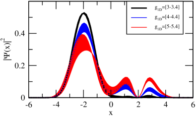
Figure 4: Density of atoms along the $x$ direction at a given time $t=t_{\rm Rabi}/10$ for several values of $g_{1D}$. The bands are built by joining the calculations at two different values of $g_{1D}$.

III.3 Critical $g_{1D}^{(2,3)}$ for $z(0)<1$

Until now we have considered only cases with a maximally imbalanced initial condition, $z(0)=1$. For other initial conditions, $z(0)<1$ we can estimate the critical value for the tunneling between modes (2,3), $g_{1D}^{(2,3)}$, using similar arguments to the ones leading to Eq. (4). The value of $g_{1D}^{(2,3)}$ for $z(0)=1$ corresponds to the one for which the second energy level (the first of the most populated well) equals the third energy level (the second of the less populated well). Thus fulfilling $E_{1}^{ho}+\delta E_{2}=E_{3}$, which can easily be solved giving, $g_{1D}^{(2,3)}=2^{3/4}\sqrt{\pi}\sim 2.98$, in good agreement with Figs. 2 and  3.

Similarly, we can estimate the critical value, $g_{1D}^{(2,3)}$, for an initial state with a certain population imbalance $z_{0}\equiv z(0)>0$. In this case, assuming the system remains mostly self-trapped, we can define the fraction of atoms on the left well, $p_{L}\equiv(1+z_{0})/2$, and on the right well, $p_{R}\equiv(1-z_{0})/2$. We can use a similar argument as before and assume the wave function of the system is essentially a harmonic oscillator wave function at each side of the trap. We assume, the left well stays mostly on the ground state, while the right side is promoted to the first excited one. Treating again the non-linearity as a perturbation, we have, ($E_{1}\equiv E_{1R}$, $E_{2}\equiv E_{1L}$, $E_{3}\equiv E_{2R}$, $E_{4}\equiv E_{2L}$),

$$\delta E_{1} = g_{1D}p_{R}\langle\psi_{1}^{ho}||\psi_{2}^{ho}|^{2}|\psi_{1}^{ho}\rangle=g_{1D}p_{R}/(2^{5/4}\sqrt{\pi})\,,$$

$$\delta E_{2} = g_{1D}p_{L}\langle\psi_{1}^{ho}||\psi_{1}^{ho}|^{2}|\psi_{1}^{ho}\rangle=g_{1D}p_{L}/(2^{1/4}\sqrt{\pi})\,,$$

$$\delta E_{3} = g_{1D}p_{R}\langle\psi_{2}^{ho}||\psi_{2}^{ho}|^{2}|\psi_{2}^{ho}\rangle=(3/2)\delta E_{1}\,,$$

$$\delta E_{4} = g_{1D}p_{L}\langle\psi_{2}^{ho}||\psi_{1}^{ho}|^{2}|\psi_{2}^{ho}\rangle=(1/2)\delta E_{2}\,.$$ (8)

The critical condition would correspond to have $E_{2}\sim E_{3}$, that is $E_{2}^{ho}+\delta E_{3}=E_{1}^{ho}+\delta E_{2}$

$${3\over\sqrt{2}}+{3\over 2}{g^{1c}_{1D}p_{R}\over 2^{5/4}\sqrt{\pi}}={1\over\sqrt{2}}+{g^{1c}_{1D}p_{L}\over 2^{1/4}\sqrt{\pi}}\,,$$ (9)

which gives,

$$g^{(2,3)}_{1D}={4\;2^{3/4}\sqrt{\pi}\over 4p_{L}-3p_{R}}\,.$$ (10)

For $p_{R}\ll 1$ we have, $g^{(2,3)}_{1D}\sim 2^{3/4}\sqrt{\pi}\left[1+(7/4)p_{R}\right]\,.$ Thus, for $z(0)$ close to 1, the critical value, $g_{1D}^{(2,3)}$, grows linearly with the initial fraction of atoms in the less populated well.

III.4 Possible experimental conditions

The phenomena presented in the previous sections rely on the adequateness of the Gross-Pitaevskii equation to describe the physics at large enough values of $g_{1D}$. The predicted reappearance of tunneling of atoms through the barrier beyond the usual self-trapped region as we increase $g_{1D}$ requires quantum fluctuations to be minimized during the whole process. Thus, we need to estimate with realistic conditions whether the system can be brought to such $g_{1D}$ values while remaining mostly condensed.

We consider $N$ atoms of ⁸⁷Rb trapped inside an axially symmetric trap, characterized by $\omega_{\perp}$, and its associated length $a_{\perp}=(\hbar/M\omega_{\perp})^{1/2}$. The double-well potential is built with a frequency $\omega_{x}$ inside each well. The scaled 1D coupling, $\hat{g}$, can be written in the weakly interacting limit  as sala02 ,

$$\hat{g}={4\pi\hbar^{2}a_{s}\over 2\pi a_{\perp}^{2}M}={2\hbar a_{s}\omega_{\perp}}\,.$$ (11)

To obtain meaningful estimates we consider the elongated trap conditions of Ref. gio08 : $\omega_{x}=2\pi 44.7$ Hz and $\omega_{\perp}=2\pi 1100$ Hz. For these we can estimate the dilution factor, $\eta=n_{1D}a_{s}$, where $a_{s}$ is the s-wave scattering length and $n_{1D}$ is the one-dimensional density. In the Thomas-Fermi limit, this estimate is given by

$$\eta=(g_{1D})^{2/3}{\omega_{x}\over\omega_{\perp}}{1\over 3^{1/3}2^{5/3}}\,,$$ (12)

and for the trap conditions considered, $\eta\sim 9\times 10^{-3}(g_{1D})^{2/3}\,.$ Thus, an elongated trap ensures the diluteness of the gas along the direction of the barrier, which is a necessary condition for the validity of the Gross-Pitaevskii approximation. The diluteness on the longitudinal direction also ensures the non-excitation of transverse modes of the elongated trap. This can be checked by comparing the transverse chemical potential with the transverse quantum, $\hbar\omega_{\perp}$. The transverse chemical potential can be written as, see Eq. (10) of  paul07 , $\mu_{\perp}=\hbar\omega_{\perp}(1+2\eta)$ which is well below $2\hbar\omega_{\perp}$ for the values of $g_{1D}$ considered in this work provided the trap is cigar-shaped.

This excitation of the third mode (the first excited state of the less-populated well) should show up macroscopically in the experiments as an increase in the amplitude of oscillations of the population imbalance above a certain value of the interaction strength. Simultaneously, a node should appear in the center of the atomic cloud sitting in the less populated well, see Fig. 4.

Experimentally, the challenge is twofold: first one needs to build a double-well potential with a single-particle spectrum close to the one described here, see Fig. 3a. This can be achieved by modifying the parameters of the optically produced double-well used in Ref. Albiez05 . Secondly, one needs to increase the number of atoms to have a non-linear term able to scan the transition described in this article. Such an experiment is within reach with current experimental setups oberp .

IV Conclusions

We have demonstrated the possibility of exciting higher modes of the double-well potential through the dynamics. We have considered an initially imbalanced population and have shown that for a broad range of interaction energies the system remains self-trapped but not due to the dynamics of the two lower states of the Gross-Pitaevskii equation, as usually accepted, but of another mechanism involving a third state. This transition from the coupling between the first two (1,2) to the next two (2,3) states can be well characterized and understood by analyzing the static properties of the effective potential (including interactions) which due to the fact that the system remains mostly self-trapped does not vary substantially with time.

- (1) A. J. Leggett, Rev. Mod. Phys. 73, 307 (2001).
- (2) C.J. Pethick and H. Smith, Bose-Einstein Condensation in Dilute Gases (Cambridge University Press, 2002).
- (3) L. Pitaevskii, and S. Stringari, Bose-Einstein Condensation. (Oxford University Press, Oxford, 2003).
- (4) R. Gati and M.K. Oberthaler, J. Phys.B: At. Mol. Opt. Phys. 40(2007)R61-R89.
- (5) M. Lewenstein, A. Sanpera, V. Ahufinger, B. Damski, A. Sen (De) and U. Sen, Adv. in Phys. 56, 243 (2007).
- (6) I. Bloch, J. Dalibard, and W. Zwerger, Rev. Mod. Phys. 80, 885 (2008).
- (7) A. Smerzi, S. Fantoni, S. Giovanazzi, S. R.Shenoy, Phys. Rev. Lett. 79, 4950 (1997).
- (8) S. Raghavan, A. Smerzi, S. Fantoni, and S. R. Shenoy, Phys. Rev. A 59, 620 (1999).
- (9) M. Albiez, R. Gati, J. Fölling, S. Hunsmann, M. Cristiani, and M. K. Oberthaler Phys. Rev. Lett. 95, 010402 (2005).
- (10) T. Zibold, E. Nicklas, C. Gross, M.K. Oberthaler, arXiv:1008.3057.
- (11) J. Esteve, C. Gross, A. Weller, S. Giovanazzi, M. K. Oberthaler, Nature 455, 1216 (2008).
- (12) C. Gross, T. Zibold, E. Nicklas, J. Esteve, M.K. Oberthaler, Nature 464, 1165 (2010).
- (13) G.J. Milburn, J. Corney, E. M. Wright, D. F. Walls, Phys. Rev. A 55, 4318 (1997).
- (14) K. Sakmann, A. I. Streltsov, O. E. Alon, and L. S. Cederbaum, Phys. Rev. Lett. 103, 220601 (2009).
- (15) D. Ananikian and T. Bergeman, Phys. Rev. A 73, 013604 (2006).
- (16) A.P. Tonel, J. Links and A. Foerster, J.Phys. A: Math. Gen. 38,6879-6891 (2005).
- (17) D.R. Dounas-Frazer, A. M. Hermundstad, L.D. Carr, Phys. Rev. Lett. 99, 200402 (2007).
- (18) L.D. Carr, D.R. Dounas-Frazer and M.A. Garcia-March, EPL 90, 10005 (2010).
- (19) P. Cheinet, S. Trotzky, M. Feld, U. Schnorrberger, M. Moreno-Cardoner, S. Fölling, and I. Bloch, Phys. Rev. Lett. 101, 090404 (2008).
- (20) F. Meier, and W. Zwerger, Phys. Rev. A 64, 033610 (2001).
- (21) L. Salasnich, A. Parola, and L. Reatto, Phys. Rev. A 65, 043614 (2002).
- (22) T. Paul, M. Hartung, K. Richter, and P. Schlagheck, Phys. Rev. A 76, 063605 (2007).
- (23) S. Giovanazzi, J. Esteve and M. K. Oberthaler, New J. of Phys. 10, 045009 (2008).
- (24) M. K. Oberthaler, private communication.