Abstract

We consider phenomenological consequences of RS2-$n$ model with infinite extra dimension, namely, the production, in high energy collisions, of a photon or $Z$-boson escaping from our brane in association with a photon remaining on the brane. This would show up as process $e^{+}e^{-}\rightarrow\gamma+\mbox{nothing}$. We compare the signal with the Standard Model background coming from $e^{+}e^{-}\rightarrow\gamma\bar{\nu}\nu$. We also make a comparison with $e^{+}e^{-}\rightarrow\gamma+\mbox{nothing}$ in the ADD model.

1 Introduction

Particle escape from our brane is a rather common feature of brane-world theories with extra dimensions of infinite size. This property has been already discussed in the context of the early toy models of brane world [1]. In $D$-brane constructions, incomplete localization of matter and gauge fields on the brane, and hence particle escape from the brane, is a characteristic of the Higgs phase [2]. Warped models [3] with the gravitational mechanism of particle (quasi-)localization on the brane [4, 5] also share the property of particle escape [6, 7]. From 4-dimensional perspective, particle escape occurs when there exists a continuum of massive modes; in multi-dimensional language, these modes correspond to particles moving away from the brane towards infinity in extra dimensions. Even though particle escape can be interpreted in purely 4-dimensional terms via adS/CFT correspondence [8, 9], in practice the escaped particles are undetectable. Their production would manifest itself as missing energy events at particle colliders.

In this paper we focus on photon and $Z$-boson escape from our brane in a model with one non-compact warped extra dimension. This model extends the original Randall–Sundrum brane-world set up [3] by the addition of $n$ compact extra dimensions [10, 11, 5, 7] (RS2-$n$ model). The latter ones are instrumental for the gravitational mechanism of (quasi-)localization of gauge fields, similar to the graviton localization in the original RS2 model. Specifically, the set up involves a $(3+n)$ — brane with $n$ compact dimensions and positive tension, embedded in a $(5+n)$-dimensional space-time with the $AdS_{5+n}$ metric:

$$ds^{2}=a(z)^{2}(\eta_{\mu\nu}dx^{\mu}dx^{\nu}-\delta_{ij}d\theta^{i}d\theta^{j})-dz^{2}\;.$$ (1)

Here $\theta_{i}$ are the coordinates of the compact extra-dimensions, $\theta_{i}\in[0,2\pi R_{i}]$, $i=1,\dots n$, and

$$a(z)=e^{-k|z|}$$

is the warp factor characteristic of the Randall-Sundrum class of models. This metric is a solution to the $(5+n)$-dimensional Einstein equations with the appropriately tuned brane tension. The $AdS_{5+n}$ curvature parameter $k$ is determined by the $(5+n)$-dimensional Planck mass and the negative bulk cosmological constant.

In the background geometry (1), massless gauge field propagating in the bulk has an exactly localized mode with zero 4-dimensional mass [5, 7]. The wave function of this mode is independent of extra-dimensional coordinates, in accord with the requirement of charge universality [12]: the 4-dimensional gauge charges of particles trapped to our brane are independent of the shapes of their wave functions in extra dimensions. On the other hand, once the gauge field obtains a mass via the Higgs mechanism (with either brane or bulk Higgs field), this would-be localized mode becomes quasi-localized on the brane, i.e., the massive vector boson has finite width against the escape into extra dimensions. In both cases, the continuum of the bulk modes starts from zero 4-dimensional mass squared.

There are both low- and high-energy manifestations of this scenario. The low-energy phenomena include invisible positronium decay [13], star cooling [14], etc., and, indeed, strong constraints on the parameter $k$ have been obtained, especially for small $n$, by considering these effects. These low-energy effects may not be generic, however, since in constructions generalizing (1), there might be a gap in the spectrum of 4-dimensional masses and/or the bulk vector boson wave functions might be strongly suppressed on the brane at low energies. One of the high energy manifestations is the invisible $Z$-boson decay [15]; we quote the corresponding constraints later on. In this paper we study yet another effect, $e^{+}e^{-}\to\gamma+\mbox{nothing}$, where “nothing” is an undetectable photon or $Z$-boson escaping into extra dimensions. Our purpose is to calculate the cross sections of this process in two versions of the model and figure out whether there are ranges of the parameter $k$ for different $n$ which would be accessible at future colliders.

The main Standard Model background to the process we discuss is $e^{+}e^{-}\to\gamma\bar{\nu}\nu$. So, we compare our signal with this background. We also make comparison with the ADD model [16] in which the emission of a Kaluza–Klein graviton also shows up as the process $e^{+}e^{-}\to\gamma+\mbox{nothing}$, which may also occur at sizeable cross section [17].

This paper is organized as follows. We begin in Section 2 with a prototype model of one massless or massive bulk vector field propagating in the background (1). We assume everywhere in this paper that fermions interacting with the vector fields are confined to our brane and consider in Section 2 vector-like interaction. We obtain the wave functions of the bulk vector bosons, evaluate the 4-dimensional effective action and arrive at the cross section of $e^{+}e^{-}\to\gamma+\mbox{nothing}$ in this prototype model. We study two versions of the Standard Model embedded into the higher-dimensional theory in Sections 3 and 4, respectively. In Section 3 we put entire $SU(2)_{W}\times U(1)_{Y}$ gauge sector, as well as the Higgs sector, into the bulk. This version is a straightforward generalization of the model of Section 2. In Section 4 we assume that only $U(1)_{Y}$ part of the Standard Model gauge theory lives in the bulk, and that the Higgs field is localized on the brane. Although physics is somewhat different in this model, the results are qualitatively similar to those of Section 3. In Section 5 we derive the bounds on the parameter $k$ for various $n$, which are based on the measurement of the invisible $Z$-decay width, and give comparison of $e^{+}e^{-}\to\gamma+\mbox{nothing}$ in the two models with the Standard Model $e^{+}e^{-}\to\gamma\bar{\nu}\nu$ and the ADD process $e^{+}e^{-}\to\gamma+\mbox{KK\leavevmode\nobreak\ graviton}$. We conclude in Section 6.

2 Prototype model

2.1 Wave functions in extra dimensions

We begin with a model of one bulk vector field $B_{A}$ coupled to fermions localized on the brane. The action in the background metric (1) has the following form:

$$S=\int\prod^{n}_{i=1}\dfrac{d\theta_{i}}{2\pi R_{i}}\,dz\,d^{4}x\sqrt{|g|}\,\left(-\frac{1}{4}g^{AC}g^{BD}F_{AB}F_{CD}+\frac{M_{5}^{2}}{2}g^{AB}B_{A}B_{B}\right)$$ (2)

where the indices $A,B,C,D$ run from $0$ to $(3+1+n)$, and $F_{CD}=\partial_{C}B_{D}-\partial_{D}B_{C}$. The interaction of the vector field with fermions is described by action:

$$S_{int}=g_{5}\int\prod^{n}_{i=1}\dfrac{d\theta_{i}}{2\pi R_{i}}\,dz\,d^{4}x\sqrt{g}\,\delta(z)\bar{\psi}(x)\gamma^{\mu}B_{\mu}(x,z)\psi(x)$$ (3)

where the index $\mu$ runs from $0$ to $3$ and $g_{5}$ is the coupling constant of dimension $m^{-1/2}$.

We consider the case where the energy of colliding particles is smaller than $k$, and assume that $R_{i}\lesssim k^{-1}$. Thus, at low energies, $E\ll 1/R_{i}$, the relevant vector field modes are independent of $\theta_{i}$. We integrate the action (2), (3) over coordinates of the compact extra dimensions and obtain the effective 5-dimensional action for these modes:

$$S=\int d^{4}x\,dz\,a^{n+4}\,\left(-\frac{1}{4}g^{ac}g^{bd}F_{ab}F_{cd}+\frac{M_{5}^{2}}{2}g^{ab}B_{a}B_{b}\right)+\\ +g_{5}\int d^{4}x\,dz\,\delta(z)\,\bar{\psi}(x)\gamma^{\mu}B_{\mu}(x,z)\psi(x)$$ (4)

where the indices $a,b,c,d$ run from $0$ to $(3+1)$. We now solve the classical equations of motion for the vector field in the background metric (1), which follow from action (4):

$$\frac{1}{\sqrt{|g|}}\partial_{c}(\sqrt{|g|}g^{ac}g^{bd}F_{ab})+M_{5}^{2}B^{d}=0\;.$$ (5)

We do that separately for massless and massive bulk vector fields.

2.1.1 Massless bulk vector field

First, we consider the case of zero bulk mass, $M_{5}=0$, and reproduce the results of Ref. [7] (for a review see, e.g., Ref. [18]). Let us fix the gauge $B_{z}=0$. Then Eq. (5) reduces to two equations,

$$\frac{1}{a^{2}}\partial_{\mu}F_{\mu\nu}-\frac{1}{a^{n+2}}\partial_{z}(a^{n+2}\partial_{z}B_{\nu})=0$$ (6)

$$\partial_{\mu}\partial_{z}B_{\mu}=0$$ (7)

These equations describe a localized mode and a continuous spectrum of massive excitations. The localized mode obeys

$$\partial_{z}B_{\mu}=0\;,$$ (8)

so Eq. (6) becomes the Maxwell equation for free electromagnetic field. Thus, the wave function of the localized mode is independent of $z$. Nevertheless, it is normalizable, since the appropriate weight is $a^{n}(z)dz$, see (4). We refer to this solution as $A_{\mu}$ in order to distinguish it from non-localized ones discussed below.

The second type of solutions corresponds to the continuous spectrum of excitations, which are not localized on the brane. From the 4-dimensional viewpoint they have non-zero masses. In the 4-dimensional momentum representation, the solutions even under reflection of $z$ are

$$B_{\mu}(p,z)=B_{\mu}(p,m)\Psi(z,m)\;,$$ (9)

with

$$\Psi(z,m)=C_{m}e^{(\frac{n}{2}+1)k|z|}\left(\eta_{m}J_{\frac{n}{2}+1}\left(\frac{m}{k}e^{k|z|}\right)+N_{\frac{n}{2}+1}\left(\frac{m}{k}e^{k|z|}\right)\right)$$ (10)

and

$$\eta_{m}=-\dfrac{N_{\frac{n}{2}}(\frac{m}{k})}{J_{\frac{n}{2}}(\frac{m}{k})}\;,$$ (11)

where $p^{2}=m^{2}$, $B_{\mu}(p,m)$ is transverse in 4-dimensional sense, $p^{\mu}B_{\mu}(p)=0$, and $C_{m}$ is the normalization constant. Other possible modes, which are odd under reflection of $z$, do not interact with fermions, and thus are of no interest.

One way to obtain the normalization condition is to consider the energy integral,

$$E=\int d^{4}x\,dz\,T^{0}_{0}\sqrt{|g|}$$ (12)

where $T^{0}_{0}$ is the energy-momentum tensor derived from the action (2). We substitute here the expansion of the field $B_{\mu}(x,z)$ in creation and annihilation operators,

$$B_{\mu}(x,z)=\int_{0}^{\infty}dm\int\frac{d^{3}p}{(2\pi)^{3}}\cdot\frac{\Psi(z,m)}{\sqrt{2E_{p,m}}}\sum_{\alpha}\left(a^{\alpha+}_{p,m}e^{ipx}+a^{\alpha}_{p,m}e^{-ipx}\right)e^{\alpha}_{\mu}(p)\,,$$ (13)

and require that the energy has the standard form

$$E=\int_{0}^{\infty}dm\int d^{3}p\,E_{p,m}\sum_{\alpha}a^{\alpha+}_{p,m}a^{\alpha}_{p,m}\,.$$ (14)

In this way we obtain the following normalization condition:

$$\int dza^{n}\Psi(z,m)\Psi(z,m^{\prime})=\delta(m-m^{\prime})\;,$$ (15)

which gives

$$C_{m}=\sqrt{\frac{m}{2k(\eta_{m}^{2}+1)}}\;.$$ (16)

Although the normalization condition (15) is obvious, the above way to derive it is quite general, and will be used below in less trivial situations.

By performing the integration in (2) over the coordinate of extra dimension $z$ and taking into account the normalization condition (15), we obtain the following expression for the effective 4-dimensional action in the case $M_{5}=0$:

$$S_{eff}=-\frac{1}{4}\int d^{4}x\,\mathcal{F}_{\mu\nu}\mathcal{F}_{\mu\nu}+g_{4}\int d^{4}x\,A_{\mu}\bar{\psi}\gamma_{\mu}\psi+\\ +\int dm\,d^{4}x\left(-\frac{1}{4}F_{\mu\nu}(x,m)F_{\mu\nu}(x,m)+\frac{m^{2}}{2}B_{\mu}(x,m)B_{\mu}(x,m)\right)+\\ +g_{5}\int dm\,\Psi(0,m)\int d^{4}x\,B_{\mu}(x,m)\bar{\psi}\gamma^{\mu}\psi$$ (17)

The first two terms here represent massless vector field (8) localized on the brane. The effective 4-dimensional and 5-dimensional couplings are related by

$$g_{4}=g_{5}\cdot\sqrt{\frac{kn}{2}}\;,$$ (18)

where the factor $\sqrt{\frac{kn}{2}}$ emerges due to the integration over $z$. The interaction of massive modes in (17) is suppressed at $m\ll k$ by their wave functions at the brane position,

$$\Psi(0,m)=\frac{2}{n\Gamma(\frac{n}{2})}\cdot\left(\frac{m}{2k}\right)^{\frac{n-1}{2}}\;$$ (19)

It follows from (17) that the phase space volume element for modes from the continuous spectrum is

$$d\omega=\dfrac{1}{2E_{{\bf{p}},m}}\dfrac{d^{3}p}{(2\pi)^{3}}dm,\qquad E_{{\bf{p}},m}=\sqrt{m^{2}+{\bf{p}}^{2}}$$ (20)

2.1.2 Massive field

Now let us turn to the massive bulk vector field, and focus on the case

$$M_{5}\ll k\;.$$

Equation (5) now gives the following two equations:

$$\frac{1}{a^{2}}(\partial^{2}_{\mu}B_{\nu}-\partial_{\nu}\partial_{\mu}B_{\mu}))+k(n+2)\mbox{sign}(z)\partial_{z}B_{\mu}-\partial^{2}_{z}B_{\nu}+M_{5}^{2}B_{\nu}=\\ =k(n+2)\mbox{sign}(z)\partial_{\nu}B_{z}-\partial_{\nu}\partial_{z}B_{z}$$ (21)

$$\partial_{z}\partial_{\mu}B_{\mu}=\partial_{\mu}\partial_{\mu}B_{z}+M_{5}^{2}a^{2}(z)B_{z}$$ (22)

These equations have transverse and longitudinal solutions in 4-dimensional sense. Transverse solutions obeying $\partial_{\mu}B_{\mu}=0$ have the following form:

$$B_{\mu}(p,z)=B_{\mu}(p,m)\,\Psi(z,m)\;,\;\;\;\;\;B_{z}=0\;,$$

where $p^{2}=m^{2}$,

$$\Psi(z,m) = \sqrt{\frac{m}{2k(\chi_{m}^{2}+1)}}\cdot e^{k(\frac{n}{2}+1)|z|}\left(\chi_{m}J_{\nu}\left(\frac{m}{k}e^{k|z|}\right)+N_{\nu}\left(\frac{m}{k}e^{k|z|}\right)\right)$$ (23)

$$\nu = \sqrt{\left(\frac{n}{2}+1\right)^{2}+\frac{M_{5}^{2}}{k^{2}}}$$ (24)

$$\chi_{m} = -\frac{(\frac{n}{2}+1-\nu)N_{\nu}(\frac{m}{k})+\frac{m}{k}N_{\nu-1}(\frac{m}{k})}{(\frac{n}{2}+1-\nu)J_{\nu}(\frac{m}{k})+\frac{m}{k}J_{\nu-1}(\frac{m}{k})}$$ (25)

Here we have used the normalization condition (15). For completeness, we also present the longitudinal solution:

$$B_{z} = \bar{C}_{m}e^{(\frac{n}{2}+1)|z|}\left(\chi_{m}J_{\nu}\left(\frac{m}{k}e^{k|z|}\right)+N_{\nu}\left(\frac{m}{k}e^{k|z|}\right)\right)$$ (26)

$$B_{\mu} = \partial_{\mu}\phi$$ (27)

$$\partial_{z}\phi = \left(1-\frac{M^{2}\,a^{2}(z)}{p^{2}}\right)B_{z}$$ (28)

Here $\bar{C}_{m}$ is the normalization constant and $\nu$ is given by (24). The longitudinal modes do not interact with fermions (this is also true in the extensions of the Standard Model we discuss in Sections 3 and 4), so we ignore them in what follows.

After integrating over the coordinate of extra dimension $z$ we obtain the following expression for the effective four-dimensional action for the transverse massive bulk vector field:

$$S_{eff}=\int dm\,d^{4}x\left(-\frac{1}{4}B_{\mu\nu}(x,m)B_{\mu\nu}(x,m)+\frac{m^{2}}{2}B_{\mu}(x,m)B_{\mu}(x,m)\right)+\\ +g_{5}\int dm\,\Psi(0,m)\int d^{4}x\,B_{\mu}(x,m)\bar{\psi}\gamma^{\mu}\psi$$ (29)

Figure 1: Quasi-localization of massive vector particle: relative weight $\chi_{m}$ in (23) and wave fiunction at the brane position $\Psi(m,0)$.

In the case of massive bulk vector field, there is no bound state analogous to (8), i.e., the massive field is not localized on the brane in the strict sense. Rather, it is quasi-localized on the brane. This effect is similar to that studied in Ref [6] for massive scalar field. One way to describe it is to notice that the wave function at the brane position, and hence the interaction term in the effective 4-dimensional action (29) strongly depends on the 4-dimensional mass,

$$\Psi^{2}(0,m)=\frac{\Gamma^{2}(\frac{n}{2}+1)}{\pi^{2}(1+\chi^{2}_{m})}\cdot\left(\frac{m}{2k}\right)^{-n-1}=\frac{n^{2}}{4}\cdot\frac{m^{4}}{\Gamma^{2}(\frac{n}{2})}\cdot\left(\frac{m}{2k}\right)^{n-1}\frac{1}{(m^{2}-M^{2}_{4})^{2}+m^{2}\Gamma_{RS}^{2}},$$ (30)

where

$$M_{4}=M_{5}\sqrt{\frac{n}{n+2}}\;,\quad\;\;\;\Gamma_{RS}=\frac{2\pi}{n\Gamma^{2}\left(\frac{n}{2}\right)}m\left(\frac{m}{2k}\right)^{n}\;.$$ (31)

This is shown in Fig. 1. The resonance at $m=M_{4}$ corresponds precisely to the quasi-localized vector particle of 4-dimensional mass $M_{4}$ and invisible width $\Gamma_{RS}(M_{4})$. Note that in the limit $k\rightarrow\infty$, one has $\Gamma_{RS}\rightarrow 0$, and $\Psi^{2}(0,m)$ tends to the delta function:

$$\Psi^{2}(0,m)\to\frac{nk}{2}\cdot\frac{1}{\pi}\frac{\Gamma_{RS}}{2}\frac{1}{(m-M_{4})^{2}+\left(\frac{\Gamma_{RS}}{2}\right)^{2}}\rightarrow\frac{nk}{2}\cdot\delta(m-M_{4}).$$ (32)

This shows that the relation (18) between the couplings remains valid at $M_{4}\ll k$. Away from the resonance, the wave functions at the brane position are still given by (19).

2.2 Annihilation into photon and nothing

Now let us evaluate the cross-section of fermion-antifermion annihilation into a photon localized on the brane and invisible vector boson escaping from the brane. Here we make use of the effective actions (17), (29) for bulk vector bosons, while the photon is described by the standard electromagnetic action. The relevant diagrams are shown in Fig. 2. The amplitude is given by

Figure 2: $\bar{e^{-}}e^{+}\rightarrow\gamma+nothing$

$$i\mathcal{M}=\overline{v}(p_{2})(-ig_{5}\gamma^{\mu})\frac{(\hat{p}_{1}-\hat{q})}{(p_{1}-q)^{2}}\tilde{e}_{\mu}(\tilde{q})(-ie\gamma^{\nu})u(p_{1})\Psi(0,m)e_{\nu}(q)+\\ +\overline{v}(p_{2})(-ig_{5}\gamma^{\mu})\frac{(\hat{q}-\hat{p}_{2})}{(q-p_{2})^{2}}e_{\mu}({q})(-ie\gamma^{\nu})u(p_{1})B_{m}(0)\tilde{e}_{\nu}(\tilde{q}),$$ (33)

where $p_{1}$ and $p_{2}$ are the momenta of the fermion and antifermion, respectively, $q$ and $\tilde{q}$ are the momenta of the photon and vector boson, $e_{\mu}$ and $\tilde{e}_{\mu}$ are their polarization vectors.

We make use of the expression (20) for the phase space volume element and obtain the differential cross section in the rest frame of fermions,

$$\frac{d\sigma}{dx\,dy}=\frac{g_{5}^{2}\,e^{2}}{8\pi}\cdot|\Psi(0,M)|^{2}\cdot\frac{1}{s}\cdot f(x,y)\;,$$ (34)

where

$$f(x,y)=\frac{1}{x\sqrt{1-x}}\cdot\frac{(2-x)^{2}+x^{2}y^{2}}{1-y^{2}}\;.$$ (35)

Hereafter

$$x=2q/\sqrt{s}\;,\quad\;\;y=\cos\theta\;,$$ (36)

where $\theta$ is the angle between the photon and beam directions, $M=\sqrt{s(1-x)}$ is the 4-dimensional mass of the invisible vector boson.

As an example, let us consider electrodynamics with the bulk electromagnetic field and brane electrons. This is precisely the theory of Section 2.1.1. We identify $g_{4}$ entering (18) with $e$, make use of (19) and obtain

$$\frac{d\sigma}{dx\,dy}=\frac{4\alpha^{2}}{\pi ns}\cdot\frac{1}{\sqrt{1-x}}\cdot\frac{1}{J^{2}_{\frac{n}{2}}(\frac{M}{k})+N^{2}_{\frac{n}{2}}(\frac{M}{k})}\cdot f(x,y)$$ (37)

In the limit $s\ll k$ we obtain the following expression

$$\frac{d\sigma}{dx\,dy}=\frac{4\pi\alpha^{2}}{n\Gamma^{2}(\frac{n}{2})}\cdot\frac{1}{s}\cdot\left(\frac{\sqrt{s}}{2k}\right)^{n}\cdot(1-x)^{\frac{n}{2}}\cdot f(x,y)$$ (38)

The cross section rapidly grows with energy for $\sqrt{s}\ll k$, which is a common property of multi-dimensional theories.

3 $SU(2)_{W}\times U(1)_{Y}$ in the bulk

Let us now consider $(4+1+n)$-dimensional $SU(2)_{W}\times U(1)_{Y}$ gauge theory with bulk gauge fields $A^{\alpha}_{M}$, $B_{M}$ and bulk Higgs field $\Phi$ in the background metric (1). We still assume that fermions are localized on the brane. The action of this theory is

$$S=\int d^{4}x\,dz\prod^{n}_{i=1}\frac{d\theta_{i}}{2\pi R_{i}}\sqrt{g}\left[-\frac{1}{4}\left(F^{\alpha}_{MN}\right)^{2}-\frac{1}{4}B^{2}_{MN}+\left(D_{M}\Phi\right)^{\dagger}D_{M}\Phi-V(\Phi^{\dagger},\Phi)+\delta(z)\mathcal{L}_{f}\right],$$ (39)

where $\mathcal{L}_{f}$ is the fermion Lagrangian (we neglect fermion masses below):

$$\mathcal{L}_{f}=i\bar{L}\left(\hat{\partial}-i\widetilde{g}_{1}\frac{Y_{L}}{2}\hat{B}-i\widetilde{g}\frac{\sigma_{\alpha}}{2}A^{\alpha}\right)L+i\bar{r}\left(\hat{\partial}-i\widetilde{g}_{1}\frac{Y_{R}}{2}\hat{B}\right)r+\\ +i\bar{Q}\left(\hat{\partial}-i\widetilde{g}_{1}\frac{Y^{Q}_{L}}{2}\hat{B}-i\widetilde{g}\frac{\sigma_{\alpha}}{2}A^{\alpha}\right)Q+i\bar{q}\left(\hat{\partial}-i\widetilde{g}_{1}\frac{Y^{q}_{R}}{2}\hat{B}\right)q\;.$$ (40)

Here $\widetilde{g}$ and $\widetilde{g}_{1}$ are the $SU(2)_{L}\times U(1)_{Y}$ bulk couplings, $L$ and $r$ denote lepton doublets and singlets respectively, $Q$ and $q$ are analogous quark structures, and $V(\Phi^{\dagger},\Phi)$ is the Higgs potential,

$$V(\Phi^{\dagger},\Phi)=\frac{\tilde{\lambda}}{2}\left(\Phi^{\dagger}\Phi-\frac{v^{2}}{2}\right)^{2}\;.$$ (41)

The covariant derivative is, as usual, $D_{M}\Phi=\partial_{M}\Phi-i\frac{\widetilde{g}_{1}}{2}\hat{B}_{M}\Phi-i\widetilde{g}\frac{\sigma_{\alpha}}{2}A^{\alpha}_{M}\Phi$. The quadratic action for the vector fields in the Higgs vacuum is obtained precisely in the same way as in the 4-dimensional Standard Model. We make the usual redefinition of the gauge fields,

$$Z_{M}=\frac{1}{\sqrt{\widetilde{g}^{2}_{1}+\widetilde{g}^{2}}}\left(-\widetilde{g}_{1}B_{M}+\widetilde{g}A^{3}_{M}\right),\quad A_{M}=\frac{1}{\sqrt{\widetilde{g}^{2}_{1}+\widetilde{g}^{2}}}\left(\widetilde{g}B_{M}+\widetilde{g}_{1}A^{3}_{M}\right),$$

$$W_{M}^{\pm}=\frac{1}{\sqrt{2}}\left(A_{M}^{1}\mp iA_{M}^{2}\right)$$

and write

$$\begin{split}S&=\int d^{4}x\,dz\prod^{n}_{i=1}\frac{d\theta_{i}}{2\pi R_{i}}\sqrt{g}\Bigl{[}-\frac{1}{2}|\,W_{MN}\,|^{2}+m^{2}_{W}|\,W_{M}\,|^{2}-\frac{1}{4}Z^{2}_{MN}+\frac{1}{2}m^{2}_{Z}Z^{2}_{M}\\ &\qquad\qquad\qquad\qquad\qquad-\frac{1}{4}F^{2}_{MN}+\delta(z)\mathcal{L}_{f}\Bigr{]},\end{split}$$ (42)

where

$$m_{W}^{2}=\frac{1}{4}\widetilde{g}^{2}v^{2}\;,\qquad m_{Z}^{2}=\frac{1}{4}(\widetilde{g}^{2}+\widetilde{g}_{1}^{2})v^{2}$$

are the bulk masses of the gauge fields, while photon remains massless in the bulk. $\mathcal{L}_{f}$ is the fermion Lagrangian:

$$\mathcal{L}_{f}=\mathcal{L}_{f,em}+\mathcal{L}_{f,weak}$$ (43)

where

$$\mathcal{L}_{f,em}=g_{5}\sum_{f}q_{f}\bar{f}\gamma^{\mu}A_{\mu}f,$$ (44)

and

$$\mathcal{L}_{f,weak}=\frac{\widetilde{g}}{2\sqrt{2}}\left(\bar{\nu}\gamma^{\mu}(1-\gamma^{5})W^{+}_{\mu}e+h.c.\right)+\frac{\widetilde{g}}{2\sqrt{2}}\left(\bar{u}\gamma^{\mu}(1-\gamma^{5})W^{+}_{\mu}d+h.c.\right)$$ (45)

$$+\frac{\widetilde{g}}{2\cos\theta_{W}}\sum_{f}\bar{f}\gamma^{\mu}\left(t^{f}_{3}(1-\gamma^{5})-2q_{f}\sin^{2}\theta_{W}\right)fZ_{\mu}\;.$$

Here $g_{5}=e\sqrt{\frac{2}{nk}}=\widetilde{g}\sin\theta_{W}=\widetilde{g}_{1}\cos\theta_{W}$ is the bulk electric charge, and $eq_{f}$ is the fermion electric charge. Note that the relation (18) between 4-dimensional and multi-dimensional couplings is valid for both gauge groups, so $\sin\theta_{W}$ is expressed in terms of the 4-dimensional gauge couplings in the standard way.

3.1 Cross section of $e^{+}e^{-}\to\gamma+\mbox{nothing}$

We see that the model under discussion is a straightforward modification of the model of Section 2. In particular, the spectrum and the wave functions of the bulk vector bosons are the same as in Section 2.1.

We consider the process with the $e^{+}\,e^{-}$-pair in the initial state and with brane photon and bulk $Z$-boson in the final state. The differential cross-section for this process is

$$\frac{d\sigma}{dxdy}\left(e^{+}e^{-}\rightarrow Z_{bulk}\gamma\right)=\frac{2\alpha^{2}}{\pi nk^{2}}\cdot\frac{(-\frac{1}{2}+\sin^{2}\theta_{W})^{2}+\sin^{4}\theta_{W}}{\sin^{2}\theta_{W}\cos^{2}\theta_{W}}\cdot\\ \cdot\frac{\sqrt{1-x}}{\left((\frac{n}{2}+1-\nu)J_{\nu}(\frac{M}{k})+\frac{M}{k}J_{\nu-1}(\frac{M}{k})\right)^{2}+\left((\frac{n}{2}+1-\nu)N_{\nu}(\frac{M}{k})+\frac{M}{k}N_{\nu-1}(\frac{M}{k})\right)^{2}}\cdot f(x,y)$$ (46)

$$\nu=\sqrt{\left(\frac{n}{2}+1\right)^{2}+\frac{n+2}{2}\left(\frac{M_{Z}}{k}\right)^{2}},\quad M=\sqrt{s(1-x)}$$

In the limit $s\ll k$ we obtain

$$\frac{d\sigma}{dxdy}\left(f\bar{f}\rightarrow Z_{bulk}\gamma\right)=\frac{\pi\alpha^{2}}{s\;n\Gamma^{2}\left(\frac{n}{2}\right)}\cdot\frac{8\sin^{4}\theta_{W}-4\sin^{2}\theta_{W}+1}{\sin^{2}\theta_{W}\cos^{2}\theta_{W}}\cdot\left(\frac{\sqrt{s}}{2k}\right)^{n}\cdot\\ \cdot\frac{(1-x)^{2}}{(1-x-\frac{M^{2}_{Z}}{s})^{2}+\frac{M^{2}_{Z}\Gamma_{RS}^{2}}{s^{2}}}\cdot f(x,y)\;.$$ (47)

Here $M_{Z}$ is the four-dimensional $Z$-boson mass, and $\Gamma_{RS}$ is given by (31). Other notations are the same as in (35), (36). The $x$-dependent factor in the last part of the formula (47) comes from the squared wave function at the brane position, see (30).

The total cross section of $e^{+}e^{-}\to\gamma+\mbox{nothing}$ is the sum

$$\frac{d\sigma}{dxdy}\left(f\bar{f}\rightarrow\gamma+\mbox{nothing}\right)=\frac{d\sigma}{dxdy}\left(f\bar{f}\rightarrow Z_{bulk}\gamma\right)+\frac{d\sigma}{dxdy}\left(f\bar{f}\rightarrow\gamma_{bulk}\gamma\right)\;,$$ (48)

where the first term is given by (47) and the second term is the cross section of the production of bulk photon which is given by (38).

4 $SU(2)_{brane}\times U(1)_{bulk}$

In this Section we consider a model with localized fermions, the Higgs field localized on the brane and $SU(2)_{brane}\times U(1)_{bulk}$ gauge group. So, among all fields of the Standard Model, only $U(1)_{Y}$ gauge field propagates in extra dimensions. An interesting feature of this model is that after spontaneous symmetry breaking, the set of fields consists of the localized on the brane photon $A_{\mu}$ and quasi-localized $B_{\mu}$ instead of $Z_{\mu}$. Nevertheless, the Standard Model is restored in the limit $k\rightarrow\infty$.

Let us begin with the effective action for this theory. After integrating out compact extra dimensions, the action for this model is written as follows:

$$S=\int d^{4}xdza^{n+4}\left(\left((D_{\mu}\phi)^{+}D_{\mu}\phi-\frac{1}{4}F_{\mu\nu}^{\alpha}F_{\mu\nu}^{\alpha}-\lambda(\phi^{+}\phi-\frac{v^{2}}{2})\right)\delta(z)-\frac{1}{4}g^{MA}g^{NB}B_{MN}B_{AB}\right)$$ (49)

Here $B_{M}(x,z)$ is the $U(1)_{Y}$ gauge field, $A^{\alpha}_{\mu}(x)$, $\alpha=1,2,3$ are the $SU(2)_{brane}$ gauge fields, $F^{\alpha}_{\mu\nu}=\partial_{\mu}A^{\alpha}_{\nu}-\partial_{\nu}A_{\mu}^{\alpha}+g\varepsilon^{\alpha bc}A^{b}_{\mu}A^{c}_{\nu}$, $D_{\mu}\phi=\partial_{\mu}\phi-\frac{g}{2}\tau_{\alpha}A_{\mu}^{\alpha}-\frac{g^{\prime}}{2}\sqrt{\frac{2}{kn}}B_{\mu}(x,0)$. When writing the last expression we have recalled the relationship (18) between the multi-dimensional and 4-dimensional couplings.

After spontaneous symmetry breaking, the linearized field equations for electrically neutral vector fields are

$$\partial_{z}\partial_{\mu}B_{\mu}=0$$ (50)

$$\frac{1}{a^{2}}\partial_{\mu}\partial_{\mu}B_{\nu}-\partial_{z}^{2}B_{\nu}+(n+2)ksign(z)\partial_{z}B_{\nu}=\frac{2v^{2}g^{\prime}}{8}\sqrt{\frac{2}{kn}}\left(g^{\prime}\sqrt{\frac{2}{kn}}B_{\nu}-gA^{3}_{\nu}\right)\delta(z)$$ (51)

$$\partial_{\mu}F_{\mu\nu}+\frac{2gv^{2}}{8}\left(gA_{\nu}^{3}-g^{\prime}\sqrt{\frac{2}{kn}}B_{\nu}(x,0)\right)=0$$ (52)

Here we use the gauge $B_{z}=0$. The equations for $W^{\pm}$ bosons have the standard four-dimensional form, so we do not consider them. Equations (51), (52) have a peculiarity: since the Higgs mechanism operates on the brane, there is an additional boundary condition on the brane.

Let us first consider the case $A^{3}_{\mu}(x)=\frac{g^{\prime}}{g}\sqrt{\frac{2}{kn}}B_{\nu}(x,0)$. Equations (50)-(52) take the following form

$$\partial_{\mu}F_{\mu\nu}=0$$ (53)

$$g^{\prime}B^{\prime}_{\nu}-gA^{3}_{\nu}=0$$ (54)

$$\frac{1}{a^{2}}\partial_{\mu}\partial_{\mu}B_{\nu}-\partial_{z}^{2}B_{\nu}+(n+2)ksign(z)\partial_{z}B_{\nu}=0$$ (55)

$$\partial_{\mu}\partial_{z}B_{\mu}=0$$ (56)

Equation (53) has a solution with non-zero mass only if it is longitudinal, $A^{3}_{\mu}=p_{\mu}b(p)$, but such a solution is incompatible with Eqs. (54)-(56) for $p^{2}\neq 0$. Thus, Eqs.(53)-(56) describe a massless particle. We have shown in Section 2.1 that massless solution to equations (54),(56) is localized on the brane. So Eqs. (53)-(56) describe the photon field $A_{\mu}$. The fields $B_{\mu}$, $A^{3}_{\mu}$ are related to $A_{\mu}$ as follows

$$B_{\mu}(p,z)=\sqrt{\tfrac{kn}{2}}\tfrac{g}{\sqrt{{g^{\prime}}^{2}+g^{2}}}\cdot A_{\mu}(p)$$ (57)

$$A^{3}_{\mu}(p)=\tfrac{g^{\prime}}{\sqrt{{g^{\prime}}^{2}+g^{2}}}\cdot A_{\mu}(p)$$ (58)

The other case is $A^{3}_{\mu}(x)\neq\frac{g^{\prime}}{g}\sqrt{\frac{2}{kn}}B_{\nu}(x,0)$. The situation here is more complicated than the previous one. Equation (51) can be rewritten as bulk equation and boundary condition on the brane:

$$\frac{1}{a^{2}}\partial_{\mu}\partial_{\mu}B_{\nu}-\partial_{z}^{2}B_{\nu}+(n+2)ksign(z)\partial_{z}B_{\nu}=0$$ (59)

$$\left.\partial_{z}B_{\nu}\right|_{z\rightarrow+0}-\left.\partial_{z}B_{\nu}\right|_{z\rightarrow-0}=\frac{2g^{\prime}v^{2}}{8}\sqrt{\frac{2}{kn}}\left(gA_{\nu}^{3}-g^{\prime}\sqrt{\frac{2}{kn}}B_{\nu}\right)$$ (60)

Eqs. (59), (50) are the same as in the case of the bulk-massless vector field that was discussed in Section 2.1. Therefore we use the solution (9), (10) for the field $B_{\mu}(x,z)$, but the presence of the boundary condition (60) leads to the different expression for $\eta_{m}$. $\eta_{m}$ and $A^{3}_{\mu}$ are obtained from Eqs. (52), (60):

$$\eta_{m}=-\frac{-\frac{2m{g^{\prime}}^{2}}{kn}N_{\nu}(\frac{m}{k})+2\left(\frac{4m^{2}}{v^{2}}-g^{2}\right)N_{\nu-1}(\frac{m}{k})}{-\frac{2m{g^{\prime}}^{2}}{kn}J_{\nu}(\frac{m}{k})+2\left(\frac{4m^{2}}{v^{2}}-g^{2}\right)J_{\nu-1}(\frac{m}{k})},\quad\nu=\frac{n}{2}+1$$ (61)

$$A_{\mu}^{3}(p,m)=-B_{\mu}(p,m)\Psi(0,m)\frac{gg^{\prime}v^{2}\sqrt{\frac{2}{kn}}}{4m^{2}-v^{2}g^{2}}$$ (62)

where $\Psi(0,m)$ and $B_{\mu}(p,m)$ have the same form as in (10) and (9) respectively with $\eta_{m}$ given by (61). The normalization constant for this solution has been straightforwardly obtained by making use of the approach outlined in Section 2.1.1. It is worth noting that $\Psi(0,m)$ has the following explicit form

$$\Psi(0,m)=(m^{2}-M^{2}_{W})\widetilde{\Psi}(0,m)$$ (63)

$$\widetilde{\Psi}(0,m)=\sqrt{\frac{m}{2k}}\frac{2\left(J_{\nu-1}(\tfrac{m}{k})N_{\nu}(\tfrac{m}{k})-N_{\nu-1}(\tfrac{m}{k})J_{\nu}(\tfrac{m}{k})\right)}{\sqrt{\left((m^{2}-M_{W}^{2})J_{\nu-1}(\tfrac{m}{k})-\tfrac{m}{kn}\mathop{\rm tg}\nolimits^{2}\theta_{W}M^{2}_{W}J_{\nu}(\tfrac{m}{k})\right)^{2}+(J_{\nu}\rightarrow N_{\nu})^{2}}}\,.$$ (64)

Thus, there is no pole in (62) at $m=M_{W}=\tfrac{g^{2}v^{2}}{4}\,$.

In order to illustrate how the the massive vector fields are quasi-localized in this theory, we write the following expressions for the fields $A_{\mu}$, $Z_{\mu}$ at the brane position,

$$Z_{\mu}(p,m)=\tfrac{1}{\sqrt{g^{2}+{g^{\prime}}^{2}}}\cdot\left(gA^{3}_{\mu}(p,m)-g^{\prime}\sqrt{\tfrac{2}{kn}}B_{\mu}(p,m)\right)=m^{2}\sin{\theta_{W}}\cdot B_{\mu}(p,m)\widetilde{\Psi}(0,m)$$ (65)

$$A_{\mu}(p,m)=\tfrac{1}{\sqrt{g^{2}+{g^{\prime}}^{2}}}\left(g^{\prime}A^{3}_{\mu}(p,m)+g\sqrt{\tfrac{2}{kn}}B_{\mu}(p,m)\right)=(m^{2}-M_{Z}^{2})\cos{\theta_{W}}\cdot B_{\mu}(p,m)\widetilde{\Psi}(0,m)$$ (66)

Figure 3: $A_{\mu}$, $Z_{\mu}$, $\eta_{m}$ as functions of $m$

It is worth noting that $Z_{\mu}(p,m)$ as function of $m$, which is plotted in Fig.3, has a peak at $m=M_{Z}$ and the position of this peak corresponds to the zero of $A_{\mu}(p)$. The width $\Gamma_{RS}$ of this peak is obtained from Eqs. (64), (65) and is given by

$$\Gamma_{RS}(M_{Z})=\frac{2\pi M_{Z}\sin^{2}\theta_{W}}{n\Gamma^{2}(\tfrac{n}{2})}\left(\frac{M_{Z}}{2k}\right)^{n}$$ (67)

Since the fields $A_{\mu}(p,m)$ and $Z_{\mu}(p,m)$ are not independent, we can rewrite the interaction terms in the action in terms of the independent field $B_{\mu}$,

$$S_{int}=\int dm\,d^{4}x\left(\frac{g(-\tfrac{1}{2}+\sin^{2}{\theta_{W}})}{\cos{\theta_{W}}}Z_{\mu}\bar{e}_{L}\gamma^{\mu}e_{L}+\frac{g\sin^{2}{\theta_{W}}}{\cos{\theta_{W}}}Z_{\mu}\bar{e}_{R}\gamma^{\mu}e_{R}-eA_{\mu}\bar{e}\gamma^{\mu}e\right)=\\ =\int dm\,d^{4}x\frac{e\,\widetilde{\Psi}(0,m)}{\cos\theta_{W}}\cdot\left(\left(\frac{m^{2}}{2}-M_{W}^{2}\right)\bar{e}_{L}\gamma^{\mu}e_{L}+(m^{2}-M^{2}_{W})\bar{e}_{R}\gamma^{\mu}e_{R}\right)B_{\mu}(x,m)\,,$$ (68)

where we consider electrons only. In the limit $k\rightarrow\infty$, one has $\Gamma_{RS}\rightarrow 0$ and

$$\widetilde{\Psi}^{2}(0,m)\leavevmode\nobreak\ \rightarrow\leavevmode\nobreak\ \frac{nk}{2M^{2}_{Z}}\delta(m-M_{Z})\,.$$ (69)

Thus, only the localized mode of the field $Z_{\mu}$ with mass $M_{Z}$ interacts with fermions, while all other massive modes of $Z_{\mu}$ and $A_{\mu}$ do not interact with fermions directly. In this way, the four-dimensional physics is restored in the limit $k\rightarrow\infty$ in this model.

Thus, we obtain that the effective vector fields in this model are localized $W^{\pm}$ bosons, localized photon $A_{\mu}$, and quasi-localized vector field $B_{\mu}$. Only $B_{\mu}$ can escape from the brane.

Let us turn to the cross-section of electron-positron annihilation to photon and $B_{\mu}$. Its general form is given by (34). In the center-of-mass frame we have, explicitly,

$$\frac{d\sigma}{dx\,dy}=\frac{2\alpha^{2}}{\pi ns\cos^{2}\theta_{W}}\frac{1}{\sqrt{1-x}}\cdot f(x,y)\cdot\\ \cdot\frac{(m^{2}-M_{W}^{2})^{2}+(\frac{m^{2}}{2}-M_{W}^{2})^{2}}{((m^{2}-M_{W}^{2})J_{\nu-1}(\frac{m}{k})-\frac{m}{nk}\mathop{\rm tg}\nolimits^{2}\theta_{W}M_{W}^{2}J_{\nu}(\frac{m}{k}))^{2}+(J_{\nu}\rightarrow N_{\nu})^{2}}$$ (70)

Here $m=\sqrt{s(1-x)}$. In the limit $s\ll k$ we obtain

$$\frac{d\sigma}{dx\,dy}=\frac{4\pi\alpha^{2}}{n\Gamma^{2}(\frac{n}{2})}\cdot\frac{(m^{2}-M_{W}^{2})^{2}+\left(\frac{m^{2}}{2}-M_{W}^{2}\right)^{2}}{2\cos^{2}{\theta_{W}}}\cdot\frac{1}{s}\left(\frac{\sqrt{s}}{2k}\right)^{n}\cdot f(x,y)\cdot\\ \cdot\frac{1}{(m^{2}-M_{Z}^{2})^{2}+m^{2}\Gamma_{RS}^{2}(m^{2})}$$ (71)

where $x$, $y$ and $f(x,y)$ are the same as in Section 2.2, and $\Gamma_{RS}(m^{2})$ is given by (67).

5 Signal at $e^{+}e^{-}$–collider

When discussing the implications of the above results for future $e^{+}e^{-}$–collider, we have to take into consideration the constraints that already exist, the Standard Model background and the predictions of competing ADD model. Let us now turn to these issues.

5.1 Invisible $Z$-decay

The models we study in this paper have two new parameters, $k$ and $n$. Strong constraints on the parameter $k$ are obtained by considering the invisible decay of $Z$-boson. In addition to the Standard Model invisible decay channels, there is the escape of $Z$-boson from the brane. In the $SU(2)_{bulk}\times U(1)_{bulk}$ model, the partial width of the latter is given by (31), i.e.,

$$\Gamma^{Z}_{RS}=M_{Z}\frac{2\pi}{n\Gamma^{2}(\frac{n}{2})}\cdot\left(\frac{M_{Z}}{2k}\right)^{n}\;.$$ (72)

In the model $SU(2)_{brane}\times U(1)_{bulk}$ the invisible decay width is given by (67) and contains the additional factor $\sin^{2}\theta_{W}$.

The measured invisible $Z$-boson decay width agrees with the Standard Model within the experimental uncertainty $\Delta\Gamma^{Z}_{invis}\simeq 1.5\leavevmode\nobreak\ \mbox{MeV}$ [20]. We require that the additional invisible decay width does not exceed this uncertainty and obtain the bounds given in Table 1

n	k (GeV), $SU(2)_{bulk}\times U(1)_{bulk}$	k (GeV), $SU(2)_{brane}\times U(1)_{bulk}$
$1$	$5.5\cdot 10^{6}$	$1.3\cdot 10^{6}$
$2$	$20\cdot 10^{3}$	$10\cdot 10^{3}$
$3$	$2.5\cdot 10^{3}$	$1.6\cdot 10^{3}$
$4$	$900$	$600$
$5$	$400$	$300$
$6$	$300$	$200$

Table 1: Constraints on the parameter $k$ from invisible $Z$ boson decay in models of Section 3 (left) and Section 4 (right)

For models with $n=1$ and $n=2$ and, to lesser extent, $n=3$ these constraints are so strong that the detection of the process studied in this paper appears hopeless. So, in what follows we present the results for $n>3$.

5.2 ADD cross section for invisible graviton production

New processes with invisible particles in the final state are predicted by various models. For comparison we recall here the ADD cross section of $e^{+}e^{-}$ annihilation into photon and invisible graviton computed in Ref. [17],

$$\frac{d^{2}\sigma}{dxd\cos\theta}(e^{+}e^{-}\to\gamma G)=\frac{\alpha}{64}\cdot\frac{2\pi^{n/2}}{\Gamma(n/2)}\cdot\left(\frac{\sqrt{s}}{M_{D}}\right)^{n+2}\cdot\frac{1}{s}\cdot f_{ADD}(x,y)\;,$$ (73)

where

$$f_{ADD}(x,y)=\frac{2(1-x)^{\frac{n}{2}-1}}{x(1-y^{2})}\left[(2-x)^{2}(1-x+x^{2})-3y^{2}x^{2}(1-x)-y^{4}x^{4}\right]\;,$$ (74)

$n$ is the number of large extra dimensions and $M_{D}$ is the corresponding $n$ - dimensional Planck mass, which is a free parameter of the ADD model

5.3 Annihilation into photon and neutrinos

The Standard Model background is predominantly due to the process $f\bar{f}\rightarrow\gamma\nu\bar{\nu}$. The $Z$-peak contribution from $f\bar{f}\rightarrow\gamma Z$ can be eliminated at $e^{+}e^{-}$-collider by excluding the photon energy region around $q=(s-M_{Z}^{2})/(2\sqrt{s})$. The remaining background due to $f\bar{f}\rightarrow\gamma\nu\bar{\nu}$ is continuously distributed in $q$. Other background contributions, e.g., due to $e^{+}e^{-}\rightarrow\gamma(e^{+}e^{-})$ or $e^{+}e^{-}\rightarrow\gamma(\gamma)$, should not be important at large photon transverse energies.

The cross-section of $e^{+}e^{-}\rightarrow\gamma\nu\bar{\nu}$ is due to five diagrams shown in Fig.4.

Figure 4: Tree-level SM background

We have computed this cross-section by making use of COMPHEP package [19].

5.4 $e^{+}e^{-}$ collider missing energy signal

Let us present the predictions of the models with $SU(2)_{bulk}\times U(1)_{bulk}$ and $SU(2)_{brane}\leavevmode\nobreak\ \times\leavevmode\nobreak\ U(1)_{bulk}$ which are given by (48) and (70) respectively, together with the Standard Model background and the prediction (73) of the ADD model.

In Fig.5 we show the differential cross-section of $e^{+}e^{-}\rightarrow\gamma+\mbox{nothing}$ at $\sqrt{s}=1$TeV, integrated over angle $\theta$ in the range $-0.8<\cos\theta<0.8$ as function of the transverse photon momentum $q_{T}$. The value of the RS parameter $k$ is the lowest one compatible with the constraints given in the Table.1. The value of the ADD parameter $M_{D}$ is chosen in such a way that the ADD signal and RS signal are the same when integrated over $-0.8<\cos\theta<0.8$ and $200\mbox{GeV}<q<400\mbox{GeV}$. The cut $q<400$ GeV is imposed to eliminate the background contribution from $Z$ peak. We see from Fig.5 that the effect we study can be considerable, especially for $n\geq 5$, even in view of the strong constraints coming from the invisible $Z$-decay. On the other hand, the shape of the $q_{T}$-distribution is not dramatically different from that of the Standard Model background or ADD prediction.

Fig.6 shows the differential cross-section multiplied by $(1-\cos^{2}\theta)$ for $\sqrt{s}=1$TeV, integrated over photon momentum in the range $200\mbox{GeV}<q<400\mbox{GeV}$, as function of $\cos\theta$. From Fig.6 we conclude that our prediction can be distinguished from that of the ADD model and from the SM background through the analysis of the angular distribution of photons with high transverse momentum, especially for $n\geq 5$.

The overall conclusion is that our models with $n\geq 5$ will be possible to probe in $e^{+}e^{-}$-annihilation, while the cases $n\leq 4$ are difficult.

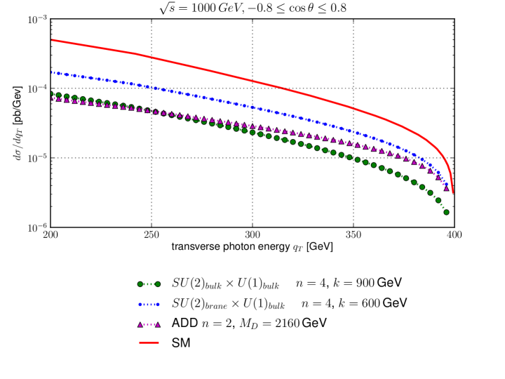
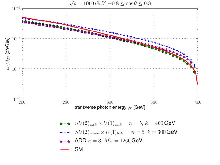
Figure 5:   

Differential $e^{+}e^{-}\rightarrow\gamma+\mbox{nothing}$ cross-section at $\sqrt{s}=1$TeV integrated over angle between photon and beam in the range $-0.8<\cos\theta<0.8$. We have imposed the cut $q<400$ GeV for both signal and background.

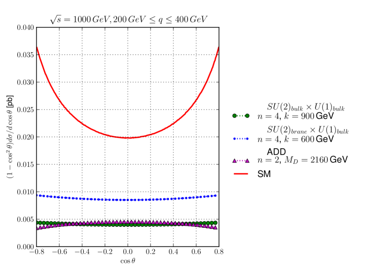
Figure 6:   

Differential $e^{+}e^{-}\rightarrow\gamma+$nothing cross-section at $e^{+}e^{-}$ collider at $\sqrt{s}=1$TeV integrated over photon momentum in the range $200$GeV$<q<400$GeV.

6 Conclusion

In this paper we have studied phenomenology of two Standard Model extensions in the modified Randall Sundrum II background metric. We found that the parameters of the models are constrained by the measurements of the invisible width of the $Z$ boson. We computed the cross-section of process $e^{+}e^{-}\rightarrow\gamma+nothing$ in these models, and found that the signal may be sizeable for $n\geq 5$.

An obvious extension of our analysis would be the study of the processes with missing energy in the final state at LHC, which are due to the vector bosons escaping from our brane. We hope to turn to this study in future.

We are indebted to V. A. Rubakov for helpful discussions and suggestions. We also thank S. N. Gninenko, D. S. Gorbunov, D. G. Levkov, M. V. Libanov, and E. Y. Nugaev for helpful discussions. This work was supported in part by the grant of the President of the Russian Federation NS-5525.2010.2, by the Ministry of Science and Education under state contracts 02.740.11.0244 and P2598, grant of the President of the Russian Federation MK-7748.2010.2.

References

• [1] V. A. Rubakov and M. E. Shaposhnikov, Phys. Lett.  B 125, 136 (1983). K. Akama, Lect. Notes Phys.  176, 267 (1982) [arXiv:hep-th/0001113].
• [2] S. L. Dubovsky, V. A. Rubakov and S. M. Sibiryakov, JHEP 0201, 037 (2002) [arXiv:hep-th/0201025].
• [3] L. Randall and R. Sundrum, Phys. Rev. Lett.  83, 4690 (1999) [arXiv:hep-th/9906064].
• [4] B. Bajc and G. Gabadadze, Phys. Lett.  B 474, 282 (2000) [arXiv:hep-th/9912232].
• [5] I. Oda, Phys. Lett.  B 496, 113 (2000) [arXiv:hep-th/0006203].
• [6] S. L. Dubovsky, V. A. Rubakov and P. G. Tinyakov, Phys. Rev.  D 62, 105011 (2000) [arXiv:hep-th/0006046].
• [7] S. L. Dubovsky, V. A. Rubakov and P. G. Tinyakov, JHEP 0008, 041 (2000) [arXiv:hep-ph/0007179].
• [8] R. Gregory, V. A. Rubakov and S. M. Sibiryakov, Class. Quant. Grav.  17, 4437 (2000) [arXiv:hep-th/0003109].
• [9] S. B. Giddings and E. Katz, J. Math. Phys.  42, 3082 (2001) [arXiv:hep-th/0009176].
• [10] R. Gregory, Phys. Rev. Lett.  84, 2564 (2000) [arXiv:hep-th/9911015].
• [11] T. Gherghetta and M. E. Shaposhnikov, Phys. Rev. Lett.  85, 240 (2000) [arXiv:hep-th/0004014].
• [12] S. L. Dubovsky and V. A. Rubakov, Int. J. Mod. Phys.  A 16, 4331 (2001) [arXiv:hep-th/0105243].
• [13] S. N. Gninenko, N. V. Krasnikov, and A. Rubbia, Phys. Rev. D 67, 075012 (2003)
• [14] A. Friedland and M. Giannotti, Phys. Rev. Lett. 100, 031602 (2008).
• [15] S. N. Gninenko, N. V. Krasnikov, and V. A. Matveev, Phys. Rev. D 78, 097701 (2008) [arXiv:0811.0974]
• [16] N. Arkani-Hamed, S. Dimopoulos and G. R. Dvali, Phys. Lett.  B 429, 263 (1998) [arXiv:hep-ph/9803315].
• [17] G. F. Giudice, R. Rattazzi and J. D. Wells, Nucl. Phys.  B 544, 3 (1999) [arXiv:hep-ph/9811291].
• [18] V. A. Rubakov, Phys. Usp.  44, 871 (2001) [Usp. Fiz. Nauk 171, 913 (2001)] [arXiv:hep-ph/0104152].
• [19] E. Boos, V. Bunichev, M. Dubinin, L. Dudko, V. Edneral, V. Ilyin, A. Kryukov, V. Savrin, A. Semenov, and A. Sherstnev PoS ACAT08:008, 2009 [arXiv:0901.4757].
• [20] C. Amsler et al. [Particle Data Group], Phys. Lett.  B 667, 1 (2008).