The solar photospheric abundance of zirconium

Abstract

Zirconium (Zr), together with strontium and yttrium, is an important element in the understanding of the Galactic nucleosynthesis. In fact, the triad Sr-Y-Zr constitutes the first peak of s-process elements. Despite its general relevance not many studies of the solar abundance of Zr were conducted. We derive the zirconium abundance in the solar photosphere with the same CO5BOLD hydrodynamical model of the solar atmosphere that we previously used to investigate the abundances of C-N-O. We review the zirconium lines available in the observed solar spectra and select a sample of lines to determine the zirconium abundance, considering lines of neutral and singly ionised zirconium. We apply different line profile fitting strategies for a reliable analysis of Zr lines that are blended by lines of other elements. The abundance obtained from lines of neutral zirconium is very uncertain because these lines are commonly blended and weak in the solar spectrum. However, we believe that some lines of ionised zirconium are reliable abundance indicators. Restricting the set to Zr ii lines, from the CO5BOLD 3D model atmosphere we derive A(Zr)=$2.62\pm 0.06$, where the quoted error is the RMS line-to-line scatter.

1 Introduction

The photospheric solar abundances of some elements have been studied more often than others; this is mainly due to the importance of the elements to explain nucleosynthesic processes. Moreover, the difficulty of extracting suitable lines with accurately known transition probabilities in the visible range of the solar spectrum can also explain why some elements have been studied less extensively.

For the triad Sr-Y-Zr, there exist only a few detailed studies of their solar abundances (an ADS search yields 4 papers for Sr, 5 for Y, and 10 for Zr) in spite of their importance in Galactic chemical evolution. Sr-Y-Zr, Ba-La, and Pb are located at three abundance peaks of the s-processes producing the enrichment of these elements in the Galaxy. Knowledge of the present Sr-Y-Zr abundances in stars of different metallicity and age is required to understand the complicated nucleosynthesis of these elements (for details see Travaglio et al. 2004).

Zirconium is present in the solar spectrum with lines of Zr i and Zr ii. The dominant species is Zr ii. According to our 3D model, and in agreement with our 1D reference model, about 99% of zirconium is singly ionised in the solar photosphere. Departure from local thermodynamical equilibrium (LTE) probably affects Zr i lines, producing a too low Zr abundance under the assumption of LTE. In fact NLTE effects, even on weak unsaturated Zr i lines, have been found by Brown et al. (1983) for G and K giants. However, both Biemont et al. (1981) and Bogdanovich et al. (1996) analysed in LTE Zr i lines (34 and 21 lines, respectively) and Zr ii lines (24 and 15 lines, respectively) in the solar photosphere, and found an excellent agreement between the abundances derived from both ionisation stages. Very recently Velichko et al. (2010) performed a NLTE analysis of zirconium in the case of the Sun and late type stars. According to their computations the NLTE abundance is larger than the LTE one, by up to 0.03 dex for Zr ii and by 0.29 dex for Zr i.

Owing to the small number of Zr i and Zr ii lines in metal poor stars (Gratton & Sneden 1994), it is important to analyse both of them in the solar photosphere to derive the solar abundance from both ionisation stages and to assess the agreement between the derived abundances. In spectra of cool stars it is easier to observe Zr i lines. For example, Goswami & Aoki (2010) realised that none of the Zr ii lines were usable in their analysis of the cool Pop. II CH star HD 209621, and the Zr abundance is derived from the only Zr i line in their spectrum at 613.457 nm. A similar situation had been encountered by Vanture & Wallerstein (2002) in their study of the Zr/Ti abundance ratio in cool S stars, where only Zr i lines in the red part of the spectrum can be used.

2 Lines and atomic data

According to Malcheva et al. (2006), zirconium has five stable isotopes. Four of them (⁹⁰Zr, ⁹¹Zr, ⁹²Zr, and ⁹⁴Zr) are produced by the s-process; the fifth, ⁹⁶Zr, is produced in the r-process. Zirconium is a very refractory element, it is difficult to be vaporised by conventional thermal means and, consequently, has been relatively little investigated in the laboratory.

In Table 1 and Table 2 the Zr i and Zr ii lines, with the $\log\,gf$ values available in the literature are collected.

Biemont et al. (1981) selected lines that lie at $\lambda$ $<$ 800 nm. They derived $\log\,gf$ using the technique developed by Hannaford & Lowe (1981), suitable for highly refractory elements like Zr, to determine lifetimes of 34 levels of Zr i and 20 levels of Zr ii. From these measurements, coupled with the measurements of branching ratios, they derived the $\log\,gf$ values of 38 Zr i and 31 Zr ii lines.

Bogdanovich et al. (1996) computed and used $\log\,gf$ values for 21 Zr i lines. They give new $\log\,gf$ values for 15 Zr ii lines among those selected by Biemont et al. (1981). Their $\log\,gf$ are given in Table 2.

Sikström et al. (1999) derived the abundance of zirconium in HgMn star $\chi$ Lupi, finding a disagreement when using Zr ii or Zr iii lines. They measured the f-values for several Zr ii lines in the UV at $\lambda<300$ nm.

Vanture & Wallerstein (2002) extended the search for Zr i lines in the near-IR, at wavelengths longer than 800 nm, a region important in the study of cool stars, because this is the region were cool stars emit most of their flux. The complete sample of these near-infrared lines is also given in Table 1. Because absorption bands of molecules are weak in the warmer S stars, these near-IR zirconium lines are better abundance indicators than the Zr ii lines in the blue part of the spectrum. These lines are, however, not necessarily good for the Sun.

We have also checked the 13 Zr i lines identified by Swensson et al. (1970) in the Delbouille et al. (1981) atlas, but 12 of them appear severely blended. Only the line at 784.9 nm is retained in Table 1, as it was by Biemont et al. (1981) and Vanture & Wallerstein (2002).

In the present analysis we adopt the $\log\,gf$ values of Biemont et al. (1981) for all Zr i lines.

According to the NIST database, Zr ii lines lie only in the near UV-blue (241.941-535.035 nm); only two weak lines (at 667.801 and 678.715 nm) are present in NIST with $\lambda>$540 nm.

The line identifications by Moore et al. (1966) on the Utrecht solar atlas have been used by Biemont et al. (1981) to select 31 Zr ii lines, seven of which were later discarded because the derived abundance exceeded the mean by more than 3$\sigma$, so they are likely blended with other unknown species. Gratton & Sneden (1994) used the same line list as Biemont et al. (1981). Ljung et al. (2006) derived new oscillator strengths for 263 Zr ii lines and studied 7 lines, the lines that they judged to be the best and unperturbed in the photospheric spectrum, to derive the solar Zr abundance based on both 1D and 3D model atmospheres.

We extracted from the 243 lines by Malcheva et al. (2006), those in common with Biemont et al. (1981); for these lines the best values of $\log\,gf$, according to Malcheva et al. (2006), are the same as in Biemont et al. (1981). We compared the new $\log\,gf$ values determined by Ljung et al. (2006) with those by Biemont et al. (1981). There is a good agreement for most of the lines, with a few exceptions (see Table 2). We report all these values in Table 2.

In the present analysis we used the $\log\,gf$ values of Ljung et al. (2006) for all the Zr ii lines.

Table 1: Lines of Zr i chosen by Biemont et al. (1981) and Vanture & Wallerstein (2002)

$\lambda$	Elow	EW	$\log\,gf$
nm	eV	pm	B	VW	Bog
350.9331	0.07	0.65	–0.11		–0.21
360.1198	0.15	1.3	–0.47
389.1383	0.15	1.7	–0.10
402.893	0.52	0.06	–0.72
403.0049	0.60	0.26	–0.36		–0.59
404.3609	0.52	0.58	–0.37
407.2696	0.69	0.57	+0.31		+0.24
424.1706	0.65	0.37	+0.14		+0.07
450.7100	0.54	0.36	–0.43		–0.46
454.2234	0.63	0.46	–0.31
468.7805	0.73	1.00	+0.55		+0.30
471.0077	0.69	1.05	+0.37		+0.19
473.2323	0.63	0.25	–0.49		–0.56
473.9454	0.65	0.55	+0.23		+0.07
477.2310	0.62	0.53	+0.04		–0.07
478.494	0.69	0.16	–0.49
480.589	0.69	0.15	–0.42		–0.63
480.9477	1.58	0.16	+0.16
481.5056	0.65	0.20	–0.53		–0.22
481.5637	0.60	0.30	–0.03
482.806	0.62	0.19	–0.64
504.655	1.53	0.050	+0.06		–0.25
538.5128	0.52	0.18	–0.71
612.746	0.15	0.21	–1.06	–1.06	–0.87
613.457	0.00	0.19	–1.28	–1.28	–1.05
614.046	0.52	0.073	–1.41	–1.41	–0.85
614.3183	0.07	0.21	–1.10	–1.10	–0.98
631.303	1.58	0.11	+0.27		+0.18
644.572	1.00	0.094	–0.83	–0.83
699.084	0.62	0.050	–1.22		–1.44
709.776	0.69	0.21	–0.57
710.289	0.65	0.065	–0.84		–1.06
743.989	0.54			–1.18
755.149	1.58			–1.36
755.473	0.51			–2.28
755.841	1.54			–1.47
756.213	0.62			–2.71
781.935	1.82	0.065	–0.38	–0.39
782.292	1.75			–1.14
784.938	0.69	0.10	–1.30	–1.30
856.859	0.73			–2.80
857.1085	1.53			–2.07
858.421	1.86			–1.32
858.787	1.48			–2.12
874.958	0.60			–2.79
350.1133	0.07	0.7	–0.93
357.5765	0.07	3.3	–0.03
366.3698	0.15	2.5	+0.01
588.5629	0.07	0.050	–2.12		-1.82

B: Biemont et al. (1981)
VW: Vanture & Wallerstein (2002)
Bog: Bogdanovich et al. (1996)

Table 2: Lines of Zr ii chosen by Biemont et al. (1981) and Ljung et al. (2006)

$\lambda$	Elow	EW [pm]		$\log\,gf$
nm	eV	B	L	B	Bog	L
343.2415	0.93	2.1		–0.75	–0.51	–0.72
345.4572	0.93	1.00		–1.34		–1.33
345.8940	0.96	1.6		–0.52		–0.48
347.9017	0.53	2.8		–0.69	–1.12	–0.67
347.9393	0.71	5.1		+0.17	+0.12	+0.18
349.9571	0.41	2.4		–0.81	–1.08	–1.06
350.5666	0.16	5.1		–0.36	–0.62	–0.39
354.9508	1.24	1.6		–0.40	–0.68	–0.72
355.1951	0.09	5.8		–0.31		–0.36
358.8325	0.41	2.7		–1.13	–1.25	–1.13
360.7369	1.24	1.3		–0.64	–0.48	–0.70
367.1264	0.71	3.2		–0.60	–0.56	–0.58
371.4777	0.53	3.0		–0.93		–0.96
379.6496	1.01	1.5		–0.83	–1.17	–0.89
383.6769	0.56	4.7		–0.06	–0.22	–0.12
403.4091	0.80	0.65		–1.55		–1.51
405.0320	0.71	2.38	2.20	–1.00	–0.60	–1.06
408.5719	0.93	0.54		–1.61	–1.54	–1.84
420.8980	0.71	4.3	4.26	–0.46		–0.51
425.8041	0.56	2.6	2.34	–1.13		–1.20
431.7321	0.71	1.20		–1.38		–1.45
444.2992	1.49	2.0	2.04	–0.33		–0.42
449.6962	0.71	3.6	3.15	–0.81	–0.87	–0.89
511.2270	1.66	0.83	0.78	–0.59	–0.58	–0.85
363.0027	0.36	3.8		–1.11		–1.11
407.1093	1.00	2.1		–1.60		–1.66
414.9202	0.80	7.5		–0.03		–0.04
416.1208	0.71	5.8		–0.72		–0.59
426.4925	1.66	1.50		–1.41		–1.63
444.5849	1.66	0.83		–1.35
461.3921	0.97	2.91		–1.52		–1.54
402.4435	0.999		1.20			–1.13

B: Biemont et al. (1981)
Bog: Bogdanovich et al. (1996)
L: Ljung et al. (2006)

3 Solar Zr abundance in the literature

Several analyses of the solar Zr abundance, made before 1980, used Corliss & Bozman (1962) $\log\,gf$ (Aller 1965, Wallerstein 1966, Grevesse et al. 1968) or older ones (Goldberg et al. 1960) or have been made to derive a temperature correction for the Corliss & Bozman (1962) data (Allen 1976). The use of these transition probabilities, which are known to contain errors depending on excitation and temperature, coupled with the use of old solar spectral atlases, explains discrepancies of these Zr abundance determinations based either on Zr i and/or Zr ii.

We concentrate on the more recent determinations of the photospheric solar Zr abundance, that we summarise below.

1. Biemont et al. (1981) analysed the Delbouille et al. (1973) atlas. The equivalent widths (EWs) were independently measured by E. Bièmont and N. Grevesse, and the results examined and discussed to produce the final list. They used the Holweger-Müller solar model (Holweger 1967; Holweger & Müller 1974) with a microturbulence, $\xi$, of $0.8$ $\mathrm{km\,s^{-1}}$. They note that their analysis is independent of line-broadening parameters since most of the lines are faint or very faint. The $\log\,gf$ are from their own measurements. They find that the abundance from Zr i lines is independent of $\xi$ and that the abundance from Zr ii lines is insensitive to the model. These authors rejected 4 Zr i lines and 7 Zr ii lines from their selected sample in their final solar abundance analysis because they imply a Zr abundance which is more than 3$\sigma$ higher than the average. These lines appear after the horizontal line in Tables 1 and 2. They conclude that Zr ii lines are better abundance indicators. They obtain a zirconium abundance of A(Zr)=$2.57\pm 0.07$ from Zr i (34 lines) and A(Zr)=$2.56\pm 0.07$ from Zr ii (24 lines).

2. Gratton & Sneden (1994) studied the Zr behaviour in metal-poor stars. They used as model atmosphere a grid from Bell et al. (1976) for giants, and a similar grid for dwarfs provided by Bell. They also analysed the solar spectrum, to have a reference A(Zr)$\odot$. For this purpose they used the same 24 lines as Biemont et al. (1981), the Holweger-Müller model with microturbulence of $1.5$ $\mathrm{km\,s^{-1}}$, and the solar abundances from Anders & Grevesse (1989). They remark that in their metal poor stars Zr abundances from Zr i are, on average, lower than those from Zr ii lines, a result similar to that found by Brown et al. (1983) for Pop. I stars. For the analysis of the metal poor stars they used 7 Zr ii lines and 3 of them (407.1, 414.9, and 416.1 nm) are among those discarded by Biemont et al. (1981), suggesting that these are no longer significantly blended in metal poor stars. They obtain for the solar Zr abundance 2.59$\pm$0.04 from Zr i (34 lines) $\sigma$=0.22 dex, 2.53$\pm$0.03 from Zr ii (24 lines) $\sigma$=0.14 dex, respectively.

3. Bogdanovich et al. (1996) computed theoretical $\log\,gf$, and used the Holweger-Müller model with $\xi$=0.8, and a model computed with a code by Kipper et al. (1981) which is a modified version of the ATLAS 5 code (Kurucz 1970). They used the damping constants modified by Galdikas (1988), and the EW measurements of Biemont et al. (1981). The results are: A(Zr)=2.60$\pm$0.07 from Zr i (21 lines) and A(Zr)=2.61$\pm$0.11 from Zr ii (15 lines). They adopted A(Zr)$=2.60\pm 0.06$.

4. Ljung et al. (2006) considered only Zr ii lines, they used $\log\,gf$ from experimental branching ratios measured by them, and radiative lifetimes taken from different papers. They used 1D Holweger-Müller and MARCS models, and a 3D model computed with the Stein-Nordlund code (Stein & Nordlund 1998) for line profile fitting. EWs of the best 3D fitting profiles are used to estimate the abundance. From 7 Zr ii lines, six of which in common with Biemont et al. (1981), they obtain A(Zr)=$2.58\pm 0.02$ with the 3D model, A(Zr)=$2.56\pm 0.02$ with MARCS model, and A(Zr)=$2.63\pm 0.02$ with the HM model. Their adopted value is A(Zr)=$2.58\pm 0.02$.

5. Velichko et al. (2010) performed the first NLTE analysis of Zr in the solar photosphere. They investigated all the Zr lines analysed by Biemont et al. (1981) and Ljung et al. (2006) and selected a subsample of two Zr i lines (424.1 and 468.7 nm) and ten Zr ii lines (347.9, 350.5, 355.1, 405.0, 420.8, 425.8, 444.2, 449.6, and 511.2 nm). Analysing the Kurucz (2005a) solar spectrum with a MAFAGS model atmosphere (5780 K/4.44/0.0) and a microturbulence of 0.9$\mathrm{km\,s^{-1}}$they derive a LTE abundance of 2.33 and 2.61 from Zr i and Zr ii lines, respectively. They constructed a Zr model atom and derived the NLTE abundance with different assumptions about the rates of collisions with H-atoms. In their scenario, the NLTE abundance is always higher than the LTE abundance varying in a range from 0.21 to 0.32 dex for Zr i and from 0.01 to 0.08 dex for Zr ii, depending on the adopted cross sections for collision with H-atoms. Their best estimate of the NLTE abundance (correction) from Zr i and Zr ii lines is 2.62 (0.29) and 2.64 (0.03) dex, respectively. Their adopted Zr abundance is $2.63\pm 0.07$.

The abundance of Zr in the solar system is derived from the analysis of meteorites. Zirconium is not a volatile element, and its abundance in meteorites should agree with the one in the solar photosphere. To compare the abundances derived from the meteorites, on the cosmochemical abundance scale relative to $10^{6}$ Si atoms, with the ones derived form the solar photosphere, on the astronomical scale of $10^{12}$ H-atoms, a coupling factor must be derived. Lodders (2003) and Lodders et al. (2009) to link the two scales introduce an average factor by looking at a sample of refractory elements well-determined in the photosphere and at the same elements in meteorites. In this way the factor is not affected by the individual uncertainty and, if the abundance of one element derived from the photosphere changes, the conversion factor is not much affected.

The meteoritic Zr abundance is A(Zr)=$2.57\pm 0.04$, Lodders et al. (2009). Other Zr meteoritic values that can be found in the literature are: $2.61\pm 0.03$ according to Anders & Grevesse (1989), $2.61\pm 0.02$ according to Grevesse & Sauval (1998), $2.60\pm 0.02$ according to Lodders (2003). The value of $2.53\pm 0.04$ given in Asplund et al. (2009) is based on the same data from Lodders et al. (2009), but they give a lower value for Zr on the astronomical scale because they use a lower coupling factor for the cosmochemical and astronomical scales. In the same way the value of $2.57\pm 0.02$ in Asplund et al. (2005) and Grevesse et al. (2007) is based on data from Lodders (2003), but their value is lower because again a different scaling factor (which is 0.03 $\log$ units smaller than the one recommended in Lodders (2003)) was used.

4 Model atmospheres

We base our abundance analysis on the same model atmospheres that we used in the previous analysis of solar abundance determinations, summarised in Caffau et al. (2010). We rely on a time-dependent, 3D hydrodynamical model atmosphere, computed with the CO⁵BOLD code; see Freytag, Steffen, & Dorch (2002) and Freytag et al. (2010) for details. This model has a box size of $5.6\times 5.6\times 2.27\,{\rm Mm}^{3}$, resolved by $140\times 140\times 150$ grid points. Its range in Rosseland optical depth is $-6.7<\log\tau_{\rm Ross}<5.5$. The complete time series is formed by 90 snapshots covering 1.2 h of solar time. For the spectral synthesis computations we selected 19 representative snapshots out of the complete series of 90 snapshots.

To compute 3D-corrections for the zirconium abundance, we make use of two 1D reference atmospheres: the 1D model obtained by horizontally averaging each 3D snapshot over surfaces of equal (Rosseland) optical depth (henceforth $\left\langle\mathrm{3D}\right\rangle$ model), and the hydrostatic 1D mixing-length model computed with the LHD code, that employs the same micro-physics and radiative transfer scheme as the CO⁵BOLD code, (henceforth $\mathrm{1D}_{\mathrm{LHD}}$ model). We define 3D-corrections as in Caffau et al. (2010), ${\Delta_{\rm gran}={\rm A(Zr)}_{\rm 3D}}-{\rm A(Zr)}_{\rm\left\langle\mathrm{3D}\right\rangle}$, to isolate the effects of horizontal fluctuations (granulation effects), and ${\Delta_{\rm LHD}={\rm A(Zr)}_{\rm 3D}}-{\rm A(Zr)}_{\rm LHD}$, to measure the total 3D effect. For details see Caffau et al. (2010) and Caffau & Ludwig (2007).

We also considered the semi-empirical Holweger-Müller solar model (Holweger 1967; Holweger & Müller 1974, hereafter HM) for comparison.

5 Observed spectra

We analysed the same four solar spectral atlases, publicly available (two disc-centre and two disc-integrated atlases), that we used in all our previous works on solar abundances, such as in Caffau et al. (2010). These high resolution, high signal-to-noise ratio (S/N) spectra, are:

1. the disc-integrated spectrum of Kurucz (2005a), based on fifty solar FTS scans, observed by J. Brault and L. Testerman at Kitt Peak between 1981 and 1984;

2. the FTS atlas of Neckel & Labs (1984), observed at Kitt Peak in the 1980ies, providing both disc-centre and disc-integrated data;

3. the disc-centre atlas of Delbouille et al. (1973), observed from the Jungfraujoch.

6 Abundance determination methods

In principle, the best way to derive the abundance of an element from a spectral line is by line profile fitting. Once the atomic data are known, this technique allows to take into account the strength of the line and its shape at the same time. The limiting factor is that the observed solar spectra are of such a good quality that the synthetic line profile is often not realistic enough to reproduce the shape of the line in the observed spectrum. Synthetic line profiles derived from 1D model atmospheres do not take into account the line asymmetry induced by convection, they are symmetric. In many cases NLTE effects modify the line profile (see Asplund et al. 2004). In case the line is not clean, but some contaminating lines are present in the range, the line profile fitting should take into account these blending components. Good atomic data for these blending lines are then necessary, and, as for the line of interest, granulation and NLTE effects can be limiting factors.

To fit a line blended with other components, one has to optimise the agreement between synthetic and observed spectra also for the blending lines, allowing, in the line profile fitting process, the abundance of the blending lines to change as well. Even though the 3D spectrum synthesis is still computationally demanding, we have attempted to derive A(Zr) by properly taking into account also the blending lines whenever possible. In the fitting procedure, the Zr abundance and the abundances of the blending lines are adjusted independently until the best match of the observed spectrum is achieved (in the following referred to as method ‘A’).

We also tested a simplified fitting approach (in the following method ’B’): we synthesised one typical 3D profile of each blending components, in addition to a grid with different abundances for the Zr line of interest. Then, in the fitting procedure, a profile is interpolated in the grid for Zr, while the profiles (more precisely the relative line depressions) of the blending lines are simply scaled, and then the blending lines and the Zr line are added linearly to obtain the composite line profile. In the fitting procedure, the Zr abundance and the scaling factors (and shifts) of the blending lines are adjusted until the best agreement with the observed spectrum is found. An advantage of this fitting procedure is that it works even if the atomic data of the blending components are poorly known. Note, however, that this procedure is theoretically justified only if all the lines are on the linear part of the curve of growth. If the lines are partly saturated, the line strengths of all components are underestimated, and so is the derived Zr abundance. Nevertheless, method ’B’ was also applied to partly saturated lines in order to understand its limitations.

Methods ’A’ and ’B’ provide the Zr abundance without the need to measure an equivalent width. However, we can formally derive the equivalent width of the Zr component from the synthetic line profile computed for Zr only (ignoring all blends) with the Zr abundance that provides the best fit of the observed spectrum. For method ’B’, this is simply the equivalent width of the Zr line that gives the best agreement between added-synthetic and observed profile.

A third alternative (method ’C’) is the measurement of the equivalent width of the line of interest, which is then translated into an abundance via the 3D curve-of-growth. For this purpose, we employ the IRAF task splot for fitting Gaussian or Voigt profiles to the observed line. Even in the case that the line of interest is contaminated by unidentified components, which cannot be taken into account with methods ’A’ and ’B’, it may still be possible to use splot with the deblending option to determine the equivalent widths of all components. This procedure may also be useful if the number of blending lines is too large to be treated conveniently by the methods ’A’ or ’B’ based on synthetic spectra. However, as method ’B’, this approach is only justified if all involved lines are weak.

7 Zirconium abundance from Zr i lines

We looked at the Zr i lines in the sample of Biemont et al. (1981). All these lines are rather weak and blended, or in a crowded spectral region. After inspection, we analysed a subsample of 11 lines, discarding the lines we think to be too heavily blended and/or in a too crowded range. We found our EW measurements to be affected by rather large uncertainties, but for the majority of the 11 lines we agree with the results of Biemont et al. (1981). We think that the cleanest lines are the ones at 480.9, 481.50, 614.0, and 644.5 nm, but also these lines are too poor to give precise information on the solar abundance. We found it difficult to use the flux spectra to measure the EWs of so weak and blended lines, and decided to use only the disc-centre spectra, which are sharper. From the four clean lines mentioned above, we obtain, A(Zr)$=2.65\pm 0.07$. If we remove also the 644.5 pm line we obtain A(Zr)$=2.62\pm 0.04$. This result is in perfect agreement with the abundance obtained from Zr ii lines (see below), but we consider this agreement fortuitous. From the $\mathrm{1D}_{\mathrm{LHD}}$ model we find a slightly higher value of A(Zr)=$2.67\pm 0.07$, and from the $\left\langle\mathrm{3D}\right\rangle$ model A(Zr)=$2.74\pm 0.08$.

8 Investigation of Zr ii lines

We picked up all the Zr ii lines of Biemont et al. (1981) and the line at 402.4 pm analysed in Ljung et al. (2006). Our starting sample was formed by 32 Zr ii lines. After inspection of the observed data, and comparison with 1D synthetic spectra, we discarded 11 lines that we think are too heavily blended. After analysis, we discarded four other lines that also Biemont et al. (1981) rejected because they provided a too high abundance. Our final sample is formed by the seven lines of Ljung et al. (2006), that we discuss one by one in the next section, and 10 lines that are used for the abundance analysis in Biemont et al. (1981).

These Zr ii lines have lower level energies below 1.7 eV. If we look at the equivalent width contribution functions for disc-centre of the 3D model, we can see that they are formed in a range in $\tau_{\rm Ross}$ between $-4$ and $0$, with the maximum in the range $-1.0<\tau_{\rm Ross}<-0.5$ (see Fig. 1). Only two lines (350.5 and 355.1 nm) are formed over a larger range, with a maximum around $\tau_{\rm Ross}\approx-2.0$, because these two lines have smaller lower level energies, and are significantly stronger than the others.

Figure 1: Temporal and horizontal average of the temperature profile of the 3D model (solid line) and the temperature profile of $\mathrm{1D}_{\mathrm{LHD}}$ model, shown as a function of (Rosseland) optical depth. In addition, the equivalent width contribution functions (lower, roughly Gaussian-shaped curves) for the 405.0 nm Zr ii line are plotted on the same optical depth scale for disc-centre (solid line) and disc-integrated spectra (dashed line).

The abundance results we obtained from the Zr ii lines are summarised in Table 3. We averaged the EW measured in the two disc-centre and the two disc-integrated spectra, respectively. The last column of the table indicates if the result refers to disc-centre or disc-integrated spectra. From the complete sample of 17 lines we obtain A(Zr)=2.612$\pm$0.093, with $2.638\pm 0.078$ and $2.586\pm 0.100$ from disc-centre and disc-integrated spectra, respectively. The line at 347.9 nm gives a very low abundance, while the line at 355.1 nm gives a rather high one. Both these two lines lie in a very crowded region of the spectrum and it is very difficult to place the continuum. When we remove these two lines from the sample, we have 15 Zr ii lines and we obtain A(Zr)=2.616$\pm$0.060, with $2.643\pm 0.050$ and $2.589\pm 0.057$ from disc-centre and disc-integrated spectra, respectively. We note that the 3D abundance from flux is systematically lower than the one from the intensity spectra.

When we look only at the seven lines from Ljung et al. (2006), we find that the line-to-line scatter is reduced with respect to the sample of 15 lines. The 3D abundance we find is $2.653\pm 0.022$ and $2.623\pm 0.031$ for disc-centre and disc-integrated data, respectively. The abundance averaged over both disc-centre and disc-integrated spectra is $2.638\pm 0.031$. We find a very low line-to-line scatter, but again the disc-centre spectra give a systematically higher abundance than the disc-integrated spectra, by an amount comparable to the line-to-line scatter of $\approx 0.03$ dex.

We found similar results for Fe, Hf, and Th, where the abundances derived from disc-integrated spectra are lower by 0.02, 0.05, and 0.02 dex, respectively, than the disc-centre abundances (see Caffau et al. 2008 and Caffau et al. 2010 for details). A similar behaviour is seen when using 1D model atmospheres. We have presently no obvious explanation for this result.

The zirconium abundance derived from 1D models depends on the choice of the microturbulence parameter $\xi$. The microturbulence we find for the sample of 15 Zr ii lines, by requiring that the relation between EW and A(Zr) obtained with the 1D model has the same slope as that of the 3D model (method 3a in Steffen et al. (2009)), is consistent with the results obtained by Steffen et al. (2009) from a sample of Fe ii lines. We adopt $\xi=1.0$ $\mathrm{km\,s^{-1}}$ for the analysis of disc-integrated spectra, and obtain A(Zr)${}_{\left\langle\mathrm{3D}\right\rangle}=2.597\pm 0.053$ and A(Zr)${}_{\rm LHD}=2.575\pm 0.057$. For disc-centre data, we choose $\xi=0.7$ $\mathrm{km\,s^{-1}}$ and the result is A(Zr)${}_{\left\langle\mathrm{3D}\right\rangle}=2.652\pm 0.044$ and A(Zr)${}_{\rm LHD}=2.635\pm 0.045$ (for $\xi=1.0$ $\mathrm{km\,s^{-1}}$ we get A(Zr)${}_{\left\langle\mathrm{3D}\right\rangle}=2.602\pm 0.067$, A(Zr)${}_{\rm LHD}=2.587\pm 0.072$).

3D corrections are small in absolute value and depend on the value of the microturbulence. The average 3D correction with respect to the reference $\mathrm{1D}_{\mathrm{LHD}}$ model is positive, $\Delta_{\rm LHD}=+0.011\pm 0.012$ dex, while, with respect to the $\left\langle\mathrm{3D}\right\rangle$ model it is slightly negative, $\Delta_{\rm gran}=-0.008\pm 0.016$ dex, again taking $\xi=0.7$ $\mathrm{km\,s^{-1}}$ for disc-centre and $\xi=1.0$ $\mathrm{km\,s^{-1}}$ for disc-integrated spectra.

With the HM model we obtain A(Zr)${}_{\rm HM}=2.679\pm 0.044$ and A(Zr)${}_{\rm HM}=2.619\pm 0.053$ for disc-centre and integrated disc, respectively. Taking into account both lines of disc-centre and integrated disc, we obtain A(Zr)${}_{\rm HM}=2.649\pm 0.057$, and when applying the $\Delta_{\rm gran}$ correction, we have A(Zr)${}_{\rm HM}=2.641\pm 0.057$.

For our final determination of the solar zirconium abundance, we adopt the complete sample of 15 Zr ii lines, and our recommended value is A(Zr)${}_{\rm 3D}=2.62\pm 0.06$, obtained with 3D model atmosphere.

Table 3: The results from the 7 lines of Zr ii from Ljung et al. (2006), and other 10 lines from Biemont et al. (1981).

$\lambda$	Elow	EW	$\log\,gf$	A(Zr)				3D-Corrections		Sp
nm	eV	pm		3D	$\left\langle\mathrm{3D}\right\rangle$	$\mathrm{1D}_{\mathrm{LHD}}$	HM	$\Delta_{\rm gran}$	$\Delta_{\rm LHD}$
					$\xi=1.0/0.7$ $\mathrm{km\,s^{-1}}$			$\xi=1.0/0.7$ $\mathrm{km\,s^{-1}}$
402.4453	0.999	1.33	–1.13	2.667	2.645/2.660	2.640/2.655	2.673/2.689	0.022/ 0.007	0.027/ 0.012	I
402.4453	0.999	1.43	–1.13	2.613	2.616/2.636	2.602/2.622	2.638/2.659	–0.003/–0.023	0.011/–0.009	F
405.0320	0.713	2.17	–1.06	2.617	2.588/2.620	2.577/2.608	2.617/2.649	0.029/–0.003	0.040/ 0.009	I
405.0320	0.713	2.40	–1.06	2.583	2.593/2.637	2.573/2.615	2.617/2.662	–0.010/–0.054	0.010/–0.032	F
420.8980	0.713	4.22	–0.51	2.630	2.559/2.671	2.533/2.640	2.592/2.707	0.071/–0.040	0.098/–0.010	I
420.8980	0.713	4.45	–0.51	2.578	2.596/2.733	2.561/2.693	2.627/2.767	–0.018/–0.155	0.017/–0.116	F
425.8041	0.559	2.36	–1.20	2.642	2.613/2.648	2.597/2.631	2.641/2.677	0.029/–0.006	0.045/ 0.011	I
425.8041	0.559	2.67	–1.20	2.627	2.640/2.691	2.616/2.665	2.664/2.716	–0.013/–0.064	0.011/–0.037	F
444.2992	1.486	2.19	–0.42	2.672	2.637/2.668	2.625/2.655	2.665/2.697	0.035/ 0.004	0.047/ 0.017	I
444.2992	1.486	2.38	–0.42	2.651	2.651/2.694	2.631/2.671	2.673/2.717	–0.000/–0.043	0.020/–0.020	F
449.6962	0.713	3.11	–0.89	2.661	2.618/2.674	2.596/2.649	2.647/2.704	0.042/–0.014	0.065/ 0.012	I
449.6962	0.713	3.41	–0.89	2.642	2.655/2.733	2.626/2.699	2.680/2.761	–0.013/–0.091	0.016/–0.057	F
511.2270	1.665	0.84	–0.85	2.685	2.664/2.672	2.653/2.661	2.688/2.697	0.021/ 0.013	0.032/ 0.024	I
511.2270	1.665	0.92	–0.85	2.666	2.662/2.673	2.647/2.658	2.679/2.691	0.004/–0.007	0.019/ 0.008	F
345.4572	0.931	0.96	–1.33	2.781	2.760/2.772	2.748/2.760	2.779/2.791	0.021/ 0.009	0.032/ 0.021	I
345.4572	0.931	1.00	–1.33	2.687	2.687/2.702	2.672/2.686	2.702/2.717	–0.001/–0.016	0.015/ 0.000	F
347.9017	0.527	2.80	–0.67	2.422	2.373/2.437	2.350/2.411	2.393/2.458	0.049/–0.015	0.072/ 0.011	I
347.9017	0.527	2.90	–0.67	2.315	2.330/2.406	2.301/2.375	2.348/2.424	–0.015/–0.091	0.014/–0.059	F
349.9571	0.409	2.50	–1.06	2.598	2.559/2.609	2.536/2.585	2.579/2.630	0.040/–0.011	0.062/ 0.014	I
349.9571	0.409	2.70	–1.06	2.525	2.540/2.606	2.513/2.576	2.558/2.624	–0.015/–0.081	0.012/–0.051	F
350.5666	0.164	5.10	–0.39	2.614	2.469/2.676	2.429/2.633	2.496/2.703	0.145/–0.062	0.185/–0.019	I
350.5666	0.164	5.40	–0.39	2.514	2.527/2.745	2.482/2.697	2.553/2.771	–0.013/–0.231	0.032/–0.183	F
354.9508	1.236	1.40	–0.72	2.656	2.627/2.646	2.613/2.632	2.645/2.665	0.029/ 0.009	0.042/ 0.023	I
354.9508	1.236	1.50	–0.72	2.585	2.585/2.611	2.567/2.591	2.599/2.625	0.000/–0.025	0.018/–0.006	F
355.1951	0.095	5.80	–0.36	2.773	2.604/2.826	2.561/2.781	2.632/2.853	0.169/–0.054	0.212/–0.008	I
355.1951	0.095	6.50	–0.36	2.806	2.795/3.012	2.746/2.958	2.823/3.037	0.011/–0.206	0.060/–0.152	F
360.7369	1.236	1.30	–0.70	2.587	2.560/2.577	2.546/2.563	2.578/2.596	0.028/ 0.010	0.041/ 0.024	I
360.7369	1.236	1.40	–0.70	2.520	2.519/2.542	2.501/2.523	2.533/2.556	0.001/–0.022	0.019/–0.003	F
367.1264	0.713	3.40	–0.58	2.555	2.505/2.587	2.493/2.573	2.538/2.623	0.051/–0.032	0.062/–0.017	I
367.1264	0.713	3.60	–0.58	2.493	2.513/2.616	2.489/2.588	2.542/2.648	–0.019/–0.123	0.005/–0.095	F
371.4777	0.527	3.00	–0.96	2.633	2.593/2.656	2.582/2.642	2.625/2.689	0.040/–0.022	0.051/–0.009	I
371.4777	0.527	3.20	–0.96	2.572	2.591/2.671	2.569/2.646	2.618/2.700	–0.019/–0.099	0.003/–0.073	F
408.5719	0.931	0.35	–1.84	2.652	2.637/2.640	2.635/2.638	2.664/2.668	0.015/ 0.011	0.017/ 0.014	I
408.5719	0.931	0.37	–1.84	2.582	2.581/2.586	2.571/2.575	2.602/2.606	0.001/–0.003	0.011/ 0.007	F

9 Analysis of a selected subsample of Zr ii lines

We particularly investigated the Zr ii lines selected by Ljung et al. (2006) for the solar abundance determination. We find this sample interesting because it contains: two mostly clean lines ($\lambda$  405.0, 420.8 nm), a line blended on the blue side ($\lambda$  449.6 nm), two lines blended on the red side ($\lambda$  402.4, 425.8 nm), and two lines blended on both sides ($\lambda$  444.2, 511.2 nm)

9.1 The Zr ii line at 402.4 nm

This weak Zr ii line is on the blue wing of a strong blend of Ti i and Fe ii where the Ti i line is the dominant component. On the blue wing of this Ti-Fe blend, there is also a Ce ii line. Close by, on the red side of the Ti i line, there is a strong line of iron blended with a much weaker Nd ii line. The zirconium abundance is determined with method ’B’ (see Sect. 6): to take into account the effects of the lines present in the range of the Zr ii line, we computed a 3D profile for each of the Ce ii line at 402.44, the Ti i line at 402.45 nm, and the strong Fe i line at 402.47 nm, to be used in the fitting process. The comparison of the best fitting 3D synthetic profile and the observed Delbouille et al. (1973) disc-centre spectrum is shown in Fig. 2. The Zr abundances and EWs resulting from the best fit of the four observed spectra are listed in Table 3.

The situation of the $402.4$ nm line may be compared to that of the 425.8 nm Zr ii line (see Sect. 9.4), and the $444.2$ nm Zr ii line (see Sect 9.5), for which we show below that the abundance is underestimated by about 0.03 dex and 0.01 dex, respectively, when using the approximate method ’B’.

The use of splot for the EW measurements is difficult in this case, also with the deblending option. In fact, several lines should be introduced in the range, making the profile fitting unstable.

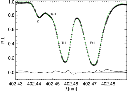
Figure 2: The observed solar disc-centre spectrum of Delbouille et al. (1973) in the region of the Zr ii line at 402.4 nm (black symbols), superimposed on the best fitting 3D synthetic profile obtained with method ’B’ (solid green/grey). The graph near the bottom shows the synthetic–observed residuals. The Zr abundance derived from this fit is A(Zr)=$2.602$.

We also fitted the line profile with a grid of 3D synthetic spectra computed with zirconium only. We limited the fitting to the blue wing and the line core, neglecting the red wing, which is blended with the other lines (see Fig. 3). In this kind of fit, neglecting the contribution of the other lines, the continuum placement, when considered as a free parameter, is problematic. When fixing the continuum, the abundance from the fit is in close agreement with the abundance determination from method ’B’, in the case of the disc-centre spectra within 0.03 dex (cf.  Fig. 3). For the disc-integrated spectra we find the fit to be ambiguous. The abundance comes out larger than from method ’B’ by about 0.1 dex, but the fit is convincing only when taking the atlas of Neckel & Labs (1984), although even in this case the core of the line is not well fitted. We find a different result from the two disc-integrated and the two disc-centre spectra, respectively, that we cannot easily explain. Maybe the differences are related to the fact that lines in flux spectra are more broadened than at disc-centre.

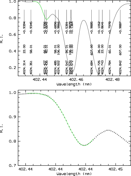
Figure 3: In the top panel, the observed solar disc-centre spectrum of Delbouille et al. (1973) in the region of the Zr ii line at 402.4 pm (black symbols), superimposed on the best fitting 3D synthetic profile (solid green/grey) obtained with a grid computed with only zirconium. In this fit A(Zr)=2.644. From the fit of the Neckel & Labs (1984) disc-centre profile, we get A(Zr)=2.669. The lower panel shows a zoom in the fitting range.

9.2 The Zr ii line at 405.0 nm

This line seems to be unblended. A weaker line is on the red side at about $\Delta\lambda$ 0.016 nm from the centre of the Zr ii line, and a stronger Fe i line is also on the red side at about $\Delta\lambda$ 0.035 nm. Looking at the spectra one could conclude that the line is clean and that the abundance can be deduced from line profile fitting with a synthetic grid computed with only Zr and/or by easily measuring the EW. When we fit the line profile with a grid that takes into account only zirconium, the result is very satisfactory for all observed spectra, except perhaps for the disc-integrated spectrum of Neckel & Labs (1984) (see ‘NF’, Fig. 4). The results are in close agreement with the abundance determinations from the EWs measured with splot. We also compared the theoretical line bisector from the 3D synthetic line profile to the observed disc-centre spectrum of Delbouille et al. (1973), and we find an excellent agreement (see Fig. 5). The shift in wavelength between observed and synthetic line bisector is mainly due to the fact that the spectrum of Delbouille et al. (1973) is not corrected for gravitational redshift.

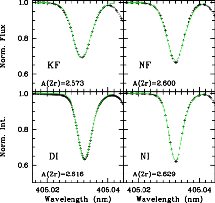
Figure 4: The observed solar disc-integrated (top) and disc-centre (bottom) spectra in the region of the Zr ii line at 405.0 pm (black symbols), superimposed on the best fitting 3D synthetic profile (solid green/grey) obtained with a grid computed with only zirconium.

Figure 5: The observed solar spectrum of Delbouille et al. (1973) for the the Zr ii line at 405.0 pm (dashed black), together with its line bisector (plotted on a ten-times expanded abscissa), superimposed on the 3D synthetic profile (solid black) with its line bisector.

9.3 The Zr ii line at 420.8 nm

This line is strong and sensitive to the adopted damping constants. The red side is more or less clean, while on the blue side there is a weak line, and close by another weak line. The line profile fitting is done with method ’A’, using Zr only, and restricting the fit to the wavelength range $420.891$ …$420.913$ nm in order to avoid the weak blends in the far blue wing of this Zr ii line. The continuum level is fixed in the fitting procedure. The fitting of the disc-integrated line profile in the Kurucz (2005a) spectral atlas is shown in Fig. 6. The abundance derived from line profile fitting and from the EW measured with splot are in very good agreement (within 0.007 dex) for the observed spectra of Delbouille et al. (1973) and Kurucz (2005a). For Neckel & Labs (1984), the abundance from line profile fitting is lower with respect to the abundance derived from the EW measurements by 0.04 dex and and 0.01 dex, for the disc-integrated and disc-centre spectrum, respectively.

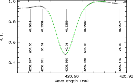
Figure 6: The observed solar disc-integrated spectrum of Kurucz (2005a) (black symbols) in the region of the Zr ii line at 420.8 pm, superimposed on the best fitting profile (solid green/grey) derived from a grid of 3D synthetic spectra computed with only zirconium. The fit corresponds to A(Zr)=2.58.

9.4 The Zr ii line at 425.8 nm

This Zr ii line is on the blue wing of a much stronger Fe ii line that has close by, on the red side, a very strong Fe i line, blended with a weaker Fe ii line (see Fig. 7). We tried different fitting procedures.

First, we fitted the Zr ii line profile with a grid of 3D synthetic profiles computed with only Zr, restricting the fitting to the blue wing of the Zr line. For the disc-centre spectrum of Delbouille et al. (1973) we obtain A(Zr)=$2.65\pm 0.01$. The fit looks quite satisfactory (see Fig. 7), but it is not clear how much the strong lines close by affect the Zr ii line, and hence by how much A(Zr) is overestimated.

Second, we applied method ’B’, taking into account the contribution of the neighbouring iron lines as a linear combination of scaled 3D synthetic profiles, and obtain A(Zr)=$2.61\pm 0.01$.

Finally, we also fitted the complete range with method ’A’, properly taking into account the three iron lines, with A(Zr) and A(Fe) as free fitting parameters. We obtain a Zr abundance of $2.643\pm 0.001$ and $2.627\pm 0.000$ from disc-centre and disc-integrated spectra, respectively. Even though the iron lines are not very well reproduced (see Fig. 8), the Zr ii line is fitted very well and is not affected by the minor deficiencies of the iron lines. The equivalent widths given in Table 3 are derived from the abundances obtained with this fitting method.

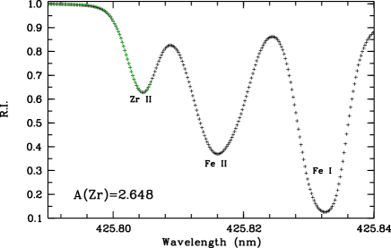
Figure 7: The observed solar disc-centre spectrum of Delbouille et al. (1973) in the region of the Zr ii line at 425.8 pm (black symbols) is superimposed to the 3D best fit (solid green/grey), obtained with a grid of 3D synthetic profiles computed with only Zr.

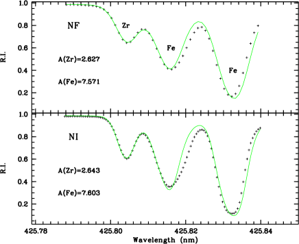
Figure 8: The observed Neckel & Labs (1984) spectrum in the region of the Zr ii line at 425.8 pm (black symbols) is superimposed to the best fitting 3D synthetic spectrum (solid green/grey) obtained with method ’A’. Upper panel: disc-integrated spectrum, lower panel: disc-centre spectrum.

9.5 The Zr ii line at 444.2 nm

This line is surrounded by two stronger features, an iron line on the blue side at 444.2831 nm and a blend of three lines of iron on the red side. Of these three Fe i lines on the red side, the one at 444.3194 nm is much stronger than the other two components.

Clearly, the Zr ii line is affected by the two Fe i features on both sides, and cannot be treated in isolation. Since the two iron features strongly influence the shape of the Zr ii line, the Zr abundance cannot be derived from this line by fitting with a grid of 3D synthetic profiles computed with zirconium only.

The most reliable Zr abundance is obtained from the full fitting, method ’A’: we fitted the observed Fe–Zr–Fe blend with A(Zr) and A(Fe) as free parameters. The Zr abundance derived in this way is $2.673\pm 0.004$ and $2.650\pm 0.005$ for the disc-centre and disc-integrated spectra, respectively (cf. Fig. 9). The equivalent widths given in Table 3 are derived from the abundances of this fitting method.

For completeness, we also derived the Zr abundance with methods ’B’ and ’C’.

For method ’B’, the profiles of the four iron blending features are represented by scaled 3D synthetic Fe line profiles, which are then added to the profile of the Zr ii line in order to obtain an approximate profile of the complete blend (ignoring saturation effects). With this approach, the best fits are obtained with Zr abundances of A(Zr)=$2.67\pm 0.01$ and A(Zr)=$2.64\pm 0.01$ for disc-centre and disc-integrated case, respectively. The fit of the observed disc-integrated spectrum is somewhat better that in the case of the disc-centre observations.

In method ’C’, A(Zr) is found from the equivalent width of the Zr ii line, as obtained from splot with the deblending option. Representing the Fe feature on the red side of the Zr ii line either by a single or by three Voigt profiles turned out to have no influence on the resulting zirconium abundance. We find A(Zr) derived in this way to be very close to the result of method ’B’ in the case of the disc-centre observed spectra. In the disc-integrated case, A(Zr) is about $0.057$ dex smaller than what is obtained with method ’B’.

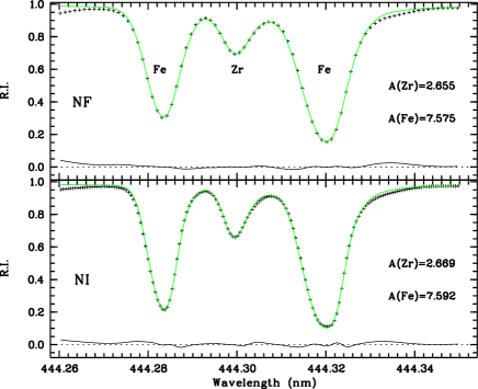
Figure 9: The observed solar disc-centre spectrum of Neckel & Labs (1984) in the region of the Zr ii line at 444.2 pm (black symbols) with the 3D synthetic best-fit-profile obtained with method ’A’ superimposed (solid green/grey). Upper panel: disc-integrated spectrum, lower panel: disc-centre spectrum. The residual is below each plot.

9.6 The Zr ii line at 449.6 nm

This Zr ii line (EW $\approx 3$ pm) is contaminated by a much stronger Cr i line (EW $\approx 9$ pm). Certainly, saturation effects cannot be ignored in this case.

Based on the full 3D line profile fitting of the complete blend using method ’A’, with A(Cr) and A(Zr) as free fitting parameters, we obtain a Zr abundance of A(r)=$2.660\pm 0.003$ for disc-centre (cf. Fig. 11), and A(Zr)=$2.642\pm 0.005$ for integrated disc. These Zr abundances correspond to equivalent widths of 3.11 and 3.41 pm respectively (see Table 3).

The fit resulting from method ’B’, scaling the Cr profile and interpolating in the grid of 3D synthetic Zr profiles to achieve the best agreement between synthetic and observed profile, is shown in Fig. 10 for the disc-centre case. It is of similar quality as the one obtained from the full fitting procedure with method ’A’ (Fig. 11). Method ’B’ gives A(Zr)=$2.63$ and $2.60$ for disc-centre and integrated disc, respectively. As expected, the approximate method ’B’ tends to underestimate the Zr abundance, in this example by $0.027$ and $0.042$ dex for disc-centre and integrated disc, respectively. The average equivalent width we derive with this method for the observed disc-centre and disc-integrated spectra are EW=$3.01$ and $3.25$ pm, respectively, $3.2$ and $4.7$% lower compared to method ’A’.

When we apply method ’C’ using splot with the deblending option, we cannot reproduce the Cr line profile with a single Voigt profile, but we can formally have a good reproduction of the profile with two Voigt profiles, but this option cannot take into account properly the wings of the Cr ii line.

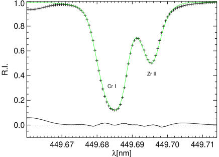
Figure 10: The observed solar disc-centre spectrum of Neckel & Labs (1984) in the region of the Zr ii line at $449.6$ nm (black symbols) with the best fitting 3D synthetic profile obtained from method ’B’ with A(Zr)=2.63 superimposed (solid green/grey). The graph in the lower part shows the synthetic $-$ observed residuals.

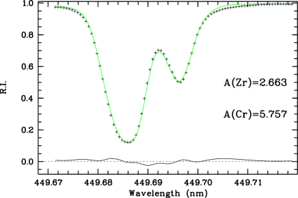
Figure 11: The observed solar disc-centre spectrum of Neckel & Labs (1984) in the region of the Zr ii line at $449.6$ nm (black symbols) with the best fitting 3D synthetic profile obtained from method ’A’ superimposed (solid green/grey). The graph in the lower part shows the synthetic $-$ observed residuals.

9.7 The Zr ii line at 511.2 nm

For this line, the placement of the continuum is difficult, but the uncertainty induces an error in the EW measurement of less than 4% and hence a difference in the Zr abundance of at most 0.02 dex. The line shape suggests that it is blended on both wings, and in fact three weak blend lines are expected according to the Kurucz line list ; two K i lines at 511.2212 and 511.2246 nm, and a Sm ii line at 511.2294 nm. In addition, several weak molecular lines are expected in the range (see Fig. 12).

The average EWs derived with method ’B’ for disc-centre and integrated disc, respectively, are 8.4 and 9.2 pm, corresponding to zirconium abundances of A(Zr)=$2.69$ and $2.67$. When measuring the EW with splot (method ’C’), we find similar results, but the uncertainty in the measurements is larger, giving an indetermination in the abundance determination of about 0.06 dex.

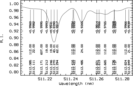
Figure 12: The observed solar disc-centre spectrum of Delbouille et al. (1973) in the region of the Zr ii line at 511.2 nm (black solid) with the identifications of the lines in the range according the line list of Kurucz.

10 Conclusions

We analysed the zirconium abundance in the solar photosphere, investigating a selected sample of lines of both Zr i and Zr ii. The Zr i lines are weak and heavily blended so that only four of them are acceptable for abundance work. However, the present analysis of the zirconium abundance relies primarily on 15 lines of Zr ii that we found suitable for this purpose.

We have applied three different fitting strategies to derive the abundance from Zr lines that are blended by lines of other elements. In the case that all components making up the blend are weak, the different methods give consistent abundances. If, however, stronger lines are involved (for an example see Sect. 9.6), the methods that ignore saturation effects may severely underestimate the Zr abundance by up to $0.05$ dex, even though the result of the fitting may appear pleasing to the eye, and the reduced $\chi^{2}$ may be close to one.

We find a good agreement between A(Zr) derived from the Zr i and the Zr ii lines, but, due to the scarcity of Zr i lines, we consider this result as fortuitous. The abundance from disc-centre spectra is systematically higher than the one from disc-integrated observations. A similar result is also found for other heavy elements like Fe, Th, Hf, both with 3D and 1D model atmospheres. This may indicate a problem with the thermal structure of the models, rather than a physical abundance gradient in the solar atmosphere. Further investigations are necessary to find an explanation for this small discrepancy.

Our recommended solar zirconium abundance is based on the 3D result for 15 Zr ii lines, and is A(Zr)$=2.62\pm 0.06$, where the uncertainty is the line-to-line scatter of the selected sample of Zr ii lines. This value is at the upper end of the solar zirconium abundances found in the literature. Still, within the mutual error bars, this result is in good agreement with the meteoritic zirconium abundance of A(Zr)=$2.57\pm 0.04$ (Lodders et al. 2009).