Improved linear programming decoding of LDPC codes and bounds on the minimum and fractional distance

Abstract

We examine LDPC codes decoded using linear programming (LP). Four contributions to the LP framework are presented. First, a new method of tightening the LP relaxation, and thus improving the LP decoder, is proposed. Second, we present an algorithm which calculates a lower bound on the minimum distance of a specific code. This algorithm exhibits complexity which scales quadratically with the block length. Third, we propose a method to obtain a tight lower bound on the fractional distance, also with quadratic complexity, and thus less than previously-existing methods. Finally, we show how the fundamental LP polytope for generalized LDPC codes and nonbinary LDPC codes can be obtained.

This research was supported by the Israel Science Foundation, grant no. 772/09.

I Introduction

Within the field of error-correcting codes, the method of linear programming (LP) decoding of linear codes has attracted considerable attention in recent years. Over the past several years, this method has stirred a substantial amount of research. One reason for this is that the LP decoder has the ML certificate property [1], i.e., that if the LP decoder succeeds in producing an integral solution vector, then it produces the ML solution. Another attractive property of the LP decoder is that one may improve the performance in various ways. These include using generic techniques to tighten the LP relaxations [1], using integer programming or mixed integer linear programming [1], [2], adding constraints to the Tanner graph [3] and guessing facets of the polytope [4].

However, LP decoding is disadvantaged as compared to iterative decoding algorithms such as belief propagation or min-sum decoding because the decoding complexity can be much larger. In general the LP decoder entails a polynomial, non-linear complexity. Several authors have proposed algorithms for low-complexity LP decoding, e.g. [5], [6], [7]. Vontobel and Koetter [5] have proposed an iterative, Gauss-Seidel-type algorithm for approximate LP decoding. In [8] the approach of [5] was studied under a newly-proposed scheduling scheme. This study showed that the performance of the LP decoder can be approached with linear computational complexity. It was also shown that the iterative LP decoder can correct a fixed fraction of errors with linear computational complexity. These results were also extended to generalized LDPC (GLDPC) codes.

In this paper, we present the following main results. First, we show that merging check nodes in the graph can tighten the relaxation and improve the LP decoder. Second, we demonstrate how the linear-complexity LP decoder from [8] can be used to obtain a lower bound on the minimum distance of a specific code, which is also an upper bound on the fractional distance of the code, with complexity $O(N^{2})$, where $N$ is the block length. This lower bound on the minimum distance can be improved by using the check node merging technique. Third, we propose an algorithm which calculates a tight lower bound on the fractional distance with complexity $O(N^{2})$. We note that Feldman $et\,\,al.\,\,$[1] were the first to propose an algorithm which calculates the exact fractional distance; their algorithm entails a complexity which is polynomial but not quadratic in the block length. This is also true for the fractional distance calculation in [7], even though it has reduced complexity as compared to [1]. Our approach has lower complexity as compared to these techniques. Finally, we show how the fundamental polytope of two important classes of codes, namely GLDPC and nonbinary codes, can be obtained. This is accomplished by using the double description method [9, 10]. In addition to these results, we show how the linear-complexity LP decoder can be calculated efficiently for GLDPC codes.

This paper is organized as follows. In section II the linear-complexity LP decoder [8] is reviewed. Section III shows how to perform some computations relating to the linear-complexity LP decoder in an efficient manner. Section IV describes how improved LP decoding can be achieved by merging check nodes. In Section V we propose an algorithm which yields a lower bound on the minimum distance which is also an upper bound on the fractional distance of specific LDPC codes. In Section VI, an algorithm which produces a tight lower bound on the fractional distance is presented. We show how to obtain the fundamental polytope of GLDPC and nonbinary codes in Section VII. Section VIII provides some numerical results, and the paper is concluded in Section IX.

II Approximate Iterative Linear programming decoding of GLDPC codes

Consider a discrete binary-input memoryless channel (DMC) described by the probability transition function $Q(y\>|\>c)$ where $c$ is the transmitted code-bit and $y$ is the channel output. Also consider a GLDPC code ${\mathcal{C}}$ represented by a Tanner graph with $N$ variable nodes and $M$ linear constraint nodes, where each constraint node represents a small local constituent code, thus generalizing single parity checks (SPCs) in plain LDPC codes. The code ${\mathcal{C}}$ is used to transmit information over the given DMC. Following the notation in [1], let ${\mathcal{I}}$ and ${\cal J}$ be the sets of variable and constraint nodes, respectively, such that $|{\mathcal{I}}|=N$ and $|{\cal J}|=M$. The variable node $i\in{\mathcal{I}}$ is connected to the set ${\mathcal{N}}_{i}$ of constraint node neighbors. The constraint node $j\in{\cal J}$ is connected to the set ${\mathcal{N}}_{j}$ of constraint node neighbors. Further denote by ${\bf c}_{j}$ the vector

$${\bf c}_{j}\>{\stackrel{{\scriptstyle\scriptscriptstyle\Delta}}{{=}}}\>\{c_{i}\}_{i\in{\mathcal{N}}_{j}}\>.$$ (1)

Given some $j\in{\cal J}$, denote by ${\mathcal{C}}_{j}$ the constituent binary linear code corresponding to the constraint node $j\in{\cal J}$ (thus for plain LDPC codes, ${\mathcal{C}}_{j}$ is a simple parity-check code). Let ${\bf 0}_{j}$ denote the all-zero local codeword on constraint node $j$, and let ${\bf 0}$ denote the all-zero codeword in ${\mathcal{C}}$. A valid codeword ${\bf c}\in{\mathcal{C}}$ satisfies ${\bf c}_{j}\in{\mathcal{C}}_{j}$, $\forall j\in{\cal J}$.

We assume, without loss of generality, that there are no parallel edges in the Tanner graph, since otherwise we can modify the structure of the code to satisfy this constraint.

The LP decoder is given by [1],

$${\hat{\bf c}}\>{\stackrel{{\scriptstyle\scriptscriptstyle\Delta}}{{=}}}\>\mathop{\rm argmin}_{{\bf c},\mbox{\boldmath$\omega$}}{\rm P}({\bf c})$$ (2)

where the vector $\omega$ is defined by

$$\mbox{\boldmath$\omega$}\>{\stackrel{{\scriptstyle\scriptscriptstyle\Delta}}{{=}}}\>\{w_{j,{\bf{g}}}\}_{j\in{\cal J},\>{\bf{g}}\in{\mathcal{C}}_{j}}$$

and where

$${\rm P}({\bf c})\>{\stackrel{{\scriptstyle\scriptscriptstyle\Delta}}{{=}}}\>\sum_{i\in{\mathcal{I}}}c_{i}\gamma_{i}$$ (3)

subject to

$$w_{j,{\bf{g}}}\geq 0\qquad\forall j\in{\cal J}\>,\>{\bf{g}}\in{\mathcal{C}}_{j}$$ (4)

$$\sum_{{\bf{g}}\in{\mathcal{C}}_{j}}w_{j,{\bf{g}}}=1\qquad\forall j\in{\cal J}$$ (5)

$$c_{i}=\sum_{{\bf{g}}\in{\mathcal{C}}_{j}\>,\>g_{i}=1}w_{j,{\bf{g}}}\qquad\forall j\in{\cal J}\>,\>i\in{\mathcal{N}}_{j}$$ (6)

and where

$$\gamma_{i}\>{\stackrel{{\scriptstyle\scriptscriptstyle\Delta}}{{=}}}\>\log\frac{Q(y_{i}\>|\>0)}{Q(y_{i}\>|\>1)}$$

where all logarithms henceforth are to the base $e$. We assume that there are no perfect measurements from the channel, i.e.

$$-\infty<\gamma_{i}<\infty\qquad\forall i\in{\mathcal{I}}\>.$$ (7)

Note that if we transmit over the binary erasure channel (BEC) then this assumption does not hold. However, we can re-normalize the $\gamma_{i}$’s by replacing $\gamma_{i}=\infty$ with $\gamma_{i}=1$ and $\gamma_{i}=-\infty$ with $\gamma_{i}=-1$. After this re-normalization the assumption (7) holds, and we can then apply the decoding algorithm.

We term the minimization problem (2)-(6), Problem-P. We also define

$$\mbox{\boldmath$\omega$}_{j}\>{\stackrel{{\scriptstyle\scriptscriptstyle\Delta}}{{=}}}\>\{w_{j,{\bf{g}}}\}_{{\bf{g}}\in{\mathcal{C}}_{j}}$$

The polytope ${\cal Q}_{j}({\mathcal{C}})$ is defined as follows [1]: ${\bf c}\in{\cal Q}_{j}({\mathcal{C}})$ (sometimes we will use the notation ${\bf c}_{j}\in{\cal Q}_{j}({\mathcal{C}})$, the meaning will be clear from the context) if and only if there exists a vector $\mbox{\boldmath$\omega$}_{j}$ such that (4)-(6) hold for this value of $j$. For plain LDPC codes it was shown that ${\bf c}\in{\cal Q}_{j}({\mathcal{C}})$ if and only if

$$\begin{array}[]{l l}0\leq c_{i}\leq 1&\forall i\in{\mathcal{N}}_{j}\\ \sum_{i\in{\mathcal{N}}_{j}\setminus S}c_{i}+\sum_{i\in S}\left(1-c_{i}\right)\geq 1&\forall S\subseteq{\mathcal{N}}_{j}\>,|S|\>{\rm odd}\end{array}$$ (8)

We further denote by ${\cal Q}({\mathcal{C}})\>{\stackrel{{\scriptstyle\scriptscriptstyle\Delta}}{{=}}}\>\bigcap_{j\in{\cal J}}{\cal Q}_{j}({\mathcal{C}})$ the relaxed [1] or fundamental polytope. Thus ${\bf c}$ is feasible in (4)-(6) if and only if ${\bf c}\in{\cal Q}({\mathcal{C}})$. We thus have, in addition to (2), the relation

$$\hat{\bf c}=\mathop{\rm argmin}_{{\bf c}\in{\cal Q}({\mathcal{C}})}{\rm P}({\bf c})$$ (9)

An important observation is that the LP decoder has the ML certificate [1] in the sense that if the solution of Problem-P is integer (in fact an integer $\omega$ implies that ${\bf c}$ is also integer by (6)) then it is the ML decision.

Now consider the following problem, which we term Problem-D. The variables in this problem are

$${\bf u}=\{u_{i,j}\}_{i\in{\mathcal{I}},j\in{\mathcal{N}}_{i}}$$

and the problem is defined by

$$\max_{{\bf u}}{\rm D}({\bf u})\quad{\rm where}\quad{\rm D}({\bf u})\>{\stackrel{{\scriptstyle\scriptscriptstyle\Delta}}{{=}}}\>\sum_{j\in{\cal J}}\min_{{\bf{g}}\in{\mathcal{C}}_{j}}\left\{\sum_{i\in{\mathcal{N}}_{j}}u_{i,j}g_{i}\right\}$$ (10)

subject to

$$\sum_{j\in{\mathcal{N}}_{i}}u_{i,j}=\gamma_{i}\qquad\forall i\in{\mathcal{I}}\>.$$ (11)

Lemma 1

Problem-P and Problem-D are Lagrange dual problems. The minimum of Problem-P is equal to the maximum of Problem-D.

The lemma is proven in [8].

Vontobel and Koetter [5] have proposed an algorithm which yields an approximated solution to Problem-D. They suggested to consider the following “soft” version of Problem-D, termed Problem-DS:

$$\max_{{\bf u}}{\rm DS}({\bf u})$$

where

$${\rm DS}({\bf u})\>{\stackrel{{\scriptstyle\scriptscriptstyle\Delta}}{{=}}}\>-\frac{1}{K}\sum_{j\in{\cal J}}\log\sum_{{\bf{g}}\in{\mathcal{C}}_{j}}e^{-K\sum_{i\in{\mathcal{N}}_{j}}u_{i,j}g_{i}}$$ (12)

subject to (11). Note that the objective function in (12) is obtained from (10) by approximating the $\min()$ function using a log-sum-exp function with a parameter $K>0$. This approximation can become arbitrarily accurate by increasing $K$. Also note that ${\rm DS}({\bf u})$ is concave since the log-sum-exp function is convex. In what follows, we give a brief overview of the linear-complexity iterative LP decoder. The reader is referred to [8] for additional details.

Let $\tilde{\Psi}^{j}$ denote the $(|{\mathcal{N}}_{j}|+1)\times|{\mathcal{C}}_{j}|$ matrix

$$\tilde{\Psi}^{j}\>{\stackrel{{\scriptstyle\scriptscriptstyle\Delta}}{{=}}}\>\left(\begin{array}[]{c}{\bf 1}_{|{\mathcal{C}}_{j}|}\\ \Psi^{j}\end{array}\right)$$ (13)

where ${\bf 1}_{|{\mathcal{C}}_{j}|}$ is a row vector of $|{\mathcal{C}}_{j}|$ ones and the columns of $\Psi^{j}$ are all the codewords of ${\mathcal{C}}_{j}$.

Note that the equation set

$$\left(\begin{array}[]{c}1\\ {\bf c}_{j}\end{array}\right)=\tilde{\Psi}^{j}\mbox{\boldmath$\omega$}_{j}$$

expresses the constraints (5)-(6). We define

$$\Xi^{j}\>{\stackrel{{\scriptstyle\scriptscriptstyle\Delta}}{{=}}}\>\left(\tilde{\Psi}^{j}\right)^{T}\left(\tilde{\Psi}^{j}\left(\tilde{\Psi}^{j}\right)^{T}\right)^{-1}$$

where $A^{T}$ is the transpose of matrix $A$, and

$$\eta\>{\stackrel{{\scriptstyle\scriptscriptstyle\Delta}}{{=}}}\>\max_{j}\left\{|{\mathcal{C}}_{j}||{\mathcal{N}}_{j}|\max_{l,i}|\Xi^{j}_{l,i}|\right\}$$

where $\Xi^{j}_{l,i}$ is the $(l,i)$ element of $\Xi^{j}$.

Now let $\epsilon>0$ be a constant such that $\epsilon\leq 1/\eta$. We define

$$\tilde{\lambda}_{i}\>{\stackrel{{\scriptstyle\scriptscriptstyle\Delta}}{{=}}}\>\lambda_{i}(1-\eta\epsilon)+\frac{\eta}{2}\epsilon\qquad\forall i\in{\mathcal{I}}$$ (14)

and

$$\tilde{\mbox{\boldmath$\lambda$}}\>{\stackrel{{\scriptstyle\scriptscriptstyle\Delta}}{{=}}}\>\{\tilde{\lambda}_{i}\}_{i\in{\mathcal{I}}}\>.$$

We will also define the quantities

$$A_{k,j} \>{\stackrel{{\scriptstyle\scriptscriptstyle\Delta}}{{=}}}\> \sum_{{\bf{g}}\in{\mathcal{C}}_{j},\>g_{k}=1}e^{-K\sum_{i\in{\mathcal{N}}_{j}\setminus k}u_{i,j}g_{i}}$$

$$B_{k,j} \>{\stackrel{{\scriptstyle\scriptscriptstyle\Delta}}{{=}}}\> \sum_{{\bf{g}}\in{\mathcal{C}}_{j},\>g_{k}=0}e^{-K\sum_{i\in{\mathcal{N}}_{j}\setminus k}u_{i,j}g_{i}}$$ (15)

The following iterative algorithm was proposed in [8] to find an approximate solution to Problem-P in linear time complexity.

Algorithm 1

Given a GLDPC code, channel observations and some fixed parameters $\epsilon_{0}\in(0,1/\eta)$ and $K>0$ do:

1. Initialization:

   $$\forall i\in{\mathcal{I}},j\in{\mathcal{N}}_{i}\>:\>\> u_{i,j}=\gamma_{i}/|{\mathcal{N}}_{i}|$$

   $$\forall i\in{\mathcal{I}},j\in{\mathcal{N}}_{i}\>:\>\> v_{i,j}=-\frac{1}{K}\log\frac{B_{i,j}}{A_{i,j}}$$

   $$\forall i\in{\mathcal{I}},j\in{\mathcal{N}}_{i}\>:\>\> \lambda_{i,j}=\frac{1}{1+e^{K(u_{i,j}-v_{i,j})}}$$

   $$\forall i\in{\mathcal{I}}\>:\>\> \lambda_{i}=\frac{1}{|{\mathcal{N}}_{i}|}\sum_{j\in{\mathcal{N}}_{i}}\lambda_{i,j}$$

   $$\forall i\in{\mathcal{I}}\>:\>\> \epsilon_{i}=\max_{j\in{\mathcal{N}}_{i}}|\lambda_{i,j}-\lambda_{i}|$$

   $${\cal A}=\{i\in{\mathcal{I}}\>:\>\epsilon_{i}\geq\epsilon_{0}\}$$

2. Iteration: Pick an arbitrary element $k\in{\cal A}$ and make the following updates:

   $$\forall j\in{\mathcal{N}}_{k}:\>u_{k,j}=v_{k,j}+\frac{\gamma_{k}}{|{\mathcal{N}}_{k}|}-\frac{1}{|{\mathcal{N}}_{k}|}\sum_{l\in{\mathcal{N}}_{k}}v_{k,l}$$

   $$\forall i\in{\mathcal{N}}_{j}\setminus k,j\in{\mathcal{N}}_{k}:\>v_{i,j}=-\frac{1}{K}\log\frac{B_{i,j}}{A_{i,j}}$$

   $$\forall i\in{\mathcal{N}}_{j},j\in{\mathcal{N}}_{k}:\>\lambda_{i,j}=\frac{1}{1+e^{K(u_{i,j}-v_{i,j})}}$$

   $$\forall i\in{\mathcal{N}}_{j},j\in{\mathcal{N}}_{k}:\>\lambda_{i}=\frac{1}{|{\mathcal{N}}_{i}|}\sum_{j^{\prime}\in{\mathcal{N}}_{i}}\lambda_{i,j^{\prime}}$$

   $$\forall i\in{\mathcal{N}}_{j},j\in{\mathcal{N}}_{k}:\>\epsilon_{i}=\max_{j^{\prime}\in{\mathcal{N}}_{i}}|\lambda_{i,j^{\prime}}-\lambda_{i}|$$

   $$\forall i\in{\mathcal{N}}_{j},j\in{\mathcal{N}}_{k}:\>\mbox{If }i\in{\cal A}\mbox{ and }\epsilon_{i}<\epsilon_{0}\mbox{ then }{\cal A}={\cal A}\setminus i$$

   $$\forall i\in{\mathcal{N}}_{j},j\in{\mathcal{N}}_{k}:\>\mbox{If }i\not\in{\cal A}\mbox{ and }\epsilon_{i}\geq\epsilon_{0}\mbox{ then }{\cal A}={\cal A}\cup i$$

3. Loop Control: If ${\cal A}\neq\emptyset$ then repeat step 2. Otherwise proceed to step 4.

4. Produce the final solution and Exit: $\forall i\in{\mathcal{I}}$ : Compute $\tilde{\lambda}_{i}$ using (14), and $\hat{c}_{i}$ using

   $$\hat{c}_{i}=\left\{\begin{array}[]{ll}1&\hbox{if $\tilde{\lambda}_{i}>0.5$}\\ 0&\hbox{if $\tilde{\lambda}_{i}<0.5$}\end{array}\right.$$

   Output the primal vector $\tilde{\mbox{\boldmath$\lambda$}}$, the dual vector ${\bf u}$ and the bitwise-estimated integral vector $\{\hat{c}_{i}\}_{i\in{\mathcal{I}}}$

Note that each edge in the graph connecting the variable node $i$ and the constraint node $j$ is associated with the variables $u_{i,j}$, $v_{i,j}$ and $\lambda_{i,j}$. Each variable node $i\in{\mathcal{I}}$ is associated with the variables $\lambda_{i}$, $\tilde{\lambda}_{i}$, $\hat{c}_{i}$ and $\epsilon_{i}$. In [8] the following assumptions were made.

1. $$|\gamma_{i}|\leq\gamma_{\max}\qquad\forall i\in{\mathcal{I}}$$ (16)

   for some positive constant $\gamma_{\max}$. Note that practical channels with non-perfect measurements, that satisfy (7), also satisfy (16), since their output is quantized to some finite set.

2. As was indicated earlier, we can assume without loss of generality that there are no parallel edges in the Tanner graph.

3. We assume that $d^{\prime}_{j}\geq 3$ $\forall j\in{\cal J}$. where $d^{\prime}_{j}$ is the dual distance of the constituent code corresponding to the constraint node $j$. For plain LDPC codes this assumption degenerates to $|{\mathcal{N}}_{j}|\geq 3$ $\forall j\in{\cal J}$ (this simpler version appears also in [5]).

4. We assume that all node degrees are bounded by some constant (independent of $N$).

Under these assumptions it was shown in [8], for any fixed $\epsilon_{0}\in(0,1/\eta)$ and $K>0$, that Algorithm 1 exits after $O(N)$ iterations, and that the vector $\tilde{\mbox{\boldmath$\lambda$}}$ is feasible in Problem-P. Furthermore, by setting $K$ sufficiently large and $\epsilon_{0}$ sufficiently small, we can make $(P(\tilde{\mbox{\boldmath$\lambda$}})-P^{\ast})/N$, where ${\rm P}^{\ast}$ is the minimum value of Problem-P, arbitrarily small. More precisely,

[8, Theorem 1]: Consider Algorithm 1 under the four assumptions above. For any given $\delta$, after $O(N)$ iterations, each with a constant number of operations, the algorithm yields a vector, $\tilde{\mbox{\boldmath$\lambda$}}$, which is feasible in Problem-P and satisfies

$$0\leq{\rm P}(\tilde{\mbox{\boldmath$\lambda$}})-{\rm P}^{\ast}\leq\delta N$$ (17)

By weak duality and by the primal feasibility of $\tilde{\mbox{\boldmath$\lambda$}}$, we have

$${\rm D}({\bf u})\leq{\rm P}^{\ast}\leq{\rm P}(\tilde{\mbox{\boldmath$\lambda$}})$$ (18)

We will make use of the fact that ${\rm P}^{\ast}$ is sandwiched between the lower bound ${\rm D}({\bf u})$ and the upper bound ${\rm P}(\tilde{\mbox{\boldmath$\lambda$}})$. In fact, in the proof of [8, Theorem 1], it was shown that

$${\rm P}(\tilde{\mbox{\boldmath$\lambda$}})-{\rm D}({\bf u})\leq\delta N$$ (19)

and thus follows the result of the theorem.

III Efficient computations related to the iterative approximate LP decoder

In this section, we demonstrate how the computation of $A_{k,j}$ and $B_{k,j}$, defined in (II) can be efficiently implemented for GLDPC codes. For LDPC codes an efficient computation scheme was presented in [8]. We also show how to efficiently implement the calculation of ${\rm D}({\bf u})$.

We follow the approach proposed in [11] that uses a trellis representation of the code. To simplify the notation we assume that ${\mathcal{N}}_{j}=\{0,1,\ldots,n-1\}$, and we fix $j$ and omit it from $A_{k,j}$, $B_{k,j}$, ${\mathcal{C}}_{j}$ and $u_{i,j}$. In addition we assume that the code ${\mathcal{C}}_{j}$ is represented by the parity check matrix

$$H=\left[{\bf h}_{0}\>{\bf h}_{1}\>\ldots\>{\bf h}_{n-1}\right]$$

with columns ${\bf h}_{0},{\bf h}_{1},\ldots,{\bf h}_{n-1}$, such that the vectors ${\bf h}_{i}$ are $m$-dimensional binary vectors representing elements of the field ${\rm GF}(2^{m})$.

III-A Efficient Computation of $A_{k,j}$ and $B_{k,j}$

We need to compute $A_{k}$ and $B_{k}$, $k=0,1,\ldots,n-1$, defined by

$$A_{k} \>{\stackrel{{\scriptstyle\scriptscriptstyle\Delta}}{{=}}}\> \sum_{{\bf{g}}\>:\>H{\bf{g}}=0,\>g_{k}=1}e^{-K\left(\sum_{i=0}^{n-1}u_{i}g_{i}-u_{k}\right)}$$

$$B_{k} \>{\stackrel{{\scriptstyle\scriptscriptstyle\Delta}}{{=}}}\> \sum_{{\bf{g}}\>:\>H{\bf{g}}=0,\>g_{k}=0}e^{-K\sum_{i=0}^{n-1}u_{i}g_{i}}\>.$$ (20)

where ${\bf{g}}\>{\stackrel{{\scriptstyle\scriptscriptstyle\Delta}}{{=}}}\>\left[g_{0},g_{1},\ldots,g_{n-1}\right]^{T}$

Let $H_{k}$, ${\bf{g}}_{k}$, $E(k,{\bf s})$ and $E(k,{\bf s},b)$ be defined by

$$H_{k}\>{\stackrel{{\scriptstyle\scriptscriptstyle\Delta}}{{=}}}\>\left[{\bf h}_{0}\>{\bf h}_{1}\>\ldots\>{\bf h}_{k}\right]\quad,\quad{\bf{g}}_{k}\>{\stackrel{{\scriptstyle\scriptscriptstyle\Delta}}{{=}}}\>\left[g_{0},g_{1},\ldots,g_{k}\right]^{T}$$ (21)

$$E(k,{\bf s})=\sum_{{\bf{g}}_{k}\>:\>H_{k}{\bf{g}}_{k}={\bf s}}e^{-K\sum_{i=0}^{k}u_{i}g_{i}}$$

and

$$E(k,{\bf s},b) = \sum_{{\bf{g}}_{k}\>:\>H_{k}{\bf{g}}_{k}={\bf s},g_{k}=b}e^{-K\sum_{i=0}^{k}u_{i}g_{i}}$$ (22)

$$= E(k-1,{\bf s}\oplus b\cdot{\bf h}_{k})e^{-Ku_{k}\cdot b}$$

In these definitions ${\bf s}$ is an $m$ dimensional binary vector, representing an element in ${\rm GF}(2^{m})$, $b\in\{0,1\}$, $g_{i}\in\{0,1\}$, and $\oplus$ is the bitwise exclusive or operator (addition in ${\rm GF}(2^{m})$).

Similarly we define

$$\tilde{H}_{k} \>{\stackrel{{\scriptstyle\scriptscriptstyle\Delta}}{{=}}}\> \left[{\bf h}_{k+1}\>{\bf h}_{k+2}\>\ldots\>{\bf h}_{n-1}\right]$$

$$\tilde{{\bf{g}}}_{k} \>{\stackrel{{\scriptstyle\scriptscriptstyle\Delta}}{{=}}}\> \left[g_{k+1},g_{k+2},\ldots,g_{n-1}\right]^{T}$$ (23)

$$\tilde{E}(k,{\bf s})=\sum_{\tilde{{\bf{g}}}_{k}\>:\>\tilde{H}_{k}\tilde{{\bf{g}}}_{k}={\bf s}}e^{-K\sum_{i=k+1}^{n-1}u_{i}g_{i}}$$

$E(k,{\bf s})$ and $\tilde{E}(k,{\bf s})$ can be computed recursively using the forward recursion for $k=0,1,\ldots,n-1$

$$E(k,{\bf s})=E(k-1,{\bf s})+E(k-1,{\bf s}\oplus{\bf h}_{k})\cdot e^{-Ku_{k}}$$ (24)

(for a given value of $k$ we use this recursion to compute $E(k,{\bf s})$ for all possible states ${\bf s}$) and the backward recursion for $k=n-2,\ldots,1,0$

$$\tilde{E}(k,{\bf s})=\tilde{E}(k+1,{\bf s})+\tilde{E}(k+1,{\bf s}\oplus{\bf h}_{k+1})\cdot e^{-Ku_{k+1}}$$ (25)

and the initial conditions

$$E(-1,{\bf s})=\left\{\begin{array}[]{ll}1,&\hbox{{\bf s}=0}\\ 0,&\hbox{otherwise}\end{array}\right.$$ (26)

and

$$\tilde{E}(n-1,{\bf s})=\left\{\begin{array}[]{ll}1,&\hbox{{\bf s}=0}\\ 0,&\hbox{otherwise}\end{array}\right.$$ (27)

Finally, $A_{k}$ and $B_{k}$ are computed using

$$A_{k}=e^{Ku_{k}}\sum_{{\bf s}}E(k,{\bf s},1)\tilde{E}(k,{\bf s})$$ (28)

and

$$B_{k}=\sum_{{\bf s}}E(k,{\bf s},0)\tilde{E}(k,{\bf s})$$ (29)

for $k=0,\ldots,n-1$.

In practice, in order to avoid numerical problems, the forward recursion (24) and the backward recursion (25) are computed using logarithmic computation.

Another possibility is to use the method proposed by Hartmann and Rudolph [12]. However, in this case one faces a numerical problem since the method involves subtractions, and not only summations.

III-B Efficient calculation of ${\rm D}({\bf u})$

To calculate ${\rm D}({\bf u})$ for GLDPC codes, we use the same methodology as in the calculation of $A_{k,j}$ and $B_{k,j}$, and we use the definitions of $H_{k}$ and ${\bf{g}}_{k}$ in (21). The difference is that here we only need a forward recursion for the calculation.

By defining

$$A(k,{\bf s})\>{\stackrel{{\scriptstyle\scriptscriptstyle\Delta}}{{=}}}\>\min_{{\bf{g}}_{k}:\;H_{k}{\bf{g}}_{k}={\bf s}}\sum_{i=0}^{n-1}u_{i}g_{i}$$

it is easily seen that our objective (the minimization in (10)) is equal to

$$A(n-1,0)$$ (30)

Now, $A(k,{\bf s})$ can be calculated recursively for $k=0,1,\dots,n-1$ as

$$A(k,{\bf s})=\min(A(k-1,{\bf s}),A(k-1,{\bf s}\oplus{\bf h}_{k})+u_{k})$$

with the initial conditions

$$A(-1,{\bf s})=\left\{\begin{array}[]{ll}0,&\hbox{{\bf s}=0}\\ \infty,&\hbox{otherwise}\end{array}\right.$$ (31)

IV A new method for improved LP decoding

Consider some GLDPC code ${\mathcal{C}}$ with an underlying Tanner graph $\mathcal{G}$. Let $\hat{\bf c}$ be the LP decoded word considered in Section II, i.e.

$$\hat{\bf c}=\mathop{\rm argmin}_{{\bf c}\in{\cal Q}({\mathcal{C}})}{\rm P}({\bf c})$$

where

$${\cal Q}({\mathcal{C}})=\\ \left\{{\bf c}\>:\>\exists\mbox{\boldmath$\omega$}=\left\{w_{j,S}\right\}_{j\in{\cal J},\>S\in{\cal E}_{j}}\mbox{ s.t. \eqref{eq:positive_w}, \eqref{eq:w_sum_1} and \eqref{eq:ci} hold}\right\}$$

Now suppose that we merge some of the constraint nodes together to form an alternative representation of the given code, with underlying graph $\mathcal{G}^{\prime}$. This is illustrated in Figure 1, where we merge the constraint nodes $j_{1}$ and $j_{2}$ into $j^{\prime}_{1}$ (i.e. the constituent code associated with $j^{\prime}_{1}$ satisfies both the constraints implied by $j_{1}$ and those implied by $j_{2}$), and the constraint nodes $j_{3}$ and $j_{4}$ into $j^{\prime}_{2}$. In this example the constraint node $j_{5}$ is left unchanged ($j^{\prime}_{3}$ in $\mathcal{G}^{\prime}$).

Figure 1: Starting from the graph $\mathcal{G}$ on the left part of the figure that represents the code ${\mathcal{C}}$, we merge constraint nodes, thus creating a new representation of ${\mathcal{C}}$ with an underlying graph $\mathcal{G}^{\prime}$ shown on the right.

Denote by ${\cal J}^{\prime}$ the new set of constraint nodes corresponding to $\mathcal{G}^{\prime}$. Now, we can apply the LP relaxation to the new representation and calculate $\hat{\bf c}^{\prime}$ defined by,

$$\hat{\bf c}^{\prime}=\mathop{\rm argmin}_{{\bf c}\in{\cal Q}^{\prime}({\mathcal{C}})}{\rm P}({\bf c})$$

where

$${\cal Q}^{\prime}({\mathcal{C}})=\left\{{\bf c}\>:\>\exists\mbox{\boldmath$\omega$}=\left\{w^{\prime}_{j,{\bf{g}}}\right\}_{j\in{\cal J}^{\prime},\>{\bf{g}}\in{\mathcal{C}}_{j}^{\prime}}\mbox{ s.t. \eqref{eq:positive_w}, \eqref{eq:w_sum_1} }\right.\\ \left.\mbox{ and \eqref{eq:ci} (with ${\cal J}^{\prime},{\mathcal{C}}_{j}^{\prime}$ instead of ${\cal J},{\mathcal{C}}_{j}$) hold}\right\}$$

Proposition 1

${\cal Q}^{\prime}({\mathcal{C}})\subseteq{\cal Q}({\mathcal{C}})$.

Proof: Suppose that ${\bf c}\in{\cal Q}^{\prime}({\mathcal{C}})$. We need to show that ${\bf c}\in{\cal Q}({\mathcal{C}})$. First suppose that the only difference between $\mathcal{G}$ and $\mathcal{G}^{\prime}$ is that the constraint nodes $j_{1},j_{2},\ldots,j_{r}\in{\cal J}$ in $\mathcal{G}$ are merged to form the constraint node $j^{\prime}\in{\cal J}^{\prime}$ in $\mathcal{G}^{\prime}$. All the other constraint nodes in $\mathcal{G}$ and $\mathcal{G}^{\prime}$ are identical (i.e. they are associated with the same constituent codes and are connected to the same variable nodes). Now, there exists $\left\{w^{\prime}_{j,{\bf{g}}}\right\}_{j\in{\cal J}^{\prime},\>{\bf{g}}\in{\mathcal{C}}_{j}^{\prime}}$ such that (4), (5) and (6) (with ${\cal J}^{\prime},{\mathcal{C}}_{j}^{\prime}$ instead of ${\cal J},{\mathcal{C}}_{j}$) hold. For $j=j_{1},j_{2},\ldots,j_{r}$, define $w_{j,{\bf{g}}}$ by,

$$w_{j,{\bf{g}}}\>{\stackrel{{\scriptstyle\scriptscriptstyle\Delta}}{{=}}}\>\sum_{{\bf{g}}^{\prime}\in{\mathcal{C}}_{j}^{\prime},\>{\bf{g}}^{\prime}_{{\mathcal{N}}_{j}}={\bf{g}}}w^{\prime}_{j^{\prime},{\bf{g}}^{\prime}}$$

where ${\bf{g}}^{\prime}_{{\mathcal{N}}_{j}}$ is the sub-codeword ${\bf{g}}^{\prime}$ restricted to indices $i\in{\mathcal{N}}_{j}$. For all other values of $j\in{\cal J}$ we define $w_{j,{\bf{g}}}=w^{\prime}_{j^{\prime}(j),{\bf{g}}}$ where $j^{\prime}(j)\in{\cal J}^{\prime}$ is the constraint node in $\mathcal{G}^{\prime}$ that corresponds to the constraint node $j\in{\cal J}$ in $\mathcal{G}$.

Note that ${\bf{g}}^{\prime}\in{\mathcal{C}}_{j}^{\prime}$ only if ${\bf{g}}^{\prime}_{{\mathcal{N}}_{j}}\in{\mathcal{C}}_{j}$ (since any codeword associated with the merged node $j^{\prime}$ is a codeword of ${\mathcal{C}}_{j}$ for all $j=j_{1},\ldots,j_{r}$). It follows that for all $j=j_{1},\ldots,j_{r}$,

$$w_{j,{\bf{g}}}\geq 0$$

$$\sum_{{\bf{g}}\in{\mathcal{C}}_{j}}w_{j,{\bf{g}}}=\sum_{{\bf{g}}^{\prime}\in{\mathcal{C}}_{j}^{\prime}}w^{\prime}_{j^{\prime},{\bf{g}}^{\prime}}=1$$

$$\sum_{{\bf{g}}\in{\mathcal{C}}_{j}\>,\>g_{i}=1}w_{j,{\bf{g}}}=\sum_{{\bf{g}}^{\prime}\in{\mathcal{C}}_{j}^{\prime}\>,\>g^{\prime}_{i}=1}w^{\prime}_{j^{\prime},{\bf{g}}^{\prime}}=c_{i}\qquad\forall i\in{\mathcal{N}}_{j}$$

Hence we conclude that ${\bf c}\in{\cal Q}({\mathcal{C}})$. We have therefore shown that in this case ${\cal Q}^{\prime}({\mathcal{C}})\subseteq{\cal Q}({\mathcal{C}})$.

Now suppose that $\mathcal{G}^{\prime}$ is formed by a general merge up of constraint nodes in $\mathcal{G}$. In this case the process of constructing $\mathcal{G}^{\prime}$ from $\mathcal{G}$ can be separated to a series of merge up steps of constraint nodes, such that at each step we merge a single set of parity check nodes from the graph constructed so far in order to form a new graph. That is, starting from $\mathcal{G}=\tilde{\mathcal{G}}_{1}$, we first construct $\tilde{\mathcal{G}}_{2}$ with the polytope $\tilde{{\cal Q}}_{2}$. Then we construct $\tilde{\mathcal{G}}_{3}$ with the polytope $\tilde{{\cal Q}}_{3}$ and so forth, until we obtain $\tilde{\mathcal{G}}_{s}=\mathcal{G}^{\prime}$ with the polytope $\tilde{{\cal Q}}_{s}={\cal Q}^{\prime}({\mathcal{C}})$. For $i=1,2,\ldots,s-1$, the graph $\tilde{\mathcal{G}}_{i+1}$ is obtained from $\tilde{\mathcal{G}}_{i}$ by merging a single set of constraint nodes into one constraint node and leaving all the other constraint nodes intact (e.g., in the example shown in Figure 1, $\tilde{\mathcal{G}}_{1}=\mathcal{G}$ is the graph shown on the left. We first merge $j_{1}$ and $j_{2}$ into $j^{\prime}_{1}$, thus forming $\tilde{\mathcal{G}}_{2}$. Then we merge $j_{3}$ and $j_{4}$ into $j^{\prime}_{2}$ thus forming $\tilde{\mathcal{G}}_{3}=\mathcal{G}^{\prime}$, which is the graph shown on the right). By what we have shown so far we know that,

$${\cal Q}^{\prime}({\mathcal{C}})=\tilde{{\cal Q}}_{s}\subseteq\tilde{{\cal Q}}_{s-1}\subseteq\ldots\subseteq\tilde{{\cal Q}}_{1}={\cal Q}({\mathcal{C}})$$

$\Box$

Note that when we merge all the constraint nodes into one constraint node, the resulting polytope, ${\cal Q}^{\rm ML}({\mathcal{C}})$, is the convex combination of all possible codewords. That is, the set of vertices of this polytope is the set of codewords of ${\mathcal{C}}$, and the minimization of ${\rm P}({\bf c})$ over ${\bf c}\in{\cal Q}^{\rm ML}({\mathcal{C}})$ yields the ML decoded codeword. Thus we have ${\cal Q}^{\rm ML}({\mathcal{C}})\subseteq{\cal Q}^{\prime}({\mathcal{C}})\subseteq{\cal Q}({\mathcal{C}})$. Note also that for any codeword ${\bf c}$ we have ${\bf c}\in{\cal Q}({\mathcal{C}})$, ${\bf c}\in{\cal Q}^{\prime}({\mathcal{C}})$ and ${\bf c}\in{\cal Q}^{\rm ML}({\mathcal{C}})$. That is, ${\cal Q}^{\prime}({\mathcal{C}})$ is a finer relaxation of ${\cal Q}^{\rm ML}({\mathcal{C}})$ than ${\cal Q}({\mathcal{C}})$.

Let the error probability $P_{e}({\bf c})$ of the decoder that uses the initial graph $\mathcal{G}$, given that the transmitted codeword is ${\bf c}$, be defined by,

$$P_{e}({\bf c})=\Pr\left(\exists\tilde{\bf c}\in{\cal Q}({\mathcal{C}})\>:\>\tilde{\bf c}\neq{\bf c},\>{\rm P}(\tilde{\bf c})\leq{\rm P}({\bf c})\right)$$

Similarly, the error probability $P_{e}({\bf c})$ of the decoder that uses the graph $\mathcal{G}^{\prime}$, given that the transmitted codeword is ${\bf c}$, is defined by,

$$P_{e}^{\prime}({\bf c})=\Pr\left(\exists\tilde{\bf c}\in{\cal Q}^{\prime}({\mathcal{C}})\>:\>\tilde{\bf c}\neq{\bf c},\>{\rm P}(\tilde{\bf c})\leq{\rm P}({\bf c})\right)$$

By proposition 1 we immediately obtain the following,

Proposition 2

$P_{e}^{\prime}({\bf c})\leq P_{e}({\bf c})$.

This proposition holds trivially due to the fact that the second LP decoder uses a tighter relaxation of ${\cal Q}^{\rm ML}({\mathcal{C}})$.

Proposition 3

Suppose that in the merging process of constraint nodes we only merge constraint nodes $j_{1},\ldots,j_{r}$ such that the subgraph of $\mathcal{G}$ induced by $j_{1},\ldots,j_{r}$ and their direct neighbors is cycle free. Then ${\cal Q}({\mathcal{C}})={\cal Q}^{\prime}({\mathcal{C}})$ and $P_{e}({\bf c})=P_{e}^{\prime}({\bf c})$.

Proof: We already know from Proposition 1 that ${\cal Q}^{\prime}({\mathcal{C}})\subseteq{\cal Q}({\mathcal{C}})$. Thus we only need to show that ${\cal Q}({\mathcal{C}})\subseteq{\cal Q}^{\prime}({\mathcal{C}})$. We first prove this assertion for the case where $\mathcal{G}^{\prime}$ is constructed from $\mathcal{G}$ by merging only a single pair of constraint nodes, $j_{1},j_{2}\in{\cal J}$, of $\mathcal{G}$. In this case, by the assumption of the proposition, there are two possibilities.

1. There is no overlap between the variable nodes that are connected to $j_{1}$ and the variable nodes that are connected to $j_{2}$. Denote by ${\bf c}_{1}$ and ${\bf c}_{2}$ the sub-codewords associated with the variable nodes connected to $j_{1}$ and $j_{2}$ respectively. In this case there is no overlap between ${\bf c}_{1}$ and ${\bf c}_{2}$. This case is illustrated in Figure 2.

2. Exactly one variable node is connected to both $j_{1}$ and $j_{2}$, that is there is an overlap of one bit, $c_{1,2}$, between ${\bf c}_{1}$ and ${\bf c}_{2}$. This case is illustrated in Figure 3.

Figure 2: Merging two parity nodes, $j_{1}$ and $j_{2}$, in the Tanner graph of the code ${\mathcal{C}}$. In this case there is no overlap between ${\bf c}_{1}$ and ${\bf c}_{2}$.

Figure 3: Merging two parity nodes, $j_{1}$ and $j_{2}$, in the Tanner graph of the code ${\mathcal{C}}$. In this case there is an overlap of one bit, $c_{1,2}$, between ${\bf c}_{1}$ and ${\bf c}_{2}$.

Now consider the first case (Figure 2). Suppose that ${\bf c}\in{\cal Q}({\mathcal{C}})$. Then for $j=j_{1},j_{2}$ there exists a set of weights $\{w_{j,{\bf{g}}}\geq 0\}$ for ${\bf{g}}\in{\mathcal{C}}_{j}$ such that

$$\sum_{{\bf{g}}\in{\mathcal{C}}_{j}}w_{j,{\bf{g}}}=1$$

and

$$c_{i}=\sum_{{\bf{g}}\in{\mathcal{C}}_{j}\>,\>g_{i}=1}w_{j,{\bf{g}}}\qquad\forall\>i\in{\mathcal{N}}_{j}$$

Define the set $\{w_{j^{\prime},{\bf{g}}}\}$ for ${\bf{g}}=({\bf{g}}_{1},{\bf{g}}_{2})$, where ${\bf{g}}_{1}$ and ${\bf{g}}_{2}$ correspond to the sub-codewords ${\bf c}_{1}$ and ${\bf c}_{2}$ respectively in Figure 2, by

$$w_{j^{\prime},({\bf{g}}_{1},{\bf{g}}_{2})}\>{\stackrel{{\scriptstyle\scriptscriptstyle\Delta}}{{=}}}\>w_{j_{1},{\bf{g}}_{1}}\cdot w_{j_{2},{\bf{g}}_{2}}$$

It follows from this definition that $w_{j^{\prime},({\bf{g}}_{1},{\bf{g}}_{2})}\geq 0$, and

$$\sum_{{\bf{g}}\in{\mathcal{C}}_{j}^{\prime}}w_{j^{\prime},{\bf{g}}}=\sum_{{\bf{g}}_{1}\in{\mathcal{C}}_{j_{1}}}\sum_{{\bf{g}}_{2}\in{\mathcal{C}}_{j_{2}}}w_{j_{1},{\bf{g}}_{1}}w_{j_{2},{\bf{g}}_{2}}=1$$

Furthermore, for $i\in{\mathcal{N}}_{j_{1}}$

$$\sum_{\begin{subarray}{c}{\bf{g}}\in{\mathcal{C}}_{j}^{\prime}\\ g_{i}=1\end{subarray}}w_{j^{\prime},{\bf{g}}}=\sum_{\begin{subarray}{c}({\bf{g}}_{1},{\bf{g}}_{2})\in{\mathcal{C}}_{j}^{\prime}\\ g_{1,i}=1\end{subarray}}w_{j^{\prime},({\bf{g}}_{1},{\bf{g}}_{2})}\\ =\sum_{\begin{subarray}{c}{\bf{g}}_{1}\in{\mathcal{C}}_{j_{1}}\\ g_{1,i}=1\end{subarray}}w_{j_{1},{\bf{g}}_{1}}\sum_{{\bf{g}}_{2}\in{\mathcal{C}}_{j_{2}}}w_{j_{2},{\bf{g}}_{2}}=c_{i}$$

where $g_{1,i}$ ($g_{2,i}$, respectively) is the $i$’th component of $g_{1}$ ($g_{2}$). Similarly, for $i\in{\mathcal{N}}_{j_{2}}$

$$\sum_{{\bf{g}}\in{\mathcal{C}}_{j}^{\prime}\>,\>g_{i}=1}w_{j^{\prime},{\bf{g}}}=c_{i}$$

This shows that in the case considered ${\bf c}\in{\cal Q}^{\prime}({\mathcal{C}})$.

Next consider the second case (Figure 3). Suppose that ${\bf c}\in{\cal Q}({\mathcal{C}})$. Then for $j=j_{1},j_{2}$ there exists a set of weights $\{w_{j,{\bf{g}}}\geq 0\}$ for ${\bf{g}}\in{\mathcal{C}}_{j}$ such that

$$\sum_{{\bf{g}}\in{\mathcal{C}}_{j}}w_{j,{\bf{g}}}=1$$ (32)

and

$$c_{i}=\sum_{{\bf{g}}\in{\mathcal{C}}_{j}\>,\>g_{i}=1}w_{j,{\bf{g}}}\qquad\forall\>i\in{\mathcal{N}}_{j}$$ (33)

Let $\hat{\bf c}_{1}$ denote the sub-codeword ${\bf c}_{1}$ excluding the common bit $c_{1,2}$. Similarly $\hat{\bf c}_{2}$ is the sub-codeword ${\bf c}_{2}$ excluding $c_{1,2}$. Define the set $\{w_{j^{\prime},{\bf{g}}}\}$ for ${\bf{g}}=(\hat{\bf g}_{1},g_{1,2},\hat{\bf g}_{2})$, where $\hat{\bf g}_{1}$, $g_{1,2}$ and $\hat{\bf g}_{2}$ correspond to $\hat{\bf c}_{1}$, $c_{1,2}$ and $\hat{\bf c}_{2}$ respectively, by

$$w_{j^{\prime},{\bf{g}}}=w_{j^{\prime},(\hat{\bf g}_{1},g_{1,2},\hat{\bf g}_{2})}\>{\stackrel{{\scriptstyle\scriptscriptstyle\Delta}}{{=}}}\>\\ \left\{\begin{array}[]{ll}w_{j_{1},(\hat{\bf g}_{1},1)}\cdot w_{j_{2},(1,\hat{\bf g}_{2})}/c_{1,2}&\hbox{if $g_{1,2}=1$}\\ w_{j_{1},(\hat{\bf g}_{1},0)}\cdot w_{j_{2},(0,\hat{\bf g}_{2})}/(1-c_{1,2})&\hbox{if $g_{1,2}=0$}\end{array}\right.$$

It follows from this definition that $w_{j^{\prime},{\bf{g}}}\geq 0$, and

$$\sum_{{\bf{g}}\in{\mathcal{C}}_{j}^{\prime}}w_{j^{\prime},{\bf{g}}}$$

$$=\frac{1}{1-c_{1,2}}\sum_{\hat{\bf g}_{1}\>:\>(\hat{\bf g}_{1},0)\in{\mathcal{C}}_{j_{1}}}\sum_{\hat{\bf g}_{2}\>:\>(0,\hat{\bf g}_{2})\in{\mathcal{C}}_{j_{2}}}w_{j_{1},(\hat{\bf g}_{1},0)}w_{j_{2},(0,\hat{\bf g}_{2})}$$

$$+\frac{1}{c_{1,2}}\sum_{\hat{\bf g}_{1}\>:\>(\hat{\bf g}_{1},1)\in{\mathcal{C}}_{j_{1}}}\sum_{\hat{\bf g}_{2}\>:\>(1,\hat{\bf g}_{2})\in{\mathcal{C}}_{j_{2}}}w_{j_{1},(\hat{\bf g}_{1},1)}w_{j_{2},(1,\hat{\bf g}_{2})}$$

$$=1$$

where the last equality follows from the following equalities, which are implied by (32) and (33),

$$c_{1,2} =\sum_{\hat{\bf g}_{1}\>:\>(\hat{\bf g}_{1},1)\in{\mathcal{C}}_{j_{1}}}w_{j_{1},(\hat{\bf g}_{1},1)}=\sum_{\hat{\bf g}_{2}\>:\>(1,\hat{\bf g}_{2})\in{\mathcal{C}}_{j_{2}}}w_{j_{2},(1,\hat{\bf g}_{2})}$$ (34)

$$1-c_{1,2} =\sum_{\hat{\bf g}_{1}\>:\>(\hat{\bf g}_{1},0)\in{\mathcal{C}}_{j_{1}}}w_{j_{1},(\hat{\bf g}_{1},0)}=\sum_{\hat{\bf g}_{2}\>:\>(0,\hat{\bf g}_{2})\in{\mathcal{C}}_{j_{2}}}w_{j_{2},(0,\hat{\bf g}_{2})}$$ (35)

It remains to show that

$$\sum_{{\bf{g}}\in{\mathcal{C}}_{j}^{\prime}\>,\>g_{i}=1}w_{j^{\prime},{\bf{g}}}=c_{i}$$ (36)

This is shown by considering the following three possibilities for $i$: $i\in{\mathcal{N}}_{j_{1}}\cap{\mathcal{N}}_{j_{2}}$, $i\in{\mathcal{N}}_{j_{1}}\setminus{\mathcal{N}}_{j_{2}}$ and $i\in{\mathcal{N}}_{j_{2}}\setminus{\mathcal{N}}_{j_{1}}$. In the first case, $i\in{\mathcal{N}}_{j_{1}}\cap{\mathcal{N}}_{j_{2}}$, we have $c_{i}=c_{1,2}$. In this case

$$\sum_{\begin{subarray}{c}{\bf{g}}\in{\mathcal{C}}_{j}^{\prime}\\ g_{i}=1\end{subarray}}w_{j^{\prime},{\bf{g}}} =\sum_{(\hat{\bf g}_{1},1,\hat{\bf g}_{2})\in{\mathcal{C}}_{j}^{\prime}}\frac{1}{c_{1,2}}w_{j_{1},(\hat{\bf g}_{1},1)}\cdot w_{j_{2},(1,\hat{\bf g}_{2})}$$

$$=\frac{1}{c_{1,2}}\sum_{\hat{\bf g}_{1}\>:\>(\hat{\bf g}_{1},1)\in{\mathcal{C}}_{j_{1}}}w_{j_{1},(\hat{\bf g}_{1},1)}\sum_{\hat{\bf g}_{2}\>:\>(1,\hat{\bf g}_{2})\in{\mathcal{C}}_{j_{2}}}w_{j_{2},(1,\hat{\bf g}_{2})}$$

$$=c_{1,2}$$

where the last equality follows from (34).

In the second case, $i\in{\mathcal{N}}_{j_{1}}\setminus{\mathcal{N}}_{j_{2}}$, we have

$$\sum_{\begin{subarray}{c}{\bf{g}}\in{\mathcal{C}}_{j}^{\prime}\\ g_{i}=1\end{subarray}}w_{j^{\prime},{\bf{g}}} =\sum_{\begin{subarray}{c}(\hat{\bf g}_{1},1,\hat{\bf g}_{2})\in{\mathcal{C}}_{j}^{\prime}\\ g_{1,i}=1\end{subarray}}\frac{w_{j_{1},(\hat{\bf g}_{1},1)}\cdot w_{j_{2},(1,\hat{\bf g}_{2})}}{c_{1,2}}$$

$$+\sum_{\begin{subarray}{c}(\hat{\bf g}_{1},0,\hat{\bf g}_{2})\in{\mathcal{C}}_{j}^{\prime}\\ g_{1,i}=1\end{subarray}}\frac{w_{j_{1},(\hat{\bf g}_{1},0)}\cdot w_{j_{2},(0,\hat{\bf g}_{2})}}{1-c_{1,2}}$$

$$=\sum_{\begin{subarray}{c}\hat{\bf g}_{1}\>:\>(\hat{\bf g}_{1},1)\in{\mathcal{C}}_{j_{1}}\\ g_{1,i}=1\end{subarray}}\frac{w_{j_{1},(\hat{\bf g}_{1},1)}}{c_{1,2}}\sum_{\hat{\bf g}_{2}\>:\>(1,\hat{\bf g}_{2})\in{\mathcal{C}}_{j_{2}}}w_{j_{2},(1,\hat{\bf g}_{2})}$$

$$+\sum_{\begin{subarray}{c}\hat{\bf g}_{1}\>:\>(\hat{\bf g}_{1},0)\in{\mathcal{C}}_{j_{1}}\\ g_{1,i}=1\end{subarray}}\frac{w_{j_{1},(\hat{\bf g}_{1},0)}}{1-c_{1,2}}\sum_{\hat{\bf g}_{2}\>:\>(0,\hat{\bf g}_{2})\in{\mathcal{C}}_{j_{2}}}w_{j_{2},(0,\hat{\bf g}_{2})}$$

$$=\sum_{\begin{subarray}{c}\hat{\bf g}_{1}\>:\>(\hat{\bf g}_{1},1)\in{\mathcal{C}}_{j_{1}}\\ g_{1,i}=1\end{subarray}}w_{j_{1},(\hat{\bf g}_{1},1)}+\sum_{\begin{subarray}{c}\hat{\bf g}_{1}\>:\>(\hat{\bf g}_{1},0)\in{\mathcal{C}}_{j_{1}}\\ g_{1,i}=1\end{subarray}}w_{j_{1},(\hat{\bf g}_{1},0)}$$

$$=c_{i}$$

where the third equality is due to (34) and (35), and the fourth equality is due to (33) (with $j=j_{1}$). The proof that (36) holds in the third case, $i\in{\mathcal{N}}_{j_{2}}\setminus{\mathcal{N}}_{j_{1}}$, is identical. Thus in all three cases considered (36) holds, and we conclude that ${\bf c}\in{\cal Q}^{\prime}({\mathcal{C}})$ as claimed.

We thus conclude that when we merge a single pair of constraint nodes, ${\cal Q}({\mathcal{C}})={\cal Q}^{\prime}({\mathcal{C}})$. We proceed to prove that this holds for a general merge up of a set of constraint nodes $V=\{j_{1},\ldots,j_{r}\}$, for which the subgraph of $\mathcal{G}$ induced by the nodes in $V$ and their direct neighbors is cycle free, into one node $j^{\prime}$. We denote the new graph by $\mathcal{G}^{\prime}$. We start from the original graph $\mathcal{G}$ with the corresponding polytope ${\cal Q}({\mathcal{C}})={\cal Q}^{(1)}({\mathcal{C}})$, and select a constraint node $\tilde{j}\in V$ arbitrarily. Now we select a node to merge with node $\tilde{j}$. If there exists some node $\tilde{j}^{\prime}\in V$ such that ${\mathcal{N}}_{\tilde{j}}\cap{\mathcal{N}}_{\tilde{j}^{\prime}}\neq\emptyset$ then $\tilde{j}^{\prime}$ is selected to be merged with $\tilde{j}$. Otherwise, $\tilde{j}^{\prime}\in V$ is picked arbitrarily. Now $\tilde{j}$ and $\tilde{j}^{\prime}$ are merged into a new constraint node $\tilde{j}^{(1)}$. After performing the merging operation on these two nodes, a new graph $\mathcal{G}^{(2)}$ is formed with the corresponding polytope, ${\cal Q}^{(2)}({\mathcal{C}})$. Now, in $\mathcal{G}$, the two constraint nodes selected for merging either have no common variable node or are connected to a single common variable node. By what we have already shown, we know that ${\cal Q}^{(1)}({\mathcal{C}})={\cal Q}^{(2)}({\mathcal{C}})$. Now we repeat the process. If there is a node $\tilde{j}^{\prime\prime}$ within the remaining nodes in $V$ such that ${\mathcal{N}}_{\tilde{j}^{(1)}}\cap{\mathcal{N}}_{\tilde{j}^{\prime\prime}}\neq\emptyset$ then $\tilde{j}^{\prime\prime}$ is selected to be merged with $\tilde{j}^{(1)}$, otherwise $\tilde{j}^{\prime\prime}$ is selected arbitrarily. Once $\tilde{j}^{\prime\prime}$ is chosen, it is merged with $\tilde{j}^{(1)}$ into a new constraint node $\tilde{j}^{(2)}$, forming a new graph $\mathcal{G}^{(3)}$ with its corresponding polytope, ${\cal Q}^{(3)}({\mathcal{C}})$. By this selection process, in $\mathcal{G}^{(2)}$, the two constraint nodes selected for merging again have either no common variable node or are connected to a single common variable node, and thus ${\cal Q}^{(2)}({\mathcal{C}})={\cal Q}^{(3)}({\mathcal{C}})$. This merge up process continues until we have created the graph $\mathcal{G}^{\prime}=\mathcal{G}^{(r)}$ with polytope ${\cal Q}^{\prime}({\mathcal{C}})={\cal Q}^{(r)}({\mathcal{C}})$. Thus we have shown that,

$${\cal Q}{({\mathcal{C}})}={\cal Q}^{(1)}({\mathcal{C}})={\cal Q}^{(2)}({\mathcal{C}})=\ldots={\cal Q}^{(r)}({\mathcal{C}})={\cal Q}^{\prime}({\mathcal{C}})$$

The proof of the general case, where we merge several non-overlapping groups of variable nodes in $\mathcal{G}$ in order to form $\mathcal{G}^{\prime}$ (e.g., in the example shown in Figure 1, where we merge $j_{1}$ and $j_{2}$ into $j^{\prime}_{1}$, and $j_{3}$ and $j_{4}$ into $j^{\prime}_{2}$), now follows immediately. Thus we have shown that ${\cal Q}({\mathcal{C}})={\cal Q}^{\prime}({\mathcal{C}})$. This implies that $P_{e}({\bf c})=P_{e}^{\prime}({\bf c})$. $\Box$

Proposition 3 implies the following. Consider some graphical representation $\mathcal{G}$ of a code ${\mathcal{C}}$ and suppose that we wish to obtain a new graphical representation $\mathcal{G}^{\prime}$ by merging constraint nodes such that when using LP decoding, the error probability of $\mathcal{G}^{\prime}$ is smaller than the error probability of $\mathcal{G}$. Then, when considering candidate constraint nodes for merge up, it is sufficient to consider only constraint nodes $j_{1},\ldots,j_{r}$ such that the subgraph of $\mathcal{G}$ induced by $j_{1},\ldots,j_{r}$ and their direct neighbors contains a cycle.

In the sequel, we will use a variant of Proposition 3, where upon merging nodes $j_{1},j_{2},\dots,j_{r}$ into $j^{\prime}$, we keep the original nodes $j_{1},j_{2},\dots,j_{r}$ as well as the new node $j^{\prime}$ (the reason for this is that we want to enable some of the nodes $j_{1},j_{2},\dots,j_{r}$ to be merged with other nodes). Due to Propositions 1 and 3, keeping $j_{1},j_{2},\dots,j_{r}$ has no effect on the resulting ${\cal Q}^{\prime}({\mathcal{C}})$ and $P_{e}^{\prime}({\bf c})$.

V Bound on the Minimum and Fractional Distance of Specific Codes

It was already shown in [1] that LP decoding can be used to obtain the fractional distance, which is also a lower bound on the minimum distance of specific linear codes, in polynomial time complexity. In this section, we show how Algorithm 1 can be used to obtain a lower bound on the minimum distance of a given code, and that this bound is also an upper bound on the fractional distance. Assuming the degree of the check nodes is bounded by a constant independent of $N$, this procedure requires execution of Algorithm 1 a number of times proportional to $N$, and thus the total complexity is $O(N^{2})$.

Let $r\in{\cal J}$ be a check node and let ${\bf c}_{r}$ be some nonzero local codeword of $r$. The idea is to search for a minimum-weight vector subject to the constraint that ${\bf c}_{r}$ is the local codeword on node $r$ (later we will show how such vectors allow to obtain a lower bound on the minimum distance). This conforms to the setting of Problem-P, if we set $\gamma_{i}=1$ for all $i$. Denote ${\mathcal{I}}_{r}\triangleq{\mathcal{I}}\backslash{\mathcal{N}}_{r}$ and ${\cal J}_{r}\triangleq{\cal J}\backslash\{r\}$. We would like to obtain the solution by running Algorithm 1 on a modified version of the graph in which we remove the node $r$, all its neighbors ${\mathcal{N}}_{r}$ and the edges connected to these neighbors. However, in order to maintain a correct representation of the code, we must account for the specific nonzero local codeword ${\bf c}_{r}$. To do this, we look at all constraint nodes $j\in{\cal J}_{r}$ where ${\mathcal{N}}_{j}\cap{\mathcal{N}}_{r}\neq\emptyset$. Let $j\in{\cal J}_{r}$ be such a constraint node described by a matrix $H_{j}$ with columns $\{{\bf h}_{i}\}_{i\in{\mathcal{N}}_{j}}$; this situation is exemplified in Figure 4. Since we will be forcing the variables in ${\mathcal{N}}_{j}\bigcap{\mathcal{N}}_{r}$ to a value depending on ${\bf c}_{r}$, we have that the local codeword vector ${\bf c}_{j}\in{\mathcal{C}}_{j}$ on node $j$ satisfies

$$\sum_{i\in{\mathcal{N}}_{j}\setminus{\mathcal{N}}_{r}}c_{i}{\bf h}_{i}=\sum_{i\in{\mathcal{N}}_{j}\bigcap{\mathcal{N}}_{r}}c_{i}{\bf h}_{i}\triangleq\tilde{{\bf h}}_{j}^{r,{\bf c}_{r}}$$ (37)

We now remove parity check $r$ and all its neighbors from the graph. Consequently, in the remaining graph we observe that check node $j$ describes a coset code where a standard constraint of the form $H_{j}{\bf c}_{j}=0$ is replaced by the constraint $H_{j}^{r}{\bf c}_{j}^{r}=\tilde{{\bf h}}_{j}^{r,{\bf c}_{r}}$, where $H^{r}_{j}=\{{\bf h}_{i}\}_{i\in{\mathcal{N}}_{j}\backslash{\mathcal{N}}_{r}}$ and ${\bf c}^{r}_{j}=\{c_{i}\}_{i\in{\mathcal{N}}_{j}\backslash{\mathcal{N}}_{r}}$. This is exemplified in Figure 4. Denote the set of local codewords of this coset code by ${\mathcal{C}}_{j}^{r,{\bf c}_{r}}$. Also denote ${\bf c}^{(r)}=\{c_{i}\}_{i\in{\mathcal{I}}_{r}}$, $\mbox{\boldmath$\omega$}^{(r)}=\{\omega_{j,{\bf{g}}}\}_{j\in{\cal J}_{r},{\bf{g}}\in{\mathcal{C}}_{j}^{r,{\bf c}_{r}}}$. Problem-$\text{P}^{r,{\bf c}_{r}}$ is defined as follows.

$$\min_{{\bf c}^{(r)},\mbox{\boldmath$\omega$}^{(r)}}\sum_{i\in{\mathcal{I}}_{r}}c_{i}$$ (38)

subject to

$$w_{j,{\bf{g}}}\geq 0\qquad\forall j\in{\cal J}_{r}\>,\>{\bf{g}}\in{\mathcal{C}}_{j}^{r,{\bf c}_{r}}$$ (39)

$$\sum_{{\bf{g}}\in{\mathcal{C}}_{j}^{r,{\bf c}_{r}}}w_{j,{\bf{g}}}=1\qquad\forall j\in{\cal J}_{r}$$ (40)

$$c_{i}=\sum_{{\bf{g}}\in{\mathcal{C}}_{j}^{r,{\bf c}_{r}}\>,\>g_{i}=1}w_{j,{\bf{g}}}\qquad\forall j\in{\cal J}_{r}\>,\>i\in{\mathcal{N}}_{j}\setminus{\mathcal{N}}_{r}\>.$$ (41)

Figure 4: Coset codes formed when a codeword ${\bf c}_{r}=(0,1,1,0)$ is forced on constraint node $r$ which is removed. (a) The rightmost column of $H_{j}$ corresponds to a removed variable node forced to a ’$1$’ value. (b) The new code ${\mathcal{C}}_{j}^{r,{\bf c}_{r}}$ is formed as $r$ and ${\mathcal{N}}_{r}$ are removed from the graph.

Thus, by setting $\gamma_{i}=1$ $\forall i\in{\mathcal{I}}$, Problem-$\text{P}^{r,{\bf c}_{r}}$ is easily seen to be an instance of Problem-P, and thus its solution can be approximated arbitrarily closely by Algorithm 1 in linear time. The only modification we need to make is to account for the coset codes $\{{\mathcal{C}}_{j}^{r,{\bf c}_{r}}\}$, and this can be accomplished by replacing the definition of $A_{k,j}$ and $B_{k,j}$ in (II) by

$$A_{k,j} \>{\stackrel{{\scriptstyle\scriptscriptstyle\Delta}}{{=}}}\> \sum_{{\bf{g}}\in{\mathcal{C}}_{j}^{r,{\bf c}_{r}},\>g_{k}=1}e^{-K\sum_{i\in{\mathcal{N}}_{j}\setminus({\mathcal{N}}_{r}\cup\{k\})}u_{i,j}g_{i}}$$

$$B_{k,j} \>{\stackrel{{\scriptstyle\scriptscriptstyle\Delta}}{{=}}}\> \sum_{{\bf{g}}\in{\mathcal{C}}_{j}^{r,{\bf c}_{r}},\>g_{k}=0}e^{-K\sum_{i\in{\mathcal{N}}_{j}\setminus({\mathcal{N}}_{r}\cup\{k\})}u_{i,j}g_{i}}$$ (42)

These can be computed efficiently for any coset code ${\mathcal{C}}_{j}^{r,{\bf c}_{r}}$ using the method described in Section III-A. However, instead of (III-A) we now have (note that for simplicity we omit the dependence on $j$)

$$A_{k} \>{\stackrel{{\scriptstyle\scriptscriptstyle\Delta}}{{=}}}\> \sum_{{\bf{g}}\>:\>H^{r}{\bf{g}}=\tilde{{\bf h}}^{r,{\bf c}_{r}},\>g_{k}=1}e^{-K\left(\sum_{i=0}^{n-1}u_{i}g_{i}-u_{k}\right)}$$

$$B_{k} \>{\stackrel{{\scriptstyle\scriptscriptstyle\Delta}}{{=}}}\> \sum_{{\bf{g}}\>:\>H^{r}{\bf{g}}=\tilde{{\bf h}}^{r,{\bf c}_{r}},\>g_{k}=0}e^{-K\sum_{i=0}^{n-1}u_{i}g_{i}}\>.$$ (43)

It can be seen that the only alteration we need to make is to replace (28) and (29) by

$$A_{k}=e^{Ku_{k}}\sum_{{\bf s}}E(k,{\bf s},1)\tilde{E}(k,{\bf s}\oplus\tilde{{\bf h}}^{r,{\bf c}_{r}})$$ (44)

and

$$B_{k}=\sum_{{\bf s}}E(k,{\bf s},0)\tilde{E}(k,{\bf s}\oplus\tilde{{\bf h}}^{r,{\bf c}_{r}})$$ (45)

for $k=0,\ldots,n-1$. For the calculation of ${\rm D}({\bf u})$ of a coset code, we can appropriately modify and use the efficient method from Section III-B. The necessary modification for a coset code characterized by a vector $\tilde{{\bf h}}^{r,{\bf c}_{r}}$, is that we need to recursively calculate

$$A(n-1,\tilde{{\bf h}}^{r,{\bf c}_{r}})$$ (46)

rather than $A(n-1,0)$.

Solving Problem-$\text{P}^{r,{\bf c}_{r}}$ thus finds an approximate minimum-weight vector $\hat{\bf c}$ subject to enforcing a local codeword on parity check $r$. We repeatedly apply this method, solving Problem-$\text{P}^{r,{\bf c}_{r}}$ over all nonzero local codewords ${\bf c}_{r}\in{\mathcal{C}}_{r}\backslash\{{\bf 0}_{r}\}$, and for each local codeword we record both a lower bound $\underline{l^{r}_{{\bf c}_{r}}}={\rm D}({\bf u})$ and an upper bound $\overline{l^{r}_{{\bf c}_{r}}}={\rm P}(\tilde{\mbox{\boldmath$\lambda$}})$ (see (18)) on the optimal value. In this manner, we create two sets of values $\{\underline{l^{r}_{{\bf c}_{r}}}\}_{{\bf c}_{r}\in{\mathcal{C}}_{r}\backslash\{{\bf 0}_{r}\}}$ and $\{\overline{l^{r}_{{\bf c}_{r}}}\}_{{\bf c}_{r}\in{\mathcal{C}}_{r}\backslash\{{\bf 0}_{r}\}}$. Next, we calculate the minima

$$\underline{l^{r}_{\text{min}}}\>{\stackrel{{\scriptstyle\scriptscriptstyle\Delta}}{{=}}}\>\min_{{\bf c}_{r}\in{\mathcal{C}}_{r}\backslash\{{\bf 0}_{r}\}}\underline{l^{r}_{{\bf c}_{r}}}$$ (47)

and

$$\overline{l^{r}_{\text{min}}}\>{\stackrel{{\scriptstyle\scriptscriptstyle\Delta}}{{=}}}\>\min_{{\bf c}_{r}\in{\mathcal{C}}_{r}\backslash\{{\bf 0}_{r}\}}\overline{l^{r}_{{\bf c}_{r}}}$$ (48)

Finally, the entire procedure is repeated for all $r\in{\cal J}$ and we calculate

$$\underline{l_{\min}}\triangleq\min_{r\in{\cal J}}\{\underline{l^{r}_{\text{min}}}\}\;,\quad\overline{l_{\min}}\triangleq\min_{r\in{\cal J}}\{\overline{l^{r}_{\text{min}}}\}$$ (49)

We refer to this process as Algorithm 2, which is summarized in what follows.

Algorithm 2

Given a GLDPC code, do:

• loop over $r\in{\cal J}$

  • loop over ${\bf c}_{r}\in{\mathcal{C}}_{r}\backslash\{{\bf 0}_{r}\}$

    • loop over $i\in{\mathcal{N}}_{r}$ and $j\in{\mathcal{N}}_{i}$

      • Compute $\tilde{{\bf h}}_{j}^{r,{\bf c}_{r}}$ using (37)

      • Define $H^{r}_{j}=\{{\bf h}_{i}\}_{i\in{\mathcal{N}}_{j}\backslash{\mathcal{N}}_{r}}$

      • Compute all codewords of the local coset code ${\mathcal{C}}_{j}^{r,{\bf c}_{r}}$ defined by $H^{r}_{j}\tilde{{\bf c}}_{r}=\tilde{{\bf h}}_{j}^{r,{\bf c}_{r}}$

    • Run Algorithm 1 to solve Problem-$\text{P}^{r,{\bf c}_{r}}$, defined by (38)-(41). While running the algorithm, use the definitions of $A_{k,j}$ and $B_{k,j}$ in (42) instead of those in (II)

    • Set $\underline{l^{r}_{{\bf c}_{r}}}={\rm D}({\bf u})$ and $\overline{l^{r}_{{\bf c}_{r}}}={\rm P}(\tilde{\mbox{\boldmath$\lambda$}})$ where the vectors ${\bf u}$ and $\tilde{\mbox{\boldmath$\lambda$}}$ are output by Algorithm 1. Calculate ${\rm D}({\bf u})$ using (10) or by the more efficient method in Section III-B, with (46) instead of (30).

  • Calculate $\underline{l^{r}_{\text{min}}}=\min_{{\bf c}_{r}\in{\mathcal{C}}_{r}\backslash\{{\bf 0}_{r}\}}\underline{l^{r}_{{\bf c}_{r}}}$ and $\overline{l^{r}_{\text{min}}}=\min_{{\bf c}_{r}\in{\mathcal{C}}_{r}\backslash\{{\bf 0}_{r}\}}\overline{l^{r}_{{\bf c}_{r}}}$

• Output $\underline{l_{\min}}=\min_{r\in{\cal J}}\{\underline{l^{r}_{\text{min}}}\}$ and $\overline{l_{\min}}=\min_{r\in{\cal J}}\{\overline{l^{r}_{\text{min}}}\}$

Proposition 4

$\underline{l_{\min}}$, output by Algorithm 2, is a lower bound on the minimum distance of the code.

Proof:

First, we claim that $\underline{l^{r}_{\text{min}}}$, defined in (47), is a lower bound on the minimum distance of the code, subject to the restriction that the local codeword on node $r$ is nonzero. This is due to the fact that a minimum-distance codeword $\tilde{{\bf c}}^{r}$ subject to this restriction must have some nonzero local codeword ${\bf c}_{r}$ on check node $r$, and while running Algorithm 1 with the values of ${\bf c}_{r}$ forced on variable nodes ${\mathcal{N}}_{r}$, we optimize over a set containing $\tilde{{\bf c}}^{r}$. Furthermore, due to weak duality, the result $\underline{l^{r}_{{\bf c}_{r}}}={\rm D}({\bf u})$ is a lower bound on the optimal value. Consequently, $\underline{l^{r}_{\text{min}}}$ is a lower bound on the minimum distance subject to the above restriction. Now, since a (global) minimum-distance codeword $\tilde{{\bf c}}$ must contain a check node $r^{\prime}$, the neighbors of which represent a nonzero local codeword ${\bf c}_{r^{\prime}}$, then at some point Algorithm 2 will have passed through node $r^{\prime}$ and the local codeword ${\bf c}_{r^{\prime}}$ and produced a lower bound on the weight of $\tilde{{\bf c}}$. Since we take the minimum value in (47) and (49), $\underline{l_{\min}}$ is a lower bound on the minimum distance of the code. ∎

Recall that we assume parity check degrees which do not depend on $N$. Consequently, for any check node $r$, the bounds $\underline{l^{r}_{\text{min}}}$ and $\overline{l^{r}_{\text{min}}}$ are obtained by running Algorithm 1 a constant number of times. Repeating this process over all check nodes thus entails a total complexity of $O(N^{2})$.

Next, we claim that $\overline{l_{\min}}$ is at least as large as the fractional distance.

Proposition 5

The bound $\overline{l_{\min}}$ output by Algorithm 2 is an upper bound on the fractional distance of the code.

Proof:

Recall that $\overline{l_{\min}}$ was obtained by running Algorithm 1 over some reduced version of the code, corresponding to the selection of a nonzero local codeword ${\bf c}_{r}$ on some check node $r$. That is, we find the minimum of $\sum_{i\in{\mathcal{I}}}c_{i}$ over the original LP polytope ${\cal Q}({\mathcal{C}})$ while also imposing the values ${\bf c}_{r}$ of the local codeword. For ${\bf c}_{r}=\{c_{r,i}\}_{i\in{\mathcal{N}}_{r}}$, let ${\cal Q}_{{\bf c}_{r}}({\mathcal{C}})=\{(p_{1},\dots,p_{N})\in{\cal Q}({\mathcal{C}}):\forall i\in{\mathcal{N}}_{r},p_{i}=c_{r,i}\}$ be the polytope ${\cal Q}({\mathcal{C}})$ with the added restriction of the local codeword ${\bf c}_{r}$. Now, the minimum of any LP is attained at a vertex. Consequently, if we show that ${\cal V}({\cal Q}_{{\bf c}_{r}}({\mathcal{C}}))\subseteq{\cal V}({\cal Q}({\mathcal{C}}))$, where ${\cal V}({\cal P})$ is the vertex set of the polytope ${\cal P}$, then the value of $\overline{l_{\min}}$ output by Algorithm 2 is an upper bound on the $L_{1}$-norm of a nonzero pseudocodeword in ${\mathcal{C}}$, and is thus an upper bound on the fractional distance. To this end, it will suffice to show that imposing an integer value on a single coordinate does not create new vertices. Without loss of generality, let ${\cal Q}^{N}({\mathcal{C}})\triangleq{\cal Q}({\mathcal{C}})\bigcap\{c_{N}=1\}$, and ${\bf v}\in{\cal V}({\cal Q}^{N}({\mathcal{C}}))$. We now show that ${\bf v}\in{\cal V}({\cal Q}({\mathcal{C}}))$. In essence, an easy algebraic argument will be used. First, note that ${\cal Q}({\mathcal{C}})$ can be represented as a matrix inequality

$$A{\bf c}\succeq{\bf b}$$ (50)

where ${\bf c}$ and ${\bf b}$ are column vectors, $A$ is a matrix representing, together with ${\bf b}$, the constraints (8) for all $j\in{\cal J}$, and $\succeq$ is the standard coordinate-wise inequality. The polytope ${\cal Q}^{N}({\mathcal{C}})$ can be similarly represented by

$$A^{\prime}{\bf c}\succeq{\bf b}^{\prime}$$

where

$$A^{\prime}=\left[\begin{array}[]{c}A\\ \hline\cr 0\;0\;\dots\;0\;1\end{array}\right],\quad{\bf b}^{\prime}=\left[\begin{array}[]{c}{\bf b}\\ \hline\cr 1\end{array}\right]$$

We make use of the property that a vertex is the intersection of $N$ independent hyperplanes. Specifically, if ${\bf v}\in{\cal Q}^{N}({\mathcal{C}})$ then ${\bf v}\in{\cal V}({\cal Q}^{N}({\mathcal{C}}))$ if and only if there exists a subset of $N$ rows $A^{\prime}_{1}$ of $A^{\prime}$, and a corresponding subvector ${\bf b}^{\prime}_{1}$ of ${\bf b}^{\prime}$ such that

$$A^{\prime}_{1}{\bf c}={\bf b}^{\prime}_{1}$$

and $\det(A^{\prime}_{1})\neq 0$ (see, e.g., [13, p. 185]). Suppose ${\bf v}\in{\cal V}({\cal Q}^{N}({\mathcal{C}}))$. If the matrix $A^{\prime}_{1}$ does not contain the last row of $A^{\prime}$, then it is also a sub-matrix of $A$ and we conclude that ${\bf v}\in{\cal V}({\cal Q}({\mathcal{C}}))$, as required. If $A^{\prime}_{1}$ contains the last row of $A^{\prime}$, then we replace this row in $A^{\prime}_{1}$ with

$$[0\;0\;\dots 0\;-1]$$ (51)

which appears in $A$ due to the constraint $c_{N}\leq 1$ (see (8)); with this replacement the determinant is still nonzero and we conclude that ${\bf v}\in{\cal Q}({\mathcal{C}})$ is the intersection of $N$ independent hyperplanes of ${\cal Q}({\mathcal{C}})$, and thus ${\bf v}\in{\cal V}({\cal Q}({\mathcal{C}}))$. ∎

Discussion. In this section it was shown that $\underline{l_{\text{min}}}$ and $\overline{l_{\text{min}}}$, output by Algorithm 2 and obtained with complexity $O(N^{2})$, constitute a lower bound on the overall minimum distance and an upper bound on the fractional distance, respectively. Due to (19) and the proof of [8, Theorem 1], it can be seen that $\overline{l_{\text{min}}}-\underline{l_{\text{min}}}\leq\delta N$ where $\delta>0$ can be made as small as desired. Moreover, it is possible to improve the lower bound on the minimum distance in the following two ways. First, the node merging technique presented in Section IV can be used to produce a tighter LP relaxation, and thus a better lower bound on the minimum distance. This approach is exemplified in Section VIII. Second, instead of examining single constraint nodes on which a local codeword is forced, one could divide ${\cal J}$ into pairs of constraint nodes, and for each pair examine all nonzero combinations of their local codewords. For each such nonzero combination of pairs of codewords, it is possible to find a minimum-weight vector subject to forcing the variable node neighbors to values corresponding to these codewords, similar to what is done in Algorithm 2. As another possible variant to Algorithm 2, we propose the following greedy procedure, which we term the bar method.

We set a target level or “bar”, denoted BAR, for the lower bound which the procedure attempts to exceed, as follows. We loop over all check nodes, as in Algorithm 2. For each check node $r\in{\cal J}$ we evaluate $\underline{l^{r}_{\text{min}}}$, defined in (47). If $\underline{l^{r}_{\text{min}}}\geq\text{BAR}$, we proceed to the next check node. If $\underline{l^{r}_{\text{min}}}<\text{BAR}$, say due to a local codeword ${\bf c}^{0}_{r}$ for which $\underline{l_{{\bf c}^{0}_{r}}}<\text{BAR}$, we refine the bound $\underline{l_{{\bf c}^{0}_{r}}}$ as follows. First we pick a check node $j\in{\mathcal{N}}_{i}$ for some $i\in{\mathcal{N}}_{r}$; thus $j$ is a check node at distance $2$ from $r$, with respect to $\mathcal{G}$. Next we loop over the local codewords $\{{\bf c}_{j}\}$ on node $j$ which coincide with ${\bf c}^{0}_{r}$ (i.e., which have the same values on the variable nodes in ${\mathcal{N}}_{j}\cap{\mathcal{N}}_{r}$). For each such local codeword, we run Algorithm 1, forcing local codewords on both check nodes $r$ and $j$. This forcing of local codewords jointly on a pair of check nodes produces a lower bound $\underline{l_{{\bf c}^{0}_{r},{\bf c}_{j}}}$ on the minimum distance subject to forcing both check nodes to these local codewords. Define $\underline{l^{{\bf c}^{0}_{r},j}_{\min}}\>{\stackrel{{\scriptstyle\scriptscriptstyle\Delta}}{{=}}}\>\min_{{\bf c}_{j}\in{\mathcal{C}}_{j}}\{\underline{l_{{\bf c}^{0}_{r},{\bf c}_{j}}}:\quad{\bf c}_{j}\;\text{ coincides with }{\bf c}^{0}_{r}\}$. If $\underline{l^{{\bf c}^{0}_{r},j}_{\min}}\geq\text{BAR}$, we conclude that the bar has been exceeded for check node $r$, and proceed to the next check node. Otherwise, we pick another check node $j\in{\mathcal{N}}_{i}$ for some $i\in{\mathcal{N}}_{r}$ and repeat the process until for some choice of node $j$ at distance $2$ from $r$ the bar is exceeded. If the bar is not exceeded for all nodes $j$ at distance $2$ from $r$, the procedure is terminated with failure. If, on the other hand, for all $r\in{\cal J}$ we have $\underline{l^{r}_{\text{min}}}\geq\text{BAR}$ or otherwise if for all ${\bf c}^{0}_{r}\in{\mathcal{C}}_{r}$ we have $\underline{l^{{\bf c}^{0}_{r},j}_{\min}}\geq\text{BAR}$ for some node $j$ at distance $2$ from $r$, then we say that the level BAR is attainable. Due to the bound refining process, an attainable bar level is guaranteed to be a lower bound on the minimum distance. Using initial lower and upper values for the bar (which can be determined ad-hoc), we can run the procedure, each time using a different level for the bar, and use the bisection method to find the highest attainable bar level.

VI A Lower Bound on the Fractional Distance in Quadratic Complexity

In [1], the following algorithm for calculating the fractional distance $d_{\text{frac}}$ was proposed. Consider the codeword polytope ${\cal Q}({\mathcal{C}})$ and the all-zero vertex ${\bf 0}$. It was shown in [1] that the facets of this polytope (for plain LDPC codes) are given by (8), $\forall j\in{\cal J}$. Denote the set of facets of ${\cal Q}({\mathcal{C}})$ which do not contain ${\bf 0}$ by ${\cal F}$. For each facet $f\in{\cal F}$, run an LP solver to find the minimum $L_{1}$ norm $\sum_{i\in{\mathcal{I}}}c_{i}$ over $f$. The smallest value (over all facets) obtained in this procedure is the fractional distance [1]. The complexity of this calculation is the same as the complexity of running an LP solver $|{\cal F}|$ times, and in our case we have $|{\cal F}|=O(N)$. By using the iterative linear-complexity LP decoder, we will demonstrate a procedure which produces a lower bound on the fractional distance with complexity $O(N^{2})$. In terms of computational complexity, this compares favorably with the aforementioned procedure because an LP solver in general has complexity worse than $O(N)$. Furthermore, if a higher complexity is allowed, this lower bound can be made arbitrarily close to the true fractional distance. In this section we assume plain LDPC codes. The results in the next section enable the generalization of the algorithm to GLDPC codes.

Recall that ${\bf c}\in{\cal Q}({\mathcal{C}})$ if and only if $0\leq c_{i}\leq 1$ $\forall i\in{\mathcal{I}}$ and $\forall j\in{\cal J},S\subseteq{\mathcal{N}}_{j},|S|\text{ odd}$ we have

$$\sum_{i\in{\mathcal{N}}_{j}\setminus S}c_{i}+\sum_{i\in S}\left(1-c_{i}\right)\geq 1$$

Of these inequality constraints, the facets of ${\cal Q}({\mathcal{C}})$ which do not contain ${\bf 0}$ are

$$\{c_{i}=1\}_{i\in{\mathcal{I}}}$$ (52)

and

$$\sum_{i\in{\mathcal{N}}_{j}\setminus S}c_{i}+\sum_{i\in S}\left(1-c_{i}\right)=1\\ \forall j\in{\cal J},S\subseteq{\mathcal{N}}_{j},|S|\text{ odd},|S|>1$$ (53)

We follow the approach in [1], i.e., for each of the facets in (52)-(53) we evaluate the minimum $L_{1}$ norm over the facet. We show how each such evaluation can be performed in linear time using Algorithm 1.

Let $i\in{\mathcal{I}}$ be some index and consider its corresponding facet from (52). To find the minimum weight over this facet, we can implement the method from Section V, as follows. The Tanner graph is modified by removing variable node $i$ and all the edges incident to it. Now, to keep the graph consistent with the original code, each constraint node $j\in{\mathcal{N}}_{i}$ (be it a standard parity check or generalized node) is modified so that it represents a local coset code $H_{j\setminus i}{\bf c}_{j\setminus i}={\bf h}_{i,j}$ (where the subscript $j\setminus i$ denotes that we remove the $i$’th column of $H_{j}$ and the $i$’th bit of ${\bf c}_{j}$) for some column vector ${\bf h}_{i,j}\neq 0$ rather than $H_{j}{\bf c}_{j}=0$. The column ${\bf h}_{i,j}$ is the column from the parity-check matrix representing constraint node $j$, which corresponds to the index of variable node $i\in{\mathcal{N}}_{j}$ (note that if $j$ is a standard parity check then ${\bf h}_{i,j}=1$ has dimesion $1$). Algorithm 1 runs the same on this modified graph, except that, similarly to Section V, we need to replace the calculation of $A_{k,j}$ and $B_{k,j}$ in (28) and (29) by (44) and (45), respectively. The vector ${\bf h}_{i,j}$ replaces $\tilde{{\bf h}}^{r,{\bf c}_{r}}$ in (44) and (45). If we take the value of the dual in the execution of Algorithm 1 then due to (18) we get for each $i\in{\mathcal{I}}$, a vector with weight $\underline{d_{\text{frac},i}^{(1)}}$ which is a lower bound on the minimum weight over the facet $\{c_{i}=1\}$. The minimum value,

$$d_{\text{frac}}^{(1)}\>{\stackrel{{\scriptstyle\scriptscriptstyle\Delta}}{{=}}}\>\min_{i\in{\mathcal{I}}}\underline{d_{\text{frac},i}^{(1)}}$$ (54)

is thus a lower bound on the minimum fractional weight over all facets (52) of ${\cal Q}({\mathcal{C}})$. This lower bound can be made as tight as desired if in Algorithm 1 we take $K$ large enough and $\epsilon_{0}$ small enough.

We now turn to the problem of calculating minimum fractional distance on the facets (53). Let $r$ be some fixed constraint node and let $S\subseteq{\mathcal{N}}_{r}$ be an odd-sized set, $|S|>1$. Define the hyperplane $R^{r,S}$ as follows:

$$R^{r,S}=\left\{{\bf c}:\sum_{i\in{\mathcal{N}}_{r}\setminus S}c_{i}+\sum_{i\in S}\left(1-c_{i}\right)=1\right\}$$

Our problem is to find the minimum fractional distance on $R^{r,S}\cap{\cal Q}({\mathcal{C}})$, denoted $d_{\text{frac}}^{r,S}$. Consider the following problem, Problem-$P_{\text{frac}}^{r,S,B}$:

$$\min_{{\bf c},\mbox{\boldmath$\omega$}}\sum_{i\in{\mathcal{I}}}c_{i}+B\left(\sum_{i\in{\mathcal{N}}_{r}\setminus S}c_{i}+\sum_{i\in S}\left(1-c_{i}\right)-1\right)$$ (55)

subject to  (4)-(6), where $B>0$ is some large constant. This definition is motivated by the following observations. First, the feasible region of Problem-$\text{P}_{\text{frac}}^{r,S,B}$ (in the ${\bf c}$ variables) is by definition the polytope ${\cal Q}({\mathcal{C}})$. Thus, every feasible point must satisfy

$$\sum_{i\in{\mathcal{N}}_{r}\setminus S}c_{i}+\sum_{i\in S}\left(1-c_{i}\right)\geq 1$$ (56)

The second term in (55) is, by (56), a positive penalty term on the event of sharp inequality in (56). Therefore, in the limit where $B\rightarrow\infty$, the exact value $d_{\text{frac}}^{r,S}$ is produced as the solution to Problem-$\text{P}_{\text{frac}}^{r,S,B}$. If the constant $B$ is finite, the weight $d_{\text{frac},r,S,B}^{(2)}$ of the solution to Problem-$\text{P}_{\text{frac}}^{r,S,B}$ can be seen to be a lower bound on $d_{\text{frac}}^{r,S}$ (since the vector ${\bf c}$ which attains the minimum fractional distance $d_{\text{frac}}^{r,S}$ is feasible in Problem-$\text{P}_{\text{frac}}^{r,S,B}$ and yields the objective function value $d_{\text{frac}}^{r,S}$). Second, the objective function of Problem-$\text{P}_{\text{frac}}^{r,S,B}$ is linear in its variables (it also contains the additive constant $B(|S|-1)$ which is independent of the variables and thus can be ignored). Consequently, Problem-$\text{P}_{\text{frac}}^{r,S,B}$ can be reduced to an instance of Problem-P, by setting $\{\gamma_{i}\}_{i\in{\mathcal{I}}}$ as

$$\tilde{\gamma}_{i}=\left\{\begin{array}[]{l l}1&i\notin{\mathcal{N}}_{r}\\ 1-B&i\in S\\ 1+B&i\in{\mathcal{N}}_{r}/S\end{array}\right.$$ (57)

We conclude that the solution to Problem-$\text{P}_{\text{frac}}^{r,S,B}$ can be approximated arbitrarily closely by Algorithm 1. Now, we use Algorithm 1 to solve Problem-$\text{P}_{\text{frac}}^{r,S,B}$ $\forall j\in{\cal J},S\subseteq{\mathcal{N}}_{j},|S|\text{ odd},|S|>1$. By taking the dual value output by Algorithm 1, again by (18), we obtain a set of lower bounds $\{\underline{d_{\text{frac},r,S,B}^{(2)}}\}$ on the minimum fractional weight for each of the facets (53) of ${\cal Q}({\mathcal{C}})$. A lower bound on the minimum fractional distance over the facets (53) is given by $d_{\text{frac},B}^{(2)}\>{\stackrel{{\scriptstyle\scriptscriptstyle\Delta}}{{=}}}\>\min_{r\in{\cal J},S\subseteq{\mathcal{N}}_{r},|S|\text{ odd},|S|>1}\underline{d_{\text{frac},r,S,B}^{(2)}}$ Finally, we combine this result with (54) and obtain the lower bound

$$d_{\text{frac}}\geq d_{\text{frac},B}\>{\stackrel{{\scriptstyle\scriptscriptstyle\Delta}}{{=}}}\>\min(d_{\text{frac}}^{(1)},d_{\text{frac},B}^{(2)})$$

Assuming the node degrees in the Tanner graph are bounded by a constant independent of $N$, the overall number of calls to Algorithm 1 is $O(N)$. Thus the computational complexity of evaluating a lower bound on the minimum fractional distance using the procedure described above is $O(N^{2})$.

Naturally, the exact fractional distance can be approached by using very large values for the penalty constant $B$. It should be noted that this could theoretically have an effect on the bound on the convergence rate of Algorithm 1: In [8, Theorem 1] it was shown that the bound on the convergence rate of Algorithm 1 is related to $\gamma_{\max}$, and from (57) it can be seen that this quantity may be large as we increase $B$. In Section VIII, we describe several experiments conducted with $B=10N$. In these experiments, we have not observed a significant increase in running time as compared with the minimum distance bounds from Section V.

VII Fundamental polytopes of GLDPC and nonbinary codes

For plain LDPC codes, the fundamental polytope is represented by (8). In this section, we propose a practical procedure which obtains representations of the fundamental polytopes of two important classes of codes: GLDPC and nonbinary codes. Using these representations, one can apply a procedure similar to the one presented in Section VI to calculate a tight lower bound on the fractional distance which can be used to assess the performance of the LP decoder in these cases. An interesting effort for nonbinary codes has recently been made by Skachek [14], for trenary codes. We propose a general practical technique which relies on the double description method [9, 10] to find, similar to (8), a description of the fundamental polytope. For the case of nonbinary codes, as in [14], we consider the LP formulation from [15] which expresses a nonbinary decoding problem using a binary problem of higher dimension.

Consider a constraint node $j$. Suppose it represents some general, not necessarily linear, local code ${\mathcal{C}}_{j}$ with $M$ codewords and block length $d$ (in what follows, we will omit the subscript $j$). Similar to (13) we construct a $d\times M$ matrix $\Psi$ for this code by writing all the codewords on the columns of that matrix, i.e.

$$\Psi=\left(\begin{array}[]{cccc}{\bf c}^{0}&{\bf c}^{1}&\ldots&{\bf c}^{M-1}\\ \end{array}\right)$$

where ${\bf c}^{0},{\bf c}^{1},\ldots,{\bf c}^{M-1}$ are the codewords. We also define

$$\tilde{\Psi}=\left(\begin{array}[]{c}{\bf 1}_{M}\\ \Psi\\ \end{array}\right)$$

where ${\bf 1}_{M}$ is a row vector of $M$ ones. The code polytope, ${\cal Q}({\mathcal{C}})$, is defined by (see Section IV for an equivalent definition)

$${\cal Q}({\mathcal{C}})\>{\stackrel{{\scriptstyle\scriptscriptstyle\Delta}}{{=}}}\>\left\{{\bf c}\>:\>\exists\mbox{\boldmath$\omega$}\succeq 0\mbox{ such that }\tilde{\Psi}\mbox{\boldmath$\omega$}=\left(\begin{array}[]{c}1\\ {\bf c}\end{array}\right)\right\}$$

Following [16, Theorems 4.9 and 4.10, pp. 97–98], we now show that ${\cal Q}({\mathcal{C}})$ is indeed a polytope, and present it in a more explicit form. Consider the following two systems of linear inequalities

$$\mbox{\boldmath$\omega$}\succeq 0\>,\>\tilde{\Psi}\mbox{\boldmath$\omega$}=\left(\begin{array}[]{c}1\\ {\bf c}\end{array}\right)$$ (58)

and

$$\tilde{\Psi}^{T}{\bf v}\preceq 0\>,\>(1\>\>\>{\bf c}^{T}){\bf v}>0$$ (59)

By Farkas’ lemma (e.g. [17, page 263]) the systems (58) and (59) are strong alternatives. That is, the system (58) is feasible if and only if the system (59) is infeasible. We conclude that,

$${\cal Q}({\mathcal{C}})=\left\{{\bf c}\>:\>(1\>\>\>{\bf c}^{T}){\bf v}\leq 0\quad\forall{\bf v}\in{\cal T}\right\}$$ (60)

where ${\cal T}$ is the following polyhedral cone

$${\cal T}=\left\{{\bf v}\>:\>\tilde{\Psi}^{T}{\bf v}\preceq 0\right\}$$ (61)

Now, ${\cal T}$ can be expressed in the following alternative form,

$${\cal T}=\left\{{\bf v}\>:\>{\bf v}=\sum_{l=1}^{r}\mu_{l}{\bf v}_{l}\>,\>\left\{\mu_{l}\geq 0\right\}_{l=1}^{r}\right\}$$ (62)

where ${\bf v}_{l}$, $l=1,\ldots,r$ are the extreme rays of ${\cal T}$. By [16, Proposition 4.3, p. 94] ${\bf v}_{l}$ is an extreme ray of a polyhedral cone ${\cal T}$ if and only if $\{\eta{\bf v}_{l}\>:\>\eta\geq 0\}$ is a one dimensional face of ${\cal T}$. For the polyhedron ${\cal T}\subseteq\mathbb{R}^{d+1}$, the vector ${\bf v}\in{\cal T}$, ${\bf v}\neq{\bf 0}$ is an extreme ray if and only if it satisfies $d$ linearly independent constraints among $\tilde{\Psi}^{T}{\bf v}\preceq 0$ with equality. By (60) and (62) we have

$${\cal Q}({\mathcal{C}})=\left\{{\bf c}\>:\>(1\>\>\>{\bf c}^{T}){\bf v}_{j}\leq 0\quad\forall j=1,\ldots,r\right\}$$ (63)

Thus, if we can obtain the extreme rays of the cone ${\cal T}$, we have the desired representation of the code polytope using (63).

One possible way of doing this is to apply the double description method [9, 10]. A pair of matrices $(A,R)$ is said to be a double description (DD) pair if

$$A{\bf x}\succeq 0\quad\text{iff}\quad{\bf x}=R\mbox{\boldmath$\mu$},\;\mbox{\boldmath$\mu$}\succeq 0$$ (64)

Clearly, (61) and (62) lead to a DD pair of the cone ${\cal T}$, by identifying $A=-\tilde{\Psi}^{T}$, ${\bf x}={\bf v}$, $R=(\;{\bf v}_{1}\;{\bf v}_{2}\dots\bf v_{r}\;)$ and $\mbox{\boldmath$\mu$}=(\mu_{1}\>\mu_{2}\>\dots\>\mu_{r})^{T}$. The problem is, given one of the matrices $R$ or $A$, to find the other. In our case, we need to find $R$ given $A$. The double description method is an algorithm which solves this problem. Unfortunately, the complexity of the algorithm in general grows exponentially with the size of the problem, so it will only work reasonably if we keep the code small. To apply the DD method, we have used the publicly available software implementation cdd+ [18].

Using cdd+, we were able to obtain a representation of a binary constraint node representing the $(7,4)$ Hamming code ${\cal H}_{7}$. The matrix $R_{{\cal H}_{7}}$ has $8$ rows and $70$ columns, and its transpose is given in Figure 5. For example, the first line of $R^{T}_{{\cal H}_{7}}$ represents the constraint

$$-2-c_{1}+c_{3}+c_{5}+c_{7}\leq 0$$

which is a facet of ${\cal Q}({\cal H}_{7})$. Note that the constraints $0\leq c_{i}\leq 1\;\forall i\in\{1,2,\dots,7\}$ are also implicit in $R_{{\cal H}_{7}}$. Using this representation together with the lower bound on the fractional distance in Section VI, we found a randomly-generated GLDPC code with $70$ variable nodes and $20$ constraint nodes, each representing a local ${\cal H}_{7}$ code, with fractional distance at least $11.2418$. This code has rate $1/7$. The fractional distance result guarantees that this code can correct $5$ errors using the LP decoder.

$$R^{T}_{{\cal H}_{7}}=\left({\footnotesize\begin{tabular}[]{c c c c c c c c}-2&-1&0&1&0&1&0&1\\ -2&0&-1&1&0&0&1&1\\ -2&0&-1&1&1&1&0&0\\ -2&-1&0&1&1&0&1&0\\ -2&-1&1&0&0&1&1&0\\ -1&0&0&0&0&1&0&0\\ -2&0&0&0&-1&1&1&1\\ -1&0&0&0&0&0&1&0\\ -2&0&0&0&1&1&1&-1\\ -2&1&-1&0&0&1&1&0\\ -2&0&1&-1&0&0&1&1\\ -2&0&1&-1&1&1&0&0\\ -2&1&0&-1&0&1&0&1\\ -2&1&0&-1&1&0&1&0\\ -2&1&-1&0&1&0&0&1\\ -1&0&0&0&1&0&0&0\\ -2&0&0&0&1&-1&1&1\\ -1&0&0&0&0&0&0&1\\ -2&0&0&0&1&1&-1&1\\ -2&-1&1&0&1&0&0&1\\ -2&0&1&1&0&0&-1&1\\ -2&1&0&1&0&-1&0&1\\ -2&1&0&1&1&0&-1&0\\ -2&0&1&1&1&-1&0&0\\ -2&1&1&0&0&-1&1&0\\ -2&1&1&0&1&0&0&-1\\ -1&1&0&0&0&0&0&0\\ -2&1&1&0&-1&0&0&1\\ -2&1&1&0&0&1&-1&0\\ -1&0&1&0&0&0&0&0\\ -2&0&1&1&-1&1&0&0\\ -2&1&0&1&-1&0&1&0\\ -2&1&0&1&0&1&0&-1\\ -2&0&1&1&0&0&1&-1\\ -1&0&0&1&0&0&0&0\\ 0&-1&0&1&-1&0&-1&0\\ 0&0&-1&1&-1&-1&0&0\\ 0&0&-1&1&0&0&-1&-1\\ 0&-1&0&1&0&-1&0&-1\\ 0&-1&1&0&-1&0&0&-1\\ 0&0&0&0&-1&1&-1&-1\\ 0&0&0&0&-1&0&0&0\\ 0&0&0&0&-1&-1&1&-1\\ 0&0&0&0&0&0&0&-1\\ 0&1&-1&0&-1&0&0&-1\\ 0&0&1&-1&-1&-1&0&0\\ 0&0&1&-1&0&0&-1&-1\\ 0&1&0&-1&-1&0&-1&0\\ 0&1&0&-1&0&-1&0&-1\\ 0&1&-1&0&0&-1&-1&0\\ 0&0&0&0&1&-1&-1&-1\\ 0&0&0&0&0&-1&0&0\\ 0&0&0&0&-1&-1&-1&1\\ 0&0&0&0&0&0&-1&0\\ 0&-1&1&0&0&-1&-1&0\\ 0&0&0&-1&0&0&0&0\\ 0&0&-1&-1&1&-1&0&0\\ 0&0&-1&-1&0&0&-1&1\\ 0&-1&0&-1&1&0&-1&0\\ 0&-1&0&-1&0&-1&0&1\\ 0&0&-1&-1&0&0&1&-1\\ 0&0&-1&-1&-1&1&0&0\\ 0&-1&0&-1&0&1&0&-1\\ 0&-1&0&-1&-1&0&1&0\\ 0&0&-1&0&0&0&0&0\\ 0&-1&-1&0&1&0&0&-1\\ 0&-1&-1&0&0&-1&1&0\\ 0&-1&-1&0&-1&0&0&1\\ 0&-1&-1&0&0&1&-1&0\\ 0&-1&0&0&0&0&0&0\end{tabular}}\right)$$

Figure 5: The extreme rays of the cone ${\cal T}$ of the $(7,4)$ Hamming code.

$$R^{T}_{\text{SPC}_{GF(4)}(4)}=\left({\small\begin{tabular}[]{c c c c c c c c c c c c c}-1&0&0&0&0&0&0&0&0&0&1&1&1\\ -1&0&0&0&0&0&0&1&1&1&0&0&0\\ -2&0&1&1&0&-1&-1&0&1&1&0&1&1\\ -2&0&-1&-1&0&1&1&0&1&1&0&1&1\\ -2&1&0&1&-1&0&-1&1&0&1&1&0&1\\ -2&-1&0&-1&1&0&1&1&0&1&1&0&1\\ -2&0&1&1&0&1&1&0&1&1&0&-1&-1\\ -2&1&0&1&1&0&1&1&0&1&-1&0&-1\\ -1&1&1&1&0&0&0&0&0&0&0&0&0\\ -2&1&1&0&1&1&0&1&1&0&-1&-1&0\\ -2&1&1&0&1&1&0&-1&-1&0&1&1&0\\ -2&1&0&1&1&0&1&-1&0&-1&1&0&1\\ -2&0&1&1&0&1&1&0&-1&-1&0&1&1\\ -1&0&0&0&1&1&1&0&0&0&0&0&0\\ -2&1&1&0&-1&-1&0&1&1&0&1&1&0\\ -2&-1&-1&0&1&1&0&1&1&0&1&1&0\\ 0&0&0&0&0&0&0&0&0&-1&0&0&0\\ 0&0&0&0&0&0&0&0&0&0&0&0&-1\\ 0&1&0&1&-1&0&-1&-1&0&-1&-1&0&-1\\ 0&-1&0&-1&1&0&1&-1&0&-1&-1&0&-1\\ 0&0&1&1&0&-1&-1&0&-1&-1&0&-1&-1\\ 0&0&-1&-1&0&1&1&0&-1&-1&0&-1&-1\\ 0&0&0&0&0&0&0&0&0&0&0&-1&0\\ 0&0&0&0&0&0&0&0&-1&0&0&0&0\\ 0&1&1&0&-1&-1&0&-1&-1&0&-1&-1&0\\ 0&-1&-1&0&1&1&0&-1&-1&0&-1&-1&0\\ 0&0&0&0&0&0&0&-1&0&0&0&0&0\\ 0&0&0&0&0&0&0&0&0&0&-1&0&0\\ 0&0&-1&-1&0&-1&-1&0&1&1&0&-1&-1\\ 0&-1&0&-1&-1&0&-1&1&0&1&-1&0&-1\\ 0&0&0&0&0&0&-1&0&0&0&0&0&0\\ 0&-1&0&-1&-1&0&-1&-1&0&-1&1&0&1\\ 0&0&-1&-1&0&-1&-1&0&-1&-1&0&1&1\\ 0&0&0&0&0&-1&0&0&0&0&0&0&0\\ 0&-1&-1&0&-1&-1&0&1&1&0&-1&-1&0\\ 0&-1&-1&0&-1&-1&0&-1&-1&0&1&1&0\\ 0&0&0&0&-1&0&0&0&0&0&0&0&0\\ 0&0&0&-1&0&0&0&0&0&0&0&0&0\\ 0&0&-1&0&0&0&0&0&0&0&0&0&0\\ 0&-1&0&0&0&0&0&0&0&0&0&0&0\end{tabular}}\right)$$

Figure 6: The extreme rays of the cone ${\cal T}$ of the SPC($4$) code over GF($4$).

Flanagan $et\,\,al.\,\,$[15] gave an LP formulation suitable for nonbinary codes over rings. For a ring ${\cal R}=\{0,a_{1},\dots,a_{|{\cal R}|-1}\}$ of size $|{\cal R}|$, every nonbinary symbol is represented using a binary vector of size $|{\cal R}|-1$. If the nonbinary symbol is zero in some codeword, the corresponding binary vector is set to zero. If the nonbinary symbol is nonzero, say $a_{i}$, then the $i$’th element of the binary vector is set to $1$ and the rest of the binary vector is set to zero. In this manner, a nonbinary local codeword ${\bf c}_{j}$ is mapped to a binary local codeword. The convex hull of all the resulting binary codewords corresponding to constraint node $j$ yields the fundamental polytope ${\cal Q}({\mathcal{C}}_{j})$ and the overall polytope is the intersection $\cap_{j\in{\cal J}}{\cal Q}({\mathcal{C}}_{j})$, just as in the binary case. The difference is that in the nonbinary case, the dimension of the polytope is larger, and because of the method of representation, ${\mathcal{C}}_{j}$, when viewed as a binary code, is not necessarily linear.

Clearly, using the DD method, it is possible to find (experimentally) the representation of any local code, provided it is not too large. As an example, using a binary vector of length $12$, we have found a representation of the fundamental polytope of the nonbinary simple parity check code of length $4$ over GF($4$). This polytope has $40$ facets, given by the rows of the matrix $R^{T}_{\text{SPC}_{GF(4)}(4)}$, which is presented in Figure 6. For any particular LDPC code over GF($4$) which uses $\text{SPC}_{GF(4)}(4)$ as the local code in its constraint nodes, we can use the method in Section VI to obtain tight lower bounds on the fractional distance. The same conclusion applies in general when, instead of $\text{SPC}_{GF(4)}(4)$ we take any other code, provided that the DD method outputs (in reasonable time complexity) a representation of its corresponding fundamental polytope. We expect that this will be the case for practical constituent codes.

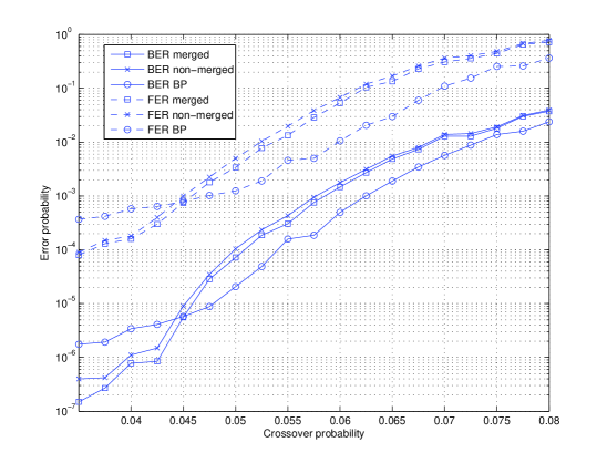
Figure 7: Simulation results for the BSC comparing the approximate LP decoder with and without merging of check nodes with belief propagation.

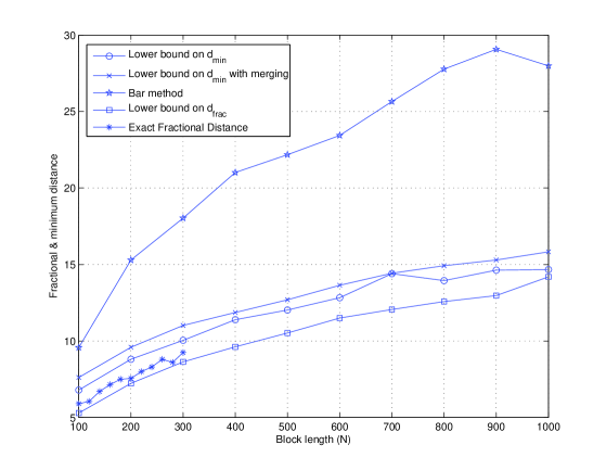
Figure 8: Lower bounds on the fractional distance and minimum distance.

VIII Numerical Results

In the experiments outlined below, Algorithm 1 was operated in the following mode, with respect to the values of the parameters $K$ and $\epsilon_{0}$. Initialize with $K=1000$ and $\epsilon_{0}=0.01$. Iterate until $\epsilon<\epsilon_{0}$. Then multiply $K$ by $1.26$, divide $\epsilon$ by $1.26$ and iterate with the new constraints. The process of iterating and multiplying and dividing by $1.26$ is repeated ten times, so that at the end of the process $K\approx 10000$ and $\epsilon_{0}\approx 0.001$.

Figure 7 shows simulation results comparing the approximate iterative LP decoder with and without merging of check nodes, as suggested in Section IV. In the simulation we picked codes at random from Gallager’s $(3,6)$-regular ensemble of length $N=1002$. These codes were transmitted over a binary symmetric channel. For the merging process, check nodes are picked as follows. First, a list of short cycles (up to maximum length of $6$) in the graph is generated using the procedure proposed in [19]. Based on this list, in each cycle we merge the check nodes into one new check node. This approach is motivated by Proposition 3, which guarantees an unchanged relaxation if the set of merged constraint nodes is cycle-free. As a reference, we also plot results for iterative belief propagation decoding. It is apparent from the figure that despite the improvement due to check node merging, the LP decoder exhibits worse performance than the belief propagation decoder for values of the channel crossover probability greater than $0.045$, and better performance for lower values of crossover probability.

In Figure 8, we plot our results from Sections V and VI. The lower bound on the minimum distance derived in Section V is shown in circles. This plot shows, for various block lengths, the average value of $\underline{l_{\min}}$ (see (49)) over $10$ randomly-generated codes, taken from Gallager’s $(3,4)$-regular ensemble. We also include improved bounds obtained by merging check nodes. Check nodes were chosen for merging as in Figure 7, using all cycles of length up to $6$.

Figure 8 also shows an improved lower bound on the minimum distance using the bar method outlined at the end of Section V. Clearly, in this case the lower bound is significantly improved by allowing pairs of nodes to be examined. Next, we plot the lower bound on the fractional distance from Section VI. The lower bound on the fractional distance is calculated with the penalty constant set to $B=10N$. In this case we set $\epsilon_{0}$ in Algorithm 1 to an initial value of $0.1/B$, instead of $0.01$ as previously stated; this more stringent setting was used in order to increase the accuracy of our result in light of the large value of $\gamma_{\max}$. Finally, exact fractional distance results, appearing in asterisks, are included in Figure 8. These results were taken from [1] and depict exact fractional distance, averaged over a sample of $100$ codes. With the exception of these exact results from [1], all results depict the average over the same $10$ randomly-generated codes, taken from Gallager’s $(3,4)$-regular ensemble. Comparing the exact results with our lower bound, we see that although the randomly-selected codes are not the same, the statistical averages indicate that the lower bound is close to the mark for $B=10N$.

IX Conclusion

In this paper we made obtained the following contributions to the framework of LP decoding. First, a method for improving LP decoding based on merging check nodes was proposed. Second, an algorithm for determining a lower bound on the minimum distance was presented. This algorithm can be improved by the check node merging technique or by the greedy procedure introduced in Section V. This algorithm has computation complexity $O(N^{2})$, where $N$ is the block length. Third, an algorithm for determining a tight lower bound on the minimum distance was presented. This algorithm also has complexity $O(N^{2})$. Fourth, we showed how the fundamental polytope can be obtained for GLDPC and nonbinary codes.

References

[1]
J. Feldman, M. J. Wainwright, and D. R. Karger,
“Using linear programming to decode binary linear codes,”
IEEE Transactions on Information Theory, vol. 51, no. 3, pp.
954–972, Mar 2005.
[2]
S. C. Draper, J. S. Yedidia, and Y. Wang,
“ML decoding via mixed-integer adaptive linear programming,”
in Proceedings of the IEEE International Symposium on
Information Theory (ISIT 2007), Nice, France, June 2007.
[3]
M. H. Taghavi and P. H. Siegel,
“Adaptive methods for linear programming decoding,”
IEEE Transactions on Information Theory, vol. 54, no. 12, pp.
5396–5410, December 2008.
[4]
A. G. Dimakis, A. A. Gohari, and M. J. Wainwright,
“Guessing facets: polytope structure and improved LP decoding,”
IEEE Transactions on Information Theory, vol. 55, no. 8, pp.
3479–3487, August 2009.
[5]
P. O. Vontobel and R. Koetter,
“Towards low-complexity linear-programming decoding,”
in Proc. 4th Int. Symposium on Turbo Codes and Related Topics,
Munich, Germany, April 2006,
arxiv:cs/0602088v1.
[6]
P. O. Vontobel and R. Koetter,
“On low-complexity linear-programming decoding of LDPC codes,”
European Transactions on Telecommunications, vol. 18, no. 5,
pp. 509–517, August 2007.
[7]
K. Yang, X. Wang, and J. Feldman,
“A new linear programming approach to decoding linear block
codes,”
IEEE Transactions on Information Theory, vol. 54, no. 3, pp.
1061–1072, Mar 2008.
[8]
D. Burshtein,
“Iterative approximate linear programming decoding of LDPC codes
with linear complexity,”
IEEE Transactions on Information Theory, vol. 55, no. 11, pp.
4835–4859, November 2009.
[9]
K. Fukuda and A. Prodon,
“Double Description Method Revisited,”
Report, ETHZ Zürich, Available:
ftp://ftp.ifor.math.ethz.ch/pub/fukuda/paper/ddrev960315.ps.gz, 1995.
[10]
T. S. Motzkin, H. Raiffa, G. L. Thompson, and R. M. Thrall,
“The double description method,”
Contributions to the theory of games, vol. 2, pp. 51– 73,
1953.
[11]
J.K. Wolf,
“Efficient maximum likelihood decoding of linear block codes using
a trellis,”
IEEE Transactions on Information Theory, vol. 24, no. 1, pp.
76–80, January 1978.
[12]
C. Hartmann and L. Rudolph,
“An optimum symbol-by-symbol decoding rule for linear codes,”
IEEE Transactions on Information Theory, vol. 22, no. 5, pp.
514–517, September 1976.
[13]
D. Bertsekas,
Convex Analysis and Optimization,
Athena Scientific, Belmont, Mass., 2003.
[14]
V. Skachek,
“Characterization of graph-cover pseudocodewords of codes over
,”
in Proceedings of the IEEE Information Theory Workshop (ITW
2010), Dublin, Ireland, September 2010.
[15]
M. F. Flanagan, V. Skachek, E. Byrne, and M. Greferath,
“Linear-programming decoding of nonbinary linear codes,”
IEEE Transactions on Information Theory, vol. 55, no. 9, pp.
4131–4154, September 2009.
[16]
G. L. Nemhauser and L. A. Wolsey,
Integer and Combinatorial Optimization,
Wiley, New York, 1988.
[17]
S. Boyd and L. Vandenberghe,
Convex Optimization,
Cambridge University Press, Cambridge, UK, 2004.
[18]
K. Fukuda,
“CDD and CDD+ homepage,”
http://www.ifor.math.ethz.ch/fukuda/cddhome/cdd.html,
2008.
[19]
James C. Tiernan,
“An efficient search algorithm to find the elementary circuits of a
graph,”
Commun. ACM, vol. 13, no. 12, pp. 722–726, 1970.