Role of Chameleon Field in Accelerating Universe

Abstract

In this work, we have considered a model of the flat FRW universe filled with cold dark matter and Chameleon field where the scale function is taken as, (i) Intermediate Expansion and (ii) Logamediate Expansion. In the both cases we find the expressions of Chameleon field, Chameleon potential, statefinder parameters and slow-roll parameters. Also it has been shown that the potential is always decreases with the chameleon field in both the scenarios. The nature of slow-roll parameters have been shown diagrammatically.

I Introduction

Dark energy is the mysterious entity that accounts for $70\%$ of the mass-energy content of the universe and is causing the expansion of the universe to accelerate. The current cosmological observations [1-3] and theories suggest that the Universe is undergoing an accelerated expansion due to dark energy. Possible candidates for this dark energy are a cosmological constant, a slowly rolling scalar field, Chaplygin gas, Tachyonic field etc. The cosmological constant scenario with a spatially flat or a nearly spatially flat Universe implies an energy density of order $\rho_{critical}=3H_{0}^{2}/8\pi G$ today. In this model, this energy density should be constant in time, giving rise to severe problems (see ref.[4]), making the explanation of dark energy with a cosmological constant which is unnatural. A more general model is that of a slowly rolling scalar field, known as quintessence, which has a negative pressure and therefore accelerates expansion.

Researchers at Fermilab in the US have carried out the first laboratory experiment to look for a hypothetical form of matter known as Chameleon Particles. Chameleon particles were first proposed in 2003 by Justin Khoury and Amanda Weltman [5] at Columbia University as a possible explanation for dark energy. In places where the density of matter is relatively high, chameleon particles interact very weakly with other matter and only over very short distances, which could explain why we have yet to spot them here on Earth. In the inter-galactic space where matter density is extremely low, the particles interact much more strongly with other matter and over very large distances. The particles could be spotted by how they affect light travelling to Earth from distant galaxies which are considered details in ref. [6-8].

If chameleon particles could be created within a steel-walled vacuum chamber of few centimeters in diameter and several meters long(which is called GammaV Chamber), many of them would be unable to escape, that is because the mass of a chameleon is proportional to the local density. Chameleons be created by firing a laser into a region of the chamber containing a very high magnetic field. If the chameleon field couples strongly to matter, we would have already detected it as a fifth force in gravitational experiments. A candidate one could come up with for such a scalar field could be the dilation from string theory. There exists a mechanism which suppresses the coupling of the field to matter, avoiding detection. Recently, a new model was suggested [5] such that: in which a scalar field with a thin-shell mechanism couples to matter with gravitational strength while remaining very light on cosmological scales. The crucial feature of this field is that the coupling gives it a mass depending on the local density of matter. Thus the scalar field is named chameleon. Several works has been done due to Chameleon field [9-13]. In regions of high matter density, chameleon field has a large mass and therefore its interaction with matter is small. In regions of low energy density, like the solar system, the mass is small and the interaction should be large and observable. The action of this field is suppressed by a so called thin-shell mechanism, to be discussed later. In opposition to slow rolling scalar field models, chameleons are not limited to quintessence.

The paper is organized as follows: In section II, we have considered a flat FRW model which represents the corresponding equation of Chameleon Field where the scale function is taken as, (i) Intermediate Expansion and (ii) Logamediate Expansion. In both the cases we find the expressions of the Chameleon field, Chameleon potential and slow-roll parameters. We have taken some particular values of the parameters and constants for the graphical representation. The paper ends with a short discussion in section III.

II Basic Equations for the Chameleon Field

The metric of a spatially flat isotropic and homogeneous Universe in FRW model is,

$$ds^{2}=dt^{2}-a^{2}(t)\left[dr^{2}+r^{2}(d\theta^{2}+sin^{2}\theta d\phi^{2})\right]$$ (1)

where $a(t)$ is the scale factor of the universe. The Hubble parameter is defined as,

$$H=\frac{\dot{a}}{a}$$ (2)

Consider the relevant action is given by,

$$S=\int\sqrt{-g}d^{4}x[f(\phi){\cal L}+\frac{1}{2}\phi_{,\mu}\phi^{,\mu}+\frac{\cal{R}}{16\pi G}-V(\phi)]$$ (3)

where, $\phi$ is the Chameleon Scalar Field and $V(\phi)$ is the Chameleon potential. Also, ${\cal{R}}$ is the Ricci Scalar, $G$ is the Newtonian constant of gravity. $f(\phi){\cal L}$ is the modified Lagrangian matter and $f(\phi)$ is an analytic function of $\phi$. The cold dark matter and chameleon field interact with each other. The variation of action of the above equation w.r.t $\phi$ gives,

$$3H\dot{\phi}+\ddot{\phi}+\frac{dV}{d\phi}+(p+\rho)\frac{df}{d\phi}=0$$ (4)

which reduces to,

$$3H\dot{\phi}^{2}+\dot{\phi}\ddot{\phi}+\dot{V}+(p+\rho)\dot{f}=0$$ (5)

which is the wave equation for the chameleon field. Again, the variation of the same equation w.r.t. metric tensor components gives (choosing $8\pi G=1$),

$$3\frac{\dot{a}^{2}}{a^{2}}=\rho f+\frac{1}{2}\dot{\phi}^{2}+V(\phi)$$ (6)

and

$$2\frac{\ddot{a}}{a}+\frac{\dot{a}^{2}}{a^{2}}=-pf-\frac{1}{2}\dot{\phi}^{2}+V(\phi)$$ (7)

which are the corresponding field equations. For simplifying the above model we consider,

$$V=V_{0}\dot{\phi}^{2}$$ (8)

where, $V_{0}$ is a constant, $p$ is the pressure and $\rho$ is the energy density. Now, combining equations (5), (6) and (7), we get,

$$\frac{\partial}{\partial t}(\rho f)+3H(p+\rho)f=(p+\rho)\dot{f}$$ (9)

Simplifying the above equation we get,

$$\frac{d\rho}{p}+3\frac{da}{a}\left(1+\frac{\rho}{p}\right)=\frac{df}{f}$$ (10)

To get a complete solution of the above differential equation, we consider the barotropic equation of state

$$p=\omega\rho$$ (11)

where $\omega$ is a constant. Equations (9) and (11) together gives,

$$\rho=\rho_{0}a^{-3(1+\omega)}f^{\omega}$$ (12)

where $\rho_{0}$ is the integrating constant. If $\omega=0$, then from (11) and (12) we get,

$$p=0~{}~{}~{}and~{}~{}~{}\rho=\rho_{0}/a^{3}$$ (13)

this is the case where a particular matter dominated the universe and then the fluid is taken in the form of pressureless dust which is considered in ref [12].

II.1 Chameleon Field in case of Intermediate Inflation

Consider a particular scenario of Intermediate Inflation [14], where the scale factor $a(t)$ of the Friedmann universe is described as,

$$a(t)=\exp(Bt^{\beta})$$ (14)

where $B\beta>0$, $B>0$ and $0<\beta<1$ are constants. The Hubble parameter becomes,

$$H=\frac{\dot{a}}{a}=B\beta t^{\beta-1}$$ (15)

In this case the expansion of Universe is faster than Power-Law Inflation, where the scale factor is given as, $a(t)=t^{n}$, where $n>1$ is a constant. Also, the expansion of the Universe is slower for Standard De Sitter Inflation where $\beta=1$. Hence we get,

$$\frac{\dot{H}}{H}=\frac{\beta-1}{t}$$ (16)

$$\frac{\ddot{H}}{H}=\frac{(\beta-1)(\beta-2)}{t^{2}}$$ (17)

and

$$\frac{\ddot{a}}{a}=B^{2}\beta^{2}t^{2\beta-2}+B\beta(\beta-1)t^{\beta-2}$$ (18)

Putting the value of $a(t)$ the declaration parameter $q=-\frac{a{\ddot{a}}}{{\dot{a}}^{2}}$ we get,

$$q=-1-\frac{\beta-1}{B\beta t^{\beta}}$$ (19)

Fig.1 represents the variation of $q$ against $H$ for different values of $\beta$.

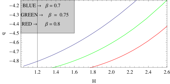
Figure 1: The variation of $q$ against $H$ from eq. (19) for $B=3$,$\omega=.2$,$V_{0}$=2 and $\beta=0.7,0.75,0.8$

The flat Friedmann model which is analyzed in terms of the statefinder parameters. The trajectories in the $\{s,r\}$ plane of different cosmological models shows different behavior. The statefinder diagnostic of SNAP observations used to discriminate between different dark energy models. The statefinder diagnostic pair is constructed from the scale factor $a(t)$. The statefinder diagnostic pair is denoted as $\{s,r\}$ and defined as [15],

$$r=\frac{\dddot{a}}{aH^{3}}~{}~{}~{}\text{and}~{}~{}~{}s=\frac{r-1}{3(q-\frac{1}{2})}$$ (20)

Using (15) and (19), equation (20) becomes,

$$r=1+\frac{(\beta-1)(\beta-2)}{B^{2}\beta^{2}}t^{-2\beta}+\frac{\beta+1}{B\beta}t^{-\beta}$$ (21)

and

$$s=-\frac{\frac{(\beta-1)(\beta-2)}{B\beta t^{\beta}}+\beta+1}{3(\beta-1)+\frac{9B\beta t^{\beta}}{2}}$$ (22)

Fig.2 represents the variation of $s$ against $r$ for different values of $\beta$.

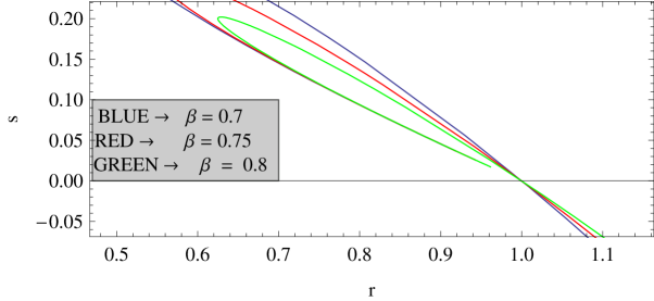
Figure 2: The variation of $s$ against $r$ from (21) and (22) for $B=3$,$\omega=.2$,$V_{0}$=2 and $\beta=0.7,0.75,0.8$

Using (8), (11) and (14), equations (6) and (7) become

$$3B^{2}\beta^{2}t^{2\beta-2}=\rho f+\frac{2V_{0}+1}{2}\dot{\phi}^{2}$$ (23)

and

$$2B^{2}\beta^{2}t^{2\beta-2}+2B\beta(\beta-1)t^{\beta-2}+B^{2}\beta^{2}t^{2\beta-2}=-\rho\omega f+\frac{2V_{0}-1}{2}\dot{\phi}^{2}$$ (24)

Eliminating $f$ from (23) and (24) we get,

$$3B^{2}\beta^{2}(\omega+1)t^{2\beta-2}+2B\beta(\beta-1)t^{\beta-2}=\frac{2(\omega+1)V_{0}+(\omega-1)}{2}\dot{\phi}^{2}$$ (25)

Thus using (8) and (25) we get the Chameleon Field and Chameleon Potential as,

$$\phi=\int\sqrt{\frac{3B^{2}\beta^{2}(\omega+1)t^{2\beta-2}+2B\beta(\beta-1)t^{\beta-2}}{(\omega+1)V_{0}+\frac{\omega-1}{2}}}dt$$ (26)

and

$$V(\phi)=\frac{3B^{2}\beta^{2}(\omega+1)t^{2\beta-2}+2B\beta(\beta-1)t^{\beta-2}}{\omega+1+\frac{\omega-1}{2V_{0}}}$$ (27)

Fig.3  represents the variation of $V$ against $\phi$ for different values of $\beta$. It has been seen that the potential is always decreases with the chameleon field $\phi$.

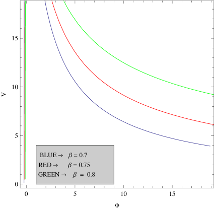
Figure 3: The variation of $V$ against $\phi$ from (26) and (27) for $B=3$,$\omega=0.2$,$V_{0}$=2 and $\beta=0.7,0.75,0.8$

The slow-roll parameters are defined as [14],

$$\epsilon=2\left(\frac{H^{\prime}}{H}\right)^{2}=\frac{2{\dot{H}}^{2}}{H^{2}\phi^{2}}$$ (28)

and

$$\eta=\frac{2H^{\prime\prime}}{H}=\frac{2}{H}\left(\frac{\ddot{H}}{\dot{\phi}^{2}}-\frac{\dot{H}\ddot{\phi}}{\dot{\phi}^{3}}\right)$$ (29)

From (26) we get,

$$\dot{\phi}^{2}=\frac{3B^{2}\beta^{2}(\omega+1)t^{2\beta-2}+2B\beta(\beta-1)t^{\beta-2}}{(\omega+1)V_{0}+\frac{\omega-1}{2}}$$ (30)

Differentiate the above equation w.r.t. $t$ we get,

$$\dot{\phi}\ddot{\phi}=\frac{3B^{2}\beta^{2}(\beta-1)(\omega+1)t^{2\beta-3}+B\beta(\beta-1)(\beta-2)t^{\beta-3}}{(\omega+1)V_{0}+\frac{\omega-1}{2}}$$ (31)

In this case using (16), (17), (28), (29), (30) and (31) we get,

$$\epsilon=\frac{2(\beta-1)^{2}((\omega+1)V_{0}+\frac{\omega-1}{2})}{3B^{2}\beta^{2}(\omega+1)t^{2\beta}+2B\beta(\beta-1)t^{\beta}}$$ (32)

and

$$\eta=\frac{(\beta-1)(\beta-2)(2(\omega+1)V_{0}+\omega-1)}{B\beta t^{\beta}(3B\beta(\omega+1)t^{\beta}+2\beta-2)}-\frac{(\beta-1)^{2}(2(\omega+1)V_{0}+\omega-1)(3B\beta(\omega+1)t^{\beta}+\beta-2)}{B\beta t^{\beta}(3B\beta(\omega+1)t^{\beta}+2\beta-2)^{2}}$$ (33)

Fig.4  represents the variation of $\eta$ against $\epsilon$ for different values of $\beta$. From the figure, it has been seen that $\eta$ decreases with $\epsilon$ with $\eta$ is always positive and $\epsilon$ is always negative.

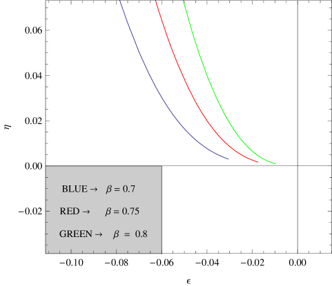
Figure 4: The variation of $\eta$ against $\epsilon$ from (32) and (33) for $B=3$,$\omega$=0.2,$V_{0}$=2 and $\beta$=0.7,0.75,0.8

Thus from (12) and (14) the energy density becomes.

$$\rho=\rho_{0}a^{-3(1+\omega)}f^{\omega}=\rho_{0}\exp(-3B(1+\omega)t^{\beta})f^{\omega}$$ (34)

From (11) and (32) the pressure becomes,

$$p=\rho_{0}\omega a^{-3(1+\omega)}f^{\omega}=\rho_{0}\omega\exp(-3B(1+\omega)t^{\beta})f^{\omega}$$ (35)

Now from (5), (8), (15), (32) and (33) we have,

$$(2V_{0}+1)\dot{\phi}\ddot{\phi}+3B\beta t^{\beta-1}\dot{\phi}^{2}=-\rho_{0}(1+\omega)\exp(-3B(1+\omega)t^{\beta})f^{\omega}\dot{f}$$ (36)

So, equation (34), (35) and (36) together gives,

$$\rho_{0}(1+\omega)f^{\omega}\dot{f}=-\frac{\exp(3B(1+\omega)t^{\beta})}{(\omega+1)V_{0}+\frac{\omega-1}{2}}\times$$

$$[B\beta t^{\beta-3}(\beta-1)(2V_{0}+1)(3B\beta(\omega+1)t^{\beta}+\beta-2)+3B^{2}\beta^{2}t^{2\beta-3}(3B\beta(\omega+1)t^{\beta}+2\beta-2)]$$ (37)

Integrating both sides of the above equation w.r.t. $t$ and after a further calculation we obtain,

$$f=\left[-\int\left\{\frac{\exp(3B(1+\omega)t^{\beta})}{(\omega+1)V_{0}+\frac{\omega-1}{2}}\times\frac{x}{\rho_{0}}\right\}~{}dt\right]^{\frac{1}{1+\omega}}$$ (38)

where, $x=B\beta t^{\beta-3}(\beta-1)(2V_{0}+1)(3B\beta(\omega+1)t^{\beta}+\beta-2)+3B^{2}\beta^{2}t^{2\beta-3}(3B\beta(\omega+1)t^{\beta}+2\beta-2)$.

So from equation (32), (33) and (38) we get the expressions of energy density and pressure as

$$\rho=\rho_{0}\exp(-3B\beta(1+\omega)t^{\beta})\left[-\int\frac{\exp(3B(1+\omega)t^{\beta})}{(\omega+1)V_{0}+\frac{\omega-1}{2}}\times\frac{x}{\rho_{0}}~{}dt\right]^{\frac{\omega}{1+\omega}}$$ (39)

and

$$p=\rho_{0}\omega\exp(-3B\beta(1+\omega)t^{\beta})\left[-\int\frac{\exp(3B(1+\omega)t^{\beta})}{(\omega+1)V_{0}+\frac{\omega-1}{2}}\times\frac{x}{\rho_{0}}~{}dt\right]^{\frac{\omega}{1+\omega}}$$ (40)

II.2 Chameleon Field in case of Logamediate Inflation:-

Consider a particular scenario of Logamediate Inflation [14], where the scale factor $a(t)$ is described as,

$$a(t)=\exp(A(\ln t)^{\alpha})$$ (41)

where $A\alpha>0$ and $\alpha>1$. The Hubble parameter $H=\frac{\dot{a}}{a}$ becomes,

$$H=\frac{A\alpha}{t}(\ln t)^{\alpha-1}$$ (42)

Hence from (42) we get,

$$\frac{\dot{H}}{H}=\frac{\alpha-1-\ln t}{t\ln t}$$ (43)

and

$$\frac{\ddot{H}}{H}=\frac{2(\ln t)^{2}-3(\alpha-1)\ln t+(\alpha-1)(\alpha-2)}{t^{2}(\ln t)^{2}}$$ (44)

From (41) we get,

$$\frac{\ddot{a}}{a}=\frac{A^{2}\alpha^{2}}{t^{2}}(\ln{t})^{2\alpha-2}-\frac{A\alpha}{t^{2}}(\ln{t}-\alpha+1)(\ln{t})^{\alpha-2}$$ (45)

Putting the value of $a(t)$ the declaration parameter $q=-\frac{a\ddot{a}}{\dot{a}^{2}}$ we get,

$$q=-1+\frac{\ln t-\alpha+1}{A\alpha(\ln{t})^{\alpha}}$$ (46)

Fig.5 represents the variation of $q$ against $H$ for different values of $\alpha$.

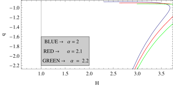
Figure 5: The variation of $q$ against $H$ from (46) for $A=1$,$\omega=.2$,$V_{0}$=2 and $\alpha=2,2.1,2.2$

From (20), (41), (42) and (46) we get the expressions for the statefinder parameters as

$$r=1+\frac{3(\alpha-1)}{A\alpha(\ln{t})^{\alpha}}-\frac{3}{A\alpha(\ln{t})^{\alpha-1}}+\frac{2}{A^{2}\alpha^{2}(\ln{t})^{2\alpha-2}}-\frac{3(\alpha-1)}{A^{2}\alpha^{2}(\ln{t})^{2\alpha-1}}+\frac{(\alpha-1)(\alpha-2)}{A^{2}\alpha^{2}(\ln{t})^{2\alpha}}$$ (47)

and

$$s=\frac{\frac{3(\alpha-1)}{A\alpha(\ln{t})^{\alpha}}-\frac{3}{A\alpha(\ln{t})^{\alpha-1}}+\frac{2}{A^{2}\alpha^{2}(\ln{t})^{2\alpha-2}}-\frac{3(\alpha-1)}{A^{2}\alpha^{2}(\ln{t})^{2\alpha-1}}+\frac{(\alpha-1)(\alpha-2)}{A^{2}\alpha^{2}(\ln{t})^{2\alpha}}}{\frac{3}{A\alpha(\ln{t})^{\alpha-1}}-\frac{3(\alpha-1)}{A\alpha(\ln{t})^{\alpha}}-\frac{9}{2}}$$ (48)

Fig.6 represents the variation of $s$ against $r$ for different values of $\alpha$.

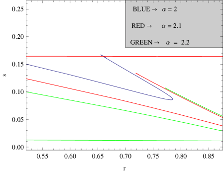
Figure 6: The variation of $s$ against $r$ from (47) and (48) for $A=1$,$\omega=.2$,$V_{0}$=2 and $\alpha=2,2.1,2.2$

From equation (6), (7), (8), (11), (42) and (45) we get,

$$2\left\{\frac{A^{2}\alpha^{2}}{t^{2}}(\ln{t})^{2\alpha-2}-\frac{A\alpha}{t^{2}}(\ln{t}-\alpha+1)(\ln{t})^{\alpha-2}\right\}+(3\omega+1)\left\{\frac{A\alpha}{t}(\ln t)^{\alpha-1}\right\}^{2}=\dot{\phi}^{2}\left[V_{0}(\omega+1)+\frac{1}{2}(\omega-1)\right]$$ (49)

Thus using (8) and (49) we get the Chameleon Field and Chameleon Potential as,

$$\phi=\int\sqrt{\frac{3A^{2}\alpha^{2}(\omega+1)(\ln{t})^{2\alpha-2}-2A\alpha(\ln{t}-\alpha+1)(\ln{t})^{\alpha-2}}{(\omega+1)V_{0}+\frac{\omega-1}{2}}}~{}\cdot~{}\frac{dt}{t}$$ (50)

and

$$V(\phi)=\frac{V_{0}}{t^{2}}\times\frac{3A^{2}\alpha^{2}(\omega+1)(\ln{t})^{2\alpha-2}-2A\alpha(\ln{t}-\alpha+1)(\ln{t})^{\alpha-2}}{(\omega+1)V_{0}+\frac{\omega-1}{2}}$$ (51)

Fig.7  represents the variation of $V$ against $\phi$ for different values of $A$ and $\alpha$.

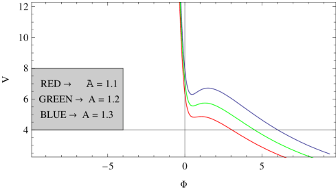
Figure 7: The variation of $V$ against $\phi$ from (50) and (51) for $A=1.1,1.2,1.3$,  $\omega=0.2$,$V_{0}$=2 and $\alpha=2$

From (28), (29), (43), (44) and (50) we get the slow-roll parameters,

$$\epsilon=\frac{2(\ln{t}-\alpha+1)^{2}\times((\omega+1)V_{0}+\frac{\omega-1}{2})}{3A^{2}\alpha^{2}(\omega+1)(\ln{t})^{2\alpha}-2A\alpha(\ln{t}-\alpha+1)(\ln{t})^{\alpha}}$$ (52)

and

$$\eta=\frac{(2V_{0}(\omega+1)+\omega-1)\times(2(\ln t)^{2}-3(\alpha-1)\ln{t}+(\alpha-1)(\alpha-2))}{3A^{2}\alpha^{2}(\omega+1)(\ln{t})^{2\alpha}-2A\alpha(\ln{t}-\alpha+1)(\ln{t})^{\alpha}}+\frac{((\omega+1)V_{0}+\frac{\omega-1}{2})(\ln t-\alpha+1)}{A\alpha(\ln t)^{\alpha-2}}\times$$

$$\frac{-3A\alpha(\omega+1)(\ln{t}-\alpha+1)(\ln{t})^{\alpha}+(2(\ln t)^{2}-3(\alpha-1)\ln{t}+(\alpha-1)(\alpha-2))}{[3A\alpha(\omega+1)(\ln t)^{\alpha}-2(\ln t-\alpha+1)]^{2}}$$ (53)

Fig.8  represents the variation of $\eta$ against $\epsilon$ for different values of $\alpha$. It has been seen that $\eta$ is decreases with $\epsilon$.

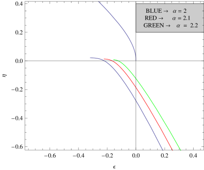
Figure 8: The variation of $\eta$ against $\epsilon$ from (52) and (53) for $A=1$,$\omega$=0.2,$V_{0}$=2 and $\alpha$=2,2.1,2.2

Thus from (11), (12) and (41) the energy density and pressure becomes.

$$\rho=\rho_{0}a^{-3(1+\omega)}f^{\omega}=\rho_{0}\exp(-3A(1+\omega)(\ln{t})^{\alpha})f^{\omega}$$ (54)

and

$$p=\rho_{0}\omega a^{-3(1+\omega)}f^{\omega}=\rho_{0}\omega\exp(-3A(1+\omega)(\ln{t})^{\alpha})f^{\omega}$$ (55)

Now from (5), (8), (42), (54) and (55) we have,

$$(2V_{0}+1)\dot{\phi}\ddot{\phi}+\frac{3A\alpha}{t}(\ln{t})^{\alpha-1}\dot{\phi}^{2}=-\rho_{0}(1+\omega)\exp(-3A(1+\omega)(\ln{t})^{\alpha}))f^{\omega}\dot{f}$$ (56)

From (50) we get,

$${\dot{\phi}}^{2}=\frac{3A^{2}\alpha^{2}(\omega+1)(\ln{t})^{2\alpha-2}-2A\alpha(\ln{t}-\alpha+1)(\ln{t})^{\alpha-2}}{t^{2}((\omega+1)V_{0}+\frac{\omega-1}{2})}$$ (57)

Differentiate the above equation w.r.t. $t$ we get,

$$\dot{\phi}\ddot{\phi}=\frac{A\alpha(\ln t)^{\alpha-3}}{((\omega+1)V_{0}+\frac{\omega-1}{2})t^{3}}[-3A\alpha(\omega+1)(\ln{t}-\alpha+1)(\ln{t})^{\alpha}+(2(\ln t)^{2}-3(\alpha-1)\ln{t}+(\alpha-1)(\alpha-2))]$$ (58)

So, equations (5), (8), (11), (57) and (58) together give,

$$\rho_{0}(1+\omega)f^{\omega}\dot{f}\exp(-3A(1+\omega)(\ln{t})^{\alpha})=-\frac{3A^{2}\alpha^{2}(\ln t)^{2\alpha-3}}{((\omega+1)V_{0}+\frac{\omega-1}{2})t^{3}}[3A\alpha(\omega+1)(\ln t)\alpha-2(\ln t-\alpha+1)]$$

$$-\frac{(2V_{0}+1)A\alpha(\ln t)^{\alpha-3}}{((\omega+1)V_{0}+\frac{\omega-1}{2})t^{3}}[-3A\alpha(\omega+1)(\ln{t}-\alpha+1)(\ln{t})^{\alpha}+(2(\ln t)^{2}-3(\alpha-1)\ln{t}+(\alpha-1)(\alpha-2))]$$ (59)

Assume, $X(t)=-\frac{3A^{2}\alpha^{2}(\ln t)^{2\alpha-3}}{((\omega+1)V_{0}+\frac{\omega-1}{2})t^{3}}[3A\alpha(\omega+1)(\ln t)\alpha-2(\ln t-\alpha+1)]$
and $Y(t)=-\frac{(2V_{0}+1)A\alpha(\ln t)^{\alpha-3}}{((\omega+1)V_{0}+\frac{\omega-1}{2})t^{3}}[-3A\alpha(\omega+1)(\ln{t}-\alpha+1)(\ln{t})^{\alpha}+(2(\ln t)^{2}-3(\alpha-1)\ln{t}+(\alpha-1)(\alpha-2))]$

Integrating both sides of the above equation w.r.t. $t$ and after a further calculation we obtain

$$f=\left[\frac{1}{\rho_{0}}\int{\exp(3A(1+\omega)(\ln{t})^{\alpha})(X(t)+Y(t))}dt\right]^{\frac{1}{1+\omega}}$$ (60)

So from equations (54), (55) and (60) we get the expressions of the energy density and pressure as

$$\rho=\rho_{0}\exp(-3A(1+\omega)(\ln{t})^{\alpha})\left[\frac{1}{\rho_{0}}\int{\exp(3A(1+\omega)(\ln{t})^{\alpha})(X(t)+Y(t))}dt\right]^{\frac{\omega}{1+\omega}}$$ (61)

and

$$p=\rho_{0}\omega\exp(-3A(1+\omega)(\ln{t})^{\alpha})\left[\frac{1}{\rho_{0}}\int{\exp(3A(1+\omega)(\ln{t})^{\alpha})(X(t)+Y(t))}dt\right]^{\frac{\omega}{1+\omega}}$$ (62)

III Discussions

In this work, we have considered a model of the flat FRW universe filled with cold dark matter and Chameleon field where the scale function is taken as, (i) Intermediate Expansion and (ii) Logamediate Expansion. In the both cases we find the expressions of Chameleon field, Chameleon potential, statefinder parameters and slow-roll parameters. In both the cases, it has been shown that the potential is always decreases with the chameleon field. From figures, we have seen the nature of slow-roll parameters i.e., $\eta$ is always decreasing with $\epsilon$. We have taken some particular values of the parameters and constants for the graphical representation. In both the cases, we have found the expressions of $f$, energy density and pressure of the cold dark matter in terms of cosmic time $t$.

References:

$[1]$ N. A. Bachall, J. P. Ostriker, S. Perlmutter and P. J. Steinhardt, Science 284 1481 (1999).
$[2]$ S. J. Perlmutter et al, Astrophys. J. 517 565 (1999).
$[3]$ A. G. Riess et al, Astron. J. 116 1009 (1998).
$[4]$ P. Brax and J. Martin, astro-ph/0210533.
$[5]$ J. Khoury and A. Weltman, Phys. Rev. Lett. 93 171104 (2004); arXiv:astro-ph/0309300.
$[6]$ S. Perlmutter et al., Bull. Am. Astron. Soc. 29 1351 (1997).
$[7]$ J. L. Tonry et al., Astrophys. J. 594 1 (2003).
$[8]$ S. Bridle, O. Lahav, J. P. Ostriker and P. J. Steinhardt, Science 299 1532 (2003).
$[9]$ P. Brax, C. van de Bruck, A. C. Davis, J. Khoury and A. Weltman, AIP Conf. Proc. 736 105 (2005); astro-ph/0410103.
$[10]$ H. Wei and R. -G. Cai, Phys. Rev. D 71 043504 (2005).
$[11]$ D. F. Mota and D. J. Shaw, Phys. Rev. Lett. 97 151102 (2006).
$[12]$ N. Banerjee, S. Das and K. Ganguly, arXiv:0801.1204v1[gr-qc].
$[13]$ N. Banerjee and S. Das, Phys. Rev. D 78 043512 (2008).
$[14]$ J. D. Barrow and N. J. Nunes, Phys. Rev. D 76 043501 (2007).
$[15]$ V. Sahni, T. D. Saini, A. A. Starobinsky and U. Alam, JETP Lett. 77 201 (2003).