Dynamics of Logamediate and Intermediate Scenarios in the Dark Energy Filled Universe

Abstract

We have considered a model of two component mixture i.e., mixture of Chaplygin gas and barotropic fluid with tachyonic field. In the case, when they have no interaction then both of them retain their own properties. Let us consider an energy flow between barotropic and tachyonic fluids. In both the cases we find the exact solutions for the tachyonic field and the tachyonic potential and show that the tachyonic potential follows the asymptotic behavior. We have considered an interaction between these two fluids by introducing a coupling term. Finally, we have considered a model of three component mixture i.e., mixture of tachyonic field, Chaplygin gas and barotropic fluid with or without interaction. The coupling functions decays with time indicating a strong energy flow at the initial period and weak stable interaction at later stage. To keep the observational support of recent acceleration we have considered two particular forms (i) Logamediate Scenario and (ii) Intermediate Scenario, of evolution of the Universe. We have examined the natures of the recent developed statefinder parameters and slow-roll parameters in both scenarios with and without interactions in whole evolution of the universe.

I Introduction

Recent observations of the luminosity of type Ia supernovae indicate [1-7] an accelerated expansion of the universe and lead to the search for a new type of matter which violate the strong energy condition $\rho+3p<0$. The matter consent responsible for such a condition to be satisfied at a certain stage of evolution of the universe is referred to as dark energy. There are different candidates to play the role of the dark energy. The type of dark energy represented by a scalar field is often called Quintessence. The transition from a universe filled with matter to an exponentially expanding universe does not necessarily require the presence of the scalar field as the only alternative. In particular one can try another alternative by using an exotic type of fluid - the so-called Chaplygin gas [8-14]. Assume that the cosmological model, which is denoted by $\Lambda$CDM, contains a cosmological constant $\Lambda$ and the cold dark matter. In the presence of an interaction the dark energy can achieve a stable equilibrium that differs from the usual de Sitter case. The effective equations of state of matter and dark energy coincide and behave like cold dark matter (CDM) at early times. Actually, dark energy is a mysterious fluid, contains enough negative pressure causes the present day acceleration.

The energy-momentum tensor of the tachyonic field [15] can be seen as a combination of two fluids, dust with pressure zero and a cosmological constant with $p=-\rho$, thus generating enough negative pressure such as to drive acceleration. Also the tachyonic field has a potential which has an unstable maximum at the origin and decays to almost zero as the field goes to infinity. Depending on various forms of this potential following this asymptotic behaviour a lot of works have been carried out on tachyonic dark energy [16-19], tachyonic dark matter [20-22] and inflation models [23,24].

Here we consider a model of two component mixture i.e., mixture of Chaplygin gas and barotropic fluid with tachyonic field. In the case, when they have no interaction then both of them retain their own properties. Let us consider an energy flow between barotropic and tachyonic fluids. In both the cases we find the exact solutions for the tachyonic field and the tachyonic potential and show that the tachyonic potential follows the asymptotic behavior. Later we have also considered an interaction between these two fluids by introducing a coupling term. The coupling function decays with time indicating a strong energy flow at the initial period and weak stable interaction at later stage. To keep the observational support of recent acceleration we have considered two particular forms: (i) Logamediate Scenario [25] and (ii) Intermediate Scenario[25, 26], of evolution of the Universe. The intermediate and logamediate Scenarios are motivated by considering a class of possible cosmological solutions with indefinite expansion which result from imposing weak general conditions on the cosmological model. The intermediate Scenario satisfies the bounds on the spectral index $n_{s}$ and ratio of tensor-to-scalar perturbations, $r$, as measured by the latest observations of the CMB. For observationally viable models of logamediate Scenario, the ratio of tensor-to-scalar perturbations, $r$, must be small and that the power spectrum can be either red or blue tilted, depending on the specific parameters of the model. It has the interesting property that the cooperative evolution We have examined the nature of the recent developed statefinder parameters [27] and slow-roll parameters [25] in whole evolution of the universe.

The paper is organized as follows: Section II deals with the field equations of the tachyonic field in logamediate and intermediate scenarios of the universe. In sections III we have considered models represented by mixture of tachyonic field with GCG. In sections IV we have considered models represented by mixture of tachyonic field with barotropic fluid. In sections V we have considered models represented by mixture of tachyonic field with GCG and Barotropic fluid. These three sections are each subdivided into two parts showing the effect of these models with or without interaction. We have found also the expressions of slow-roll-parameter. We have taken some particular values of the parameters and constants for the graphical representation. The paper ends with a short discussion in section VI.

II Einstein Field Equations and Tachyonic Fluid Model

The metric of a spatially flat isotropic and homogeneous Universe in FRW model is

$$ds^{2}=dt^{2}-a^{2}(t)\left[dr^{2}+r^{2}(d\theta^{2}+sin^{2}\theta d\phi^{2})\right]$$ (1)

where $a(t)$ is the scale factor of the universe. The Einstein field equations are (choosing $8\pi G=c=1$)

$$3H^{2}=\rho_{tot}$$ (2)

and

$$6(\dot{H}+H^{2})=-(\rho_{tot}+p_{tot})$$ (3)

where, $\rho_{tot}$ and $p_{tot}$ are respectively the total energy density and the pressure of the Universe. Here $H$ is called Hubble parameter defined as,

$$H=\frac{\dot{a}}{a}$$ (4)

In the following, we’ll discuss the natures of statefinder parameters and deceleration parameter in the particular forms of logamediate and intermediate Scenario.

II.1 Logamediate Scenario

Consider a particular form of Logamediate Scenario [25], where the form of the scale factor $a(t)$ is defined as,

$$a(t)=\exp(A(\ln t)^{\alpha})$$ (5)

where $A\alpha>0$ and $\alpha>1$. When $\alpha=1$, this model reduces to power-law form. The logamediate form is motivated by considering a class of possible cosmological solutions with indefinite expansion which result from imposing weak general conditions on the cosmological model. Barrow [25] has found in their model, the observational ranges of the parameters are as follows: $1.5\times 10^{-92}\leq A\leq 2.1\times 10^{-2}$ and $2\leq\alpha\leq 50$. The Hubble parameter $H=\frac{\dot{a}}{a}$ becomes,

$$H=\frac{A\alpha}{t}(\ln t)^{\alpha-1}$$ (6)

Hence from (6) we get,

$$\frac{\dot{H}}{H}=\frac{\alpha-1-\ln t}{t\ln t}$$ (7)

and

$$\frac{\ddot{H}}{H}=\frac{2(\ln t)^{2}-3(\alpha-1)\ln t+(\alpha-1)(\alpha-2)}{t^{2}(\ln t)^{2}}$$ (8)

Putting the value of $a(t)$ in the deceleration parameter $q=-\frac{a\ddot{a}}{\dot{a}^{2}}$ we get,

$$q=-1+\frac{\ln t-\alpha+1}{A\alpha(\ln{t})^{\alpha}}$$ (9)

where $a(t)$ is the scale factor. Fig.1 represents the variation of $H$ against $q$ for different values of $\alpha$.

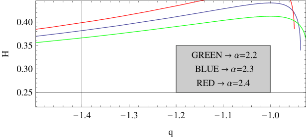
Figure 1: The variation of $H$ against $q$ for logamediate Scenario with $A=1$ and $\alpha=2.2,2.3,2.4$

The flat Friedmann model which is analyzed in terms of the statefinder parameters. The trajectories in the $\{s,r\}$ plane of different cosmological models shows different behavior. The statefinder diagnostic of SNAP observations used to discriminate between different dark energy models. The statefinder diagnostic pair is constructed from the scale factor $a(t)$. The statefinder diagnostic pair is denoted as $\{s,r\}$ and defined as [27],

$$r=\frac{\dddot{a}}{aH^{3}}~{}~{}~{}\text{and}~{}~{}~{}s=\frac{r-1}{3(q-\frac{1}{2})}$$ (10)

From (5), (6), (9) and (10) we get,

$$r=1+\frac{3(\alpha-1)}{A\alpha(\ln{t})^{\alpha}}-\frac{3}{A\alpha(\ln{t})^{\alpha-1}}+\frac{2}{A^{2}\alpha^{2}(\ln{t})^{2\alpha-2}}-\frac{3(\alpha-1)}{A^{2}\alpha^{2}(\ln{t})^{2\alpha-1}}+\frac{(\alpha-1)(\alpha-2)}{A^{2}\alpha^{2}(\ln{t})^{2\alpha}}$$ (11)

and

$$s=\frac{\frac{3(\alpha-1)}{A\alpha(\ln{t})^{\alpha}}-\frac{3}{A\alpha(\ln{t})^{\alpha-1}}+\frac{2}{A^{2}\alpha^{2}(\ln{t})^{2\alpha-2}}-\frac{3(\alpha-1)}{A^{2}\alpha^{2}(\ln{t})^{2\alpha-1}}+\frac{(\alpha-1)(\alpha-2)}{A^{2}\alpha^{2}(\ln{t})^{2\alpha}}}{\frac{3}{A\alpha(\ln{t})^{\alpha-1}}-\frac{3(\alpha-1)}{A\alpha(\ln{t})^{\alpha}}-\frac{9}{2}}$$ (12)

Fig.2 represents the variation of $s$ against $r$ for different values of $\alpha$. We see that at first $r$ increases with $s$ decreases and then $r$ decreases with increasing $s$. Here we see that $r$ restricts always positive value upto some stage and may be takes negative value at final stage of the evolution of the universe but $s$ first decreases from positive value to negative value and after that $s$ also increases to positive value.

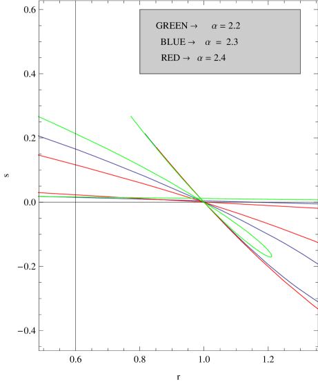
Figure 2: The variation of $s$ against $r$ for logamediate Scenario with $A=1$ and $\alpha=2.2,2.3,2.4$

From (2) we get the total energy density of the universe,

$$\rho_{tot}=3H^{2}=\frac{3A^{2}\alpha^{2}(\ln t)^{2\alpha-2}}{t^{2}}$$ (13)

II.2 Intermediate Scenario

Consider a particular form of Intermediate Scenario [25], where the scale factor $a(t)$ of the Friedmann universe is described as,

$$a(t)=\exp(Bt^{\beta})$$ (14)

where $B\beta>0$, $B>0$ and $0<\beta<1$. Here the expansion of Universe is faster than Power-Law form, where the scale factor is given as, $a(t)=t^{n}$, where $n>1$ is a constant. Also, the expansion of the Universe is slower for Standard de-Sitter Scenario where $\beta=1$. The Hubble parameter $H=\frac{\dot{a}}{a}$ becomes,

$$H=B\beta t^{\beta-1}$$ (15)

Hence from (15) we get,

$$\frac{\dot{H}}{H}=\frac{\beta-1}{t}$$ (16)

and

$$\frac{\ddot{H}}{H}=\frac{(\beta-1)(\beta-2)}{t^{2}}$$ (17)

Putting the value of $a(t)$ in the deceleration parameter $q=-\frac{a{\ddot{a}}}{{\dot{a}}^{2}}$ we get,

$$q=-1-\frac{\beta-1}{B\beta t^{\beta}}$$ (18)

where $a(t)$ is the scale factor. It has been seen that $q>-1$. Fig.3 represents the variation of $H$ against $q$ for different values of $\beta$.

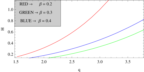
Figure 3: The variation of $H$ against $q$ for intermediate Scenario with $B=1$ and $\beta=0.2,0.3,0.4$

From (10), we get the expressions for statefinder parameters as

$$r=1+\frac{(\beta-1)(\beta-2)}{B^{2}\beta^{2}}t^{-2\beta}+\frac{\beta+1}{B\beta}t^{-\beta}$$ (19)

and

$$s=-\frac{\frac{(\beta-1)(\beta-2)}{B\beta t^{\beta}}+\beta+1}{3(\beta-1)+\frac{9B\beta t^{\beta}}{2}}$$ (20)

Fig.4 represents the variation of $s$ against $r$ for different values of $\beta$. We see that $r$ increases with increasing $s$. At the evolution of the universe, $r$ and $s$ are both increase and keep positive sign always.

From (2) we get the total energy density of the universe,

$$\rho_{tot}=3H^{2}=3B^{2}\beta^{2}t^{2\beta-2}$$ (21)

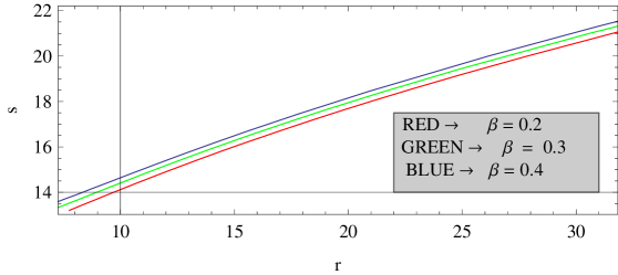
Figure 4: The variation of $s$ against $r$ for intermediate Scenario with $B=1$ and $\beta=0.2,0.3,0.4$

III Mixture of Generalized Chaplygin Gas with Tachyonic Field

The Lagrangian density for the tachyonic field is denoted as $\cal L$, defined as [15],

$${\cal{L}}=-V(\phi)\sqrt{1+g^{\mu\nu}~{}\partial{{}_{\mu}}\phi\partial{{}_{\nu}}\phi}$$ (22)

where $\phi$ is the tachyonic field and $V(\phi)$ is the tachyonic potential. The homogeneous tachyon condensate of string theory in a gravitational background is given by,

$$S=\int{\sqrt{-g}~{}d^{4}x\left[\frac{\cal R}{16\pi G}+{\cal L}\right]}$$ (23)

where $\cal R$ is the Ricci Scalar. The energy-momentum tensor for the tachyonic field is,

$$T_{\mu\nu}=-V(\phi)\sqrt{1+g^{\mu\nu}\partial_{\mu}\phi\partial_{\nu}\phi}~{}g^{\mu\nu}+V(\phi)\frac{\partial_{\mu}\phi\partial_{\nu}\phi}{\sqrt{1+g^{\mu\nu}\partial_{\mu}\phi\partial_{\nu}\phi}}$$ (24)

where the velocity $u_{\mu}$ is given by,

$$u_{\mu}=-\frac{\partial_{\mu}\phi}{\sqrt{-g^{\mu\nu}\partial_{\mu}\phi\partial_{\nu}\phi}}$$ (25)

with $u^{\nu}u_{\nu}=-1$.

So the energy density $\rho_{t}$ and the pressure $p_{t}$ of the tachyonic field $\phi$ become

$$\rho_{t}=\frac{V(\phi)}{\sqrt{1-{\dot{\phi}}^{2}}}~{}~{}~{}~{}~{}\text{and}~{}~{}~{}~{}~{}p_{t}=-V(\phi)\sqrt{1-{\dot{\phi}}^{2}}$$ (26)

Hence from (26) we get,

$$\phi=\int\sqrt{1+\frac{p_{t}}{\rho_{t}}}~{}dt$$ (27)

and

$$V(\phi)=\sqrt{-p_{t}\rho_{t}}$$ (28)

which represents pure Chaplygin gas if $V(\phi)$ is assumed as a constant (i.e. $p_{t}$ and $\rho_{t}$ are inversely proportional).

In the class of scalar potentials, Barrow [25] has assumed slow-roll inflation, $3H\dot{\phi}\approx-dV/d\phi$. Indeed, as field rolls down the potential towards larger values, the slow-roll approximation becomes increasingly more accurate. In the Hamilton-Jacobi formalism, the slow-roll-parameters are defined as [25],

$$\epsilon=2\left(\frac{H^{\prime}}{H}\right)^{2}=\frac{2{\dot{H}}^{2}}{H^{2}\dot{\phi}^{2}}$$ (29)

and

$$\eta=\frac{2H^{\prime\prime}}{H}=\frac{2}{H}\left(\frac{\ddot{H}}{\dot{\phi}^{2}}-\frac{\dot{H}\ddot{\phi}}{\dot{\phi}^{3}}\right)$$ (30)

where DOT indicates differentiation w.r.t. $t$ and DASH indicates differentiation w.r.t. $\phi$. Barrow [25] has shown that the slow-roll parameter $\epsilon$ diverges when the field approaches zero, has a minimum at the maximum of the potential, peaks at some value $\phi_{\epsilon}$, and finally asymptotes to zero for large values of the field. It has been shown that the peak occurs for $\epsilon>1$, so that at the moment when inflation begins with $\phi_{1}\equiv\phi(\epsilon=1)$.

For the accelerated expansion of the universe, we search a new type of matter i.e., dark energy which violates the strong energy condition. Pure Chaplygin Gas (PCG) is a particular type of dark energy, which obeys an equation of state, $p=-C/\rho$ [8-12], where $p$ and $\rho$ are the pressure and energy density of the PCG respectively where $C$ is a positive constant. The PCG was modified to generalized Chaplygin gas (MCG), which obeys an equation of state, $p=-C/\rho^{\gamma}$ where $0\leq\gamma\leq 1$. The GCG is modified to Modified Chaplygin Gas [13,14] obeying an equation of state $p=A\rho-C/\rho^{\gamma}$ with $0\leq\gamma\leq 1$, where $A,~{}C$ are positive constants. This equation of state shows radiation era at one extreme and a $\Lambda$CDM model at the other extreme.

Let us consider the universe is filled with the mixture of generalized Chaplygin Gas and tachyonic field. This generalized Chaplygin Gas is considered a perfect fluid which follows the adiabatic equation of state. The equation of Generalized Chaplygin Gas is given by,

$$p_{c}=-C/{\rho}_{c}^{\gamma}~{}~{},~{}~{}~{}0\leq\gamma\leq 1,C>0.$$ (31)

If the energy density of the fluid is a function of volume only, the temperature of the fluid remains zero at any pressure or volume, violating the third law of thermodynamics. The total energy density and pressure are respectively given by,

$$\rho_{tot}=\rho_{c}+\rho_{t}$$ (32)

$$p_{tot}=p_{c}+p_{t}$$ (33)

where $p_{c}$ and $\rho_{c}$ are the pressure and density of the generalized Chaplygin gas respectively and $p_{t}$ and $\rho_{t}$ are the pressure and density of the Tachyonic field respectively. Now we consider two possible states: (i) Without interaction and (ii) With interaction.

III.1 Without Interaction

The energy conservation equation is,

$$\dot{\rho}_{tot}+3\frac{\dot{a}}{a}(\rho_{tot}+p_{tot})=0$$ (34)

Suppose two fluids do not interact with each other. Then the above equation may be written as,

$$\dot{\rho}_{t}+3\frac{\dot{a}}{a}(\rho_{t}+p_{t})=0$$ (35)

and

$$\dot{\rho}_{c}+3\frac{\dot{a}}{a}(\rho_{c}+p_{c})=0$$ (36)

Now from equations (31) and (36), after eliminating $p_{c}$ we get $\rho_{c}$ in terms of the scale factor,

$$\rho_{c}=\left[C+\rho_{0}a^{-3(1+\gamma)}\right]^{\frac{1}{1+\gamma}}$$ (37)

where $\rho_{0}$ is the integrating constant.

Case I:

In case of Logamediate Scenario using (5), equation (37) reduces to,

$$\rho_{c}=[C+\rho_{0}x_{1}]^{\frac{1}{(1+\gamma)}}$$ (38)

where, $x_{1}=\exp(-3A(1+\gamma)(\ln t)^{\alpha})$. Hence from (13) and (38) the energy density of the tachyonic fluid becomes

$$\rho_{t}=\frac{3A^{2}\alpha^{2}(\ln t)^{2\alpha-2}}{t^{2}}-[C+\rho_{0}x_{1}]^{\frac{1}{(1+\gamma)}}$$ (39)

Hence from (35) and (39) the pressure of the tachyonic fluid becomes,

$$p_{t}=-\frac{3A^{2}\alpha^{2}(\ln t)^{2\alpha-2}}{t^{2}}+\frac{2A\alpha(\ln t-\alpha+1)(\ln t)^{\alpha-2}}{t^{2}}+C[C+\rho_{0}x_{1}]^{\frac{-\gamma}{(1+\gamma)}}$$ (40)

Solving the equations (27), (28), (39) and (40), the tachyonic field and the tachyonic potential are obtained as,

$$\phi=\int\sqrt{\frac{\frac{2A\alpha(-\ln t+\alpha-1)(\ln t)^{\alpha-2}}{t^{2}}+\rho_{0}x_{1}[C+\rho_{0}x_{1}]^{\frac{-\gamma}{\gamma+1}}}{[C+\rho_{0}x_{1}]^{\frac{1}{\gamma+1}}-\frac{3A^{2}\alpha^{2}(\ln t)^{2\alpha-2}}{t^{2}}}}~{}dt$$ (41)

and

$$V(\phi)=\sqrt{\frac{3A^{2}\alpha^{2}(\ln t)^{2\alpha-2}}{t^{2}}-[C+\rho_{0}x_{1}]^{\frac{1}{(1+\gamma)}}}~{}~{}\times~{}~{}~{}~{}~{}~{}~{}~{}~{}~{}~{}~{}~{}~{}~{}~{}~{}~{}~{}~{}~{}~{}~{}~{}~{}~{}$$

$$\sqrt{\frac{3A^{2}\alpha^{2}(\ln t)^{2\alpha-2}}{t^{2}}-\frac{2A\alpha(\ln t-\alpha+1)(\ln t)^{\alpha-2}}{t^{2}}-C[C+\rho_{0}x_{1}]^{\frac{-\gamma}{(1+\gamma)}}}$$ (42)

Fig.5  represents the variation of $V$ against $\phi$ for different values of $\alpha$. In this case, the potential always decreases with the tachyonic field $\phi$.

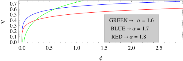
Figure 5: The variation of $V$ against $\phi$ from equations (41) and (42) for $A=C=1,\rho_{0}=5,\gamma=.5$ and $\alpha=1.6,1.7,1.8$

From (7), (8), (29), (30) and (41) we get the slow-roll parameters,

$$\epsilon=2\left(\frac{\alpha-1-\ln t}{t\ln t}\right)^{2}\times\frac{[C+\rho_{0}x_{1}]^{\frac{1}{\gamma+1}}-\frac{3A^{2}\alpha^{2}(\ln t)^{2\alpha-2}}{t^{2}}}{\frac{2A\alpha(-\ln t+\alpha-1)(\ln t)^{\alpha-2}}{t^{2}}+\rho_{0}x_{1}[C+\rho_{0}x_{1}]^{\frac{-\gamma}{\gamma+1}}}$$ (43)

and

$$\eta=2\times\frac{[C+\rho_{0}x_{1}]^{\frac{1}{\gamma+1}}-\frac{3A^{2}\alpha^{2}(\ln t)^{2\alpha-2}}{t^{2}}}{\frac{2A\alpha(-\ln t+\alpha-1)(\ln t)^{\alpha-2}}{t^{2}}+\rho_{0}x_{1}[C+\rho_{0}x_{1}]^{\frac{-\gamma}{\gamma+1}}}\times\left(\frac{2(\ln t)^{2}-3(\alpha-1)\ln t+(\alpha-1)(\alpha-2)}{t^{2}(\ln t)^{2}}\right)-$$

$$\left(\frac{\alpha-1-\ln t}{t\ln t}\right)\left(\frac{[C+\rho_{0}x_{1}]^{\frac{1}{\gamma+1}}-\frac{3A^{2}\alpha^{2}(\ln t)^{2\alpha-2}}{t^{2}}}{\frac{2A\alpha(-\ln t+\alpha-1)(\ln t)^{\alpha-2}}{t^{2}}+\rho_{0}x_{1}[C+\rho_{0}x_{1}]^{\frac{-\gamma}{\gamma+1}}}\right)^{2}\frac{\partial}{\partial{t}}\left[\frac{\frac{2A\alpha(-\ln t+\alpha-1)(\ln t)^{\alpha-2}}{t^{2}}+\rho_{0}x_{1}[C+\rho_{0}x_{1}]^{\frac{-\gamma}{\gamma+1}}}{[C+\rho_{0}x_{1}]^{\frac{1}{\gamma+1}}-\frac{3A^{2}\alpha^{2}(\ln t)^{2\alpha-2}}{t^{2}}}\right]$$ (44)

From the above equations, we see that $\eta$ can not be expressed explicitly in terms of $\epsilon$. So we draw the graph of $\eta$ against $\epsilon$ in Fig.6 for different values of $\alpha$.

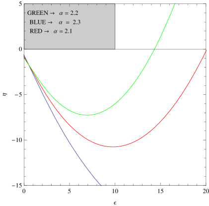
Figure 6: The variation of $\eta$ against $\epsilon$ from equations (43) and (44) for $A=C=1,\rho_{0}=5,\gamma=.5$ and $\alpha=2.1,2.2,2.3$

Case II:

In case of Intermediate Scenario, using (14), equation (37) reduces to,

$$\rho_{c}=[C+\rho_{0}x_{2}]^{\frac{1}{(1+\gamma)}}$$ (45)

where, $x_{2}=\exp(-3B(1+\gamma)t^{\beta})$.

Hence from (21), (33), (35) and (45) we get the energy density and the pressure of the tachyonic fluid is,

$$\rho_{t}=3B^{2}\beta^{2}t^{2\beta-2}-[C+\rho_{0}x_{2}]^{\frac{1}{(1+\gamma)}}$$ (46)

and

$$p_{t}=-3B^{2}\beta^{2}t^{2\beta-2}-2B\beta(\beta-1)t^{\beta-2}+C[C+\rho_{0}x_{2}]^{\frac{-\gamma}{(1+\gamma)}}$$ (47)

Solving the equations (27), (28), (46) and (47), the tachyonic field and the tachyonic potential are obtained as,

$$\phi=\int\sqrt{\frac{2B\beta(\beta-1)t^{\beta-2}-C[C+\rho_{0}x_{2}]^{\frac{-\gamma}{(1+\gamma)}}}{[C+\rho_{0}x_{2}]^{\frac{1}{(1+\gamma)}}-3B^{2}\beta^{2}t^{2\beta-2}}}dt$$ (48)

and

$$V(\phi)=\sqrt{3B^{2}\beta^{2}t^{2\beta-2}-[C+\rho_{0}x_{2}]^{\frac{1}{(1+\gamma)}}}\times\sqrt{3B^{2}\beta^{2}t^{2\beta-2}+2B\beta(\beta-1)t^{\beta-2}-C[C+\rho_{0}x_{2}]^{\frac{-\gamma}{(1+\gamma)}}}$$ (49)

Fig.7  represents the variation of $V$ against $\phi$ for different values of $\beta$. Here the potential $V$ is sharply decreasing with the tachyonic field $\phi$.

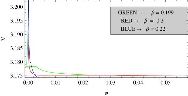
Figure 7: The variation of $V$ against $\phi$ from (48) and (49) for $C=2,\rho_{0}=5,\gamma=.5,B=1$ and $\beta=0.199,0.2,0.22$

From (16), (17), (29), (30) and (48) we get the slow-roll parameter,

$$\epsilon=2\left(\frac{\beta-1}{t}\right)^{2}\times\frac{[C+\rho_{0}x_{2}]^{\frac{1}{(1+\gamma)}}-3B^{2}\beta^{2}t^{2\beta-2}}{2B\beta(\beta-1)t^{\beta-2}-C[C+\rho_{0}x_{2}]^{\frac{-\gamma}{(1+\gamma)}}}$$ (50)

and

$$\eta=\frac{2(\beta-1)(\beta-2)}{t^{2}}\times\frac{[C+\rho_{0}x_{2}]^{\frac{1}{(1+\gamma)}}-3B^{2}\beta^{2}t^{2\beta-2}}{2B\beta(\beta-1)t^{\beta-2}-C[C+\rho_{0}x_{2}]^{\frac{-\gamma}{(1+\gamma)}}}-$$

$$\left(\frac{\beta-1}{t}\right)\left(\frac{[C+\rho_{0}x_{2}]^{\frac{1}{(1+\gamma)}}-3B^{2}\beta^{2}t^{2\beta-2}}{2B\beta(\beta-1)t^{\beta-2}-C[C+\rho_{0}x_{2}]^{\frac{-\gamma}{(1+\gamma)}}}\right)^{2}\frac{\partial}{\partial{t}}\left[\frac{2B\beta(\beta-1)t^{\beta-2}-C[C+\rho_{0}x_{2}]^{\frac{-\gamma}{(1+\gamma)}}}{[C+\rho_{0}x_{2}]^{\frac{1}{(1+\gamma)}}-3B^{2}\beta^{2}t^{2\beta-2}}\right]$$ (51)

Fig.8  represents the variation of $\eta$ against $\epsilon$ for different values of $\beta$. From this figure, it has been seen that $\eta$ is sharply decreasing with increasing $\epsilon$.

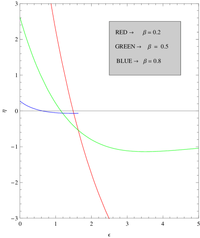
Figure 8: The variation of $\eta$ against $\epsilon$ from (50) and (51) for $C=2,\gamma=.5,\rho_{0}=5,B=1$ and $\beta=0.2,0.5,0.8$

III.2 With Interaction

Now we consider an interaction between the tachyonic fluid and GCG by introducing an interaction term as a product of the Hubble parameter and the energy density of the Chaplygin gas. Thus there is an energy flow between the two fluids.

Now the equations of motion corresponding to the tachyonic field and GCG are respectively,

$$\dot{\rho}_{t}+3\frac{\dot{a}}{a}(\rho_{t}+p_{t})=-3H\delta\rho_{c}$$ (52)

and

$$\dot{\rho}_{c}+3\frac{\dot{a}}{a}(\rho_{c}+p_{c})=3H\delta\rho_{c}$$ (53)

where $\delta$ is a coupling constant.

Solving equation (53) with the help of equations (14) and (31) we get,

$$\rho_{c}=\left[\frac{C}{1-\delta}+\rho_{0}a^{-3(1+\gamma)(1-\delta)}\right]^{\frac{1}{(1+\gamma)}}$$ (54)

Case I:

In case of Logamediate Scenario, we get the solutions:

$$\rho_{c}=\left[\frac{C}{1-\delta}+\rho_{0}x_{3}\right]^{\frac{1}{(1+\gamma)}}$$ (55)

$$\rho_{t}=\frac{3A^{2}\alpha^{2}(\ln t)^{2\alpha-2}}{t^{2}}-\left[\frac{C}{1-\delta}+\rho_{0}x_{3}\right]^{\frac{1}{(1+\gamma)}}$$ (56)

where $x_{3}=\exp(-3A(1-\delta)(1+\gamma)(\ln t)^{\alpha})$. Hence,

$$p_{t}=-\frac{3A^{2}\alpha^{2}(\ln t)^{2\alpha-2}}{t^{2}}+\frac{2A\alpha(\ln t-\alpha+1)(\ln t)^{\alpha-2}}{t^{2}}+C\left[\frac{C}{1-\delta}+\rho_{0}x_{3}\right]^{\frac{-\gamma}{(1+\gamma)}}$$ (57)

Solving the equations, the tachyonic field is obtained as,

$$\phi=\int\sqrt{\frac{\frac{2A\alpha(\ln t-\alpha+1)(\ln t)^{\alpha-2}}{t^{2}}-\left(\frac{C\delta}{1-\delta}+\rho_{0}x_{3}\right)\left(\frac{C}{1-\delta}+\rho_{0}x_{3}\right)^{\frac{-\gamma}{1+\gamma}}}{\frac{3A^{2}\alpha^{2}(\ln t)^{2\alpha-2}}{t^{2}}-\left[\frac{C}{1-\delta}+\rho_{0}x_{3}\right]^{\frac{1}{(1+\gamma)}}}}~{}dt$$ (58)

Also the potential will be of the form,

$$V(\phi)=\sqrt{\frac{3A^{2}\alpha^{2}(\ln t)^{2\alpha-2}}{t^{2}}-\left[\frac{C}{1-\delta}+\rho_{0}x_{3}\right]^{\frac{1}{(1+\gamma)}}}~{}~{}\times$$

$$\sqrt{\frac{3A^{2}\alpha^{2}(\ln t)^{2\alpha-2}}{t^{2}}-\frac{2A\alpha(\ln t-\alpha+1)(\ln t)^{\alpha-2}}{t^{2}}-C\left[\frac{C}{1-\delta}+\rho_{0}x_{3}\right]^{\frac{-\gamma}{(1+\gamma)}}}$$ (59)

In this case the potential starting from a large value and finally tends to small value (Fig.9).

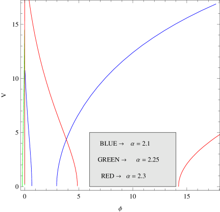
Figure 9: The variation of $V$ against $\phi$ from (58) and (59) for $A=C=1,\rho_{0}=5,\gamma=.5,\delta=.2$ and $\alpha=2.1,2.25,2.3$

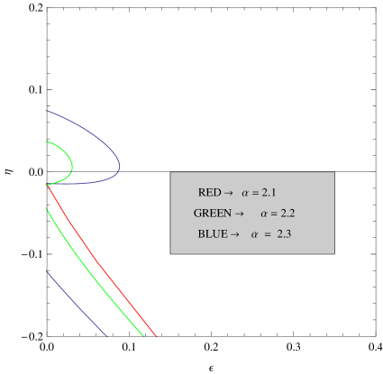
Figure 10: The variation of $\eta$ against $\epsilon$ from (60) and (61) for $A=C=1,\rho_{0}=5,\delta=.2,\gamma=.5$ and $\alpha=2.1,2.2,2.3$

The slow-roll parameters are obtained as

$$\epsilon=2\left(\frac{\alpha-1-\ln t}{t\ln t}\right)^{2}\times\frac{\frac{3A^{2}\alpha^{2}(\ln t)^{2\alpha-2}}{t^{2}}-\left[\frac{C}{1-\delta}+\rho_{0}x_{3}\right]^{\frac{1}{(1+\gamma)}}}{\frac{2A\alpha(\ln t-\alpha+1)(\ln t)^{\alpha-2}}{t^{2}}-\left(\frac{C\delta}{1-\delta}+\rho_{0}x_{3}\right)\left(\frac{C}{1-\delta}+\rho_{0}x_{3}\right)^{\frac{-\gamma}{1+\gamma}}}$$ (60)

and

$$\eta=2\times\frac{\frac{3A^{2}\alpha^{2}(\ln t)^{2\alpha-2}}{t^{2}}-\left[\frac{C}{1-\delta}+\rho_{0}x_{3}\right]^{\frac{1}{(1+\gamma)}}}{\frac{2A\alpha(\ln t-\alpha+1)(\ln t)^{\alpha-2}}{t^{2}}-\left(\frac{C\delta}{1-\delta}+\rho_{0}x_{3}\right)\left(\frac{C}{1-\delta}+\rho_{0}x_{3}\right)^{\frac{-\gamma}{1+\gamma}}}\times\frac{2(\ln t)^{2}-3(\alpha-1)\ln t+(\alpha-1)(\alpha-2)}{t^{2}(\ln t)^{2}}-$$

$$\left(\frac{\alpha-1-\ln t}{t\ln t}\right)\times\frac{\frac{3A^{2}\alpha^{2}(\ln t)^{2\alpha-2}}{t^{2}}-\left[\frac{C}{1-\delta}+\rho_{0}x_{3}\right]^{\frac{1}{(1+\gamma)}}}{\frac{2A\alpha(\ln t-\alpha+1)(\ln t)^{\alpha-2}}{t^{2}}-\left(\frac{C\delta}{1-\delta}+\rho_{0}x_{3}\right)\left(\frac{C}{1-\delta}+\rho_{0}x_{3}\right)^{\frac{-\gamma}{1+\gamma}}}\times$$

$$\frac{\partial}{\partial{t}}\left[\frac{\frac{2A\alpha(\ln t-\alpha+1)(\ln t)^{\alpha-2}}{t^{2}}-\left(\frac{C\delta}{1-\delta}+\rho_{0}x_{3}\right)\left(\frac{C}{1-\delta}+\rho_{0}x_{3}\right)^{\frac{-\gamma}{1+\gamma}}}{\frac{3A^{2}\alpha^{2}(\ln t)^{2\alpha-2}}{t^{2}}-\left[\frac{C}{1-\delta}+\rho_{0}x_{3}\right]^{\frac{1}{(1+\gamma)}}}\right]$$ (61)

From above expressions of $\epsilon$ and $\eta$, we see that $\eta$ can not be expressed in terms of $\epsilon$. So we have drawn the graph of $\eta$ against $\epsilon$ in Fig.10.

Case II:

In case of Intermediate Scenario, using (1), equation (36) reduces to,

$$\rho_{c}=\left[\frac{C}{1-\delta}+\rho_{0}x_{4}\right]^{\frac{1}{(1+\gamma)}}$$

where $x_{4}=\exp(-3B(1-\delta)(1+\gamma)t^{\beta})$. Hence the energy density of the tachyonic fluid is,

$$\rho_{t}=3B^{2}\beta^{2}t^{2\beta-2}-\left[\frac{C}{1-\delta}+\rho_{0}x_{4}\right]^{\frac{1}{(1+\gamma)}}$$ (62)

Hence the pressure of the tachyonic fluid is,

$$p_{t}=-3B^{2}\beta^{2}t^{2\beta-2}-2B\beta(\beta-1)t^{\beta-2}-\rho_{0}(1-\delta)(1+\gamma)x_{4}\left[\frac{C}{1-\delta}+\rho_{0}x_{4}\right]^{\frac{-\gamma}{(1+\gamma)}}$$ (63)

Solving the equations the tachyonic field and the tachyonic potential are obtained as,

$$\phi=\int\sqrt{\frac{2B\beta(\beta-1)t^{\beta-2}-\left[\frac{C}{1-\delta}+\rho_{0}x_{4}\right]^{\frac{1}{(1+\gamma)}}+\rho_{0}(1-\delta)(1+\gamma)x_{4}\left[\frac{C}{1-\delta}+\rho_{0}x_{4}\right]^{\frac{-\gamma}{(1+\gamma)}}}{\left[\frac{C}{1-\delta}+\rho_{0}x_{4}\right]^{\frac{1}{(1+\gamma)}}-3B^{2}\beta^{2}t^{2\beta-2}}}~{}dt$$ (64)

and

$$V(\phi)=\sqrt{3B^{2}\beta^{2}t^{2\beta-2}-\left[\frac{C}{1-\delta}+\rho_{0}x_{4}\right]^{\frac{1}{(1+\gamma)}}}~{}~{}\times$$

$$\sqrt{3B^{2}\beta^{2}t^{2\beta-2}+2B\beta(\beta-1)t^{\beta-2}+\rho_{0}(1-\delta)(1+\gamma)x_{4}\left[\frac{C}{1-\delta}+\rho_{0}x_{4}\right]^{\frac{-\gamma}{(1+\gamma)}}}$$ (65)

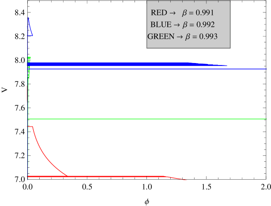
Figure 11: The variation of $V$ against $\phi$ from (64) and (65) for $B=1,C=2,\rho_{0}=5,\gamma=\delta=.5$ and $\beta=0.991,0.992,0.993$

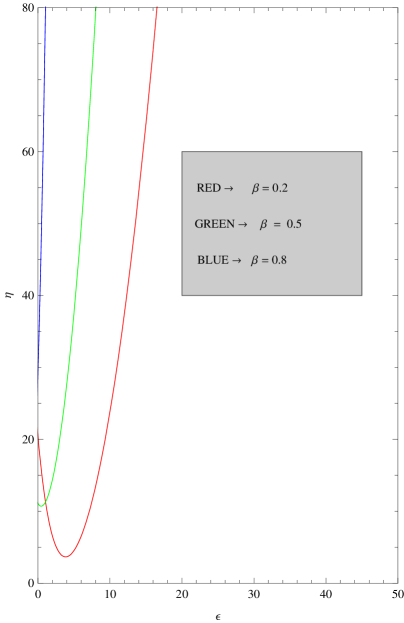
Figure 12: The variation of $\eta$ against $\epsilon$ from (66) and (67) for $B=1,C=2,\rho_{0}=5,\gamma=\delta=.5$ and $\beta=0.2,0.5,0.8$

Fig.11  represents the variation of $V$ against $\phi$ for different values of $\beta$. Here the potential $V$ decreases with the tachyonic field $\phi$.

The slow-roll parameters will be,

$$\epsilon=2\left(\frac{\beta-1}{t}\right)^{2}\times\frac{\left[\frac{C}{1-\delta}+\rho_{0}x_{4}\right]^{\frac{1}{(1+\gamma)}}-3B^{2}\beta^{2}t^{2\beta-2}}{2B\beta(\beta-1)t^{\beta-2}-\left[\frac{C}{1-\delta}+\rho_{0}x_{4}\right]^{\frac{1}{(1+\gamma)}}+\rho_{0}(1-\delta)(1+\gamma)x_{4}\left[\frac{C}{1-\delta}+\rho_{0}x_{4}\right]^{\frac{-\gamma}{(1+\gamma)}}}$$ (66)

and

$$\eta=\frac{2(\beta-1)(\beta-2)}{t^{2}}\times\frac{\left[\frac{C}{1-\delta}+\rho_{0}x_{4}\right]^{\frac{1}{(1+\gamma)}}-3B^{2}\beta^{2}t^{2\beta-2}}{2B\beta(\beta-1)t^{\beta-2}-\left[\frac{C}{1-\delta}+\rho_{0}x_{4}\right]^{\frac{1}{(1+\gamma)}}+\rho_{0}(1-\delta)(1+\gamma)x_{4}\left[\frac{C}{1-\delta}+\rho_{0}x_{4}\right]^{\frac{-\gamma}{(1+\gamma)}}}$$

$$-\left(\frac{\beta-1}{t}\right)\times\left(\frac{\left[\frac{C}{1-\delta}+\rho_{0}x_{4}\right]^{\frac{1}{(1+\gamma)}}-3B^{2}\beta^{2}t^{2\beta-2}}{2B\beta(\beta-1)t^{\beta-2}-\left[\frac{C}{1-\delta}+\rho_{0}x_{4}\right]^{\frac{1}{(1+\gamma)}}+\rho_{0}(1-\delta)(1+\gamma)x_{4}\left[\frac{C}{1-\delta}+\rho_{0}x_{4}\right]^{\frac{-\gamma}{(1+\gamma)}}}\right)^{2}\times$$

$$\frac{\partial}{\partial{t}}\left[\frac{2B\beta(\beta-1)t^{\beta-2}-\left[\frac{C}{1-\delta}+\rho_{0}x_{4}\right]^{\frac{1}{(1+\gamma)}}+\rho_{0}(1-\delta)(1+\gamma)x_{4}\left[\frac{C}{1-\delta}+\rho_{0}x_{4}\right]^{\frac{-\gamma}{(1+\gamma)}}}{\left[\frac{C}{1-\delta}+\rho_{0}x_{4}\right]^{\frac{1}{(1+\gamma)}}-3B^{2}\beta^{2}t^{2\beta-2}}\right]$$ (67)

From fig.12, it has been seen that $\eta$ first decreases then increases with $\epsilon$.

IV Mixture of Barotropic Fluid with Tachyonic Field

A barotropic fluid is defined as that state of a fluid for which is a function of only the pressure. The condition of barotropy of a fluid represents another rather idealized state. However, in this case the situation is closer to reality since compressibility is allowed for. The term “barotropic” infers “turning with (or in the same manner as) the isobars”, referring to the isopycnals. The name is a lucid one since it is obvious that if depends only on $p$ then the isopycnal surfaces must always be parallel to the isobaric surfaces, hence any change in inclination of the latter brings about an identical change in orientation of the isopycnal surfaces. The spacing of the isobaric surfaces with respect to under quasistatic conditions depends only on $p$ for a barotropic fluid. Furthermore, since is increased with increasing pressure for a compressible fluid it is apparent that the spacing of isobaric surfaces (for equal increments of $p$) relative to will decrease with increasing $p$.

A fluid under conditions of perfect hydrostatic balance would assume a barotropic state for which the pressure gradient can be represented as a function of $p$ alone. However, this is a very special case of barotropy where the isobaric surfaces are level. Now we consider a two fluid model consisting of tachyonic field and barotropic fluid. The EOS of the barotropic fluid is given by,

$$p_{b}=\omega_{b}\rho_{b}$$ (68)

where $p_{b}$ and $\rho_{b}$ are the pressure and energy density of the barotropic fluid. Hence the total energy density and pressure are respectively given by,

$$\rho_{tot}=\rho_{b}+\rho_{t}$$ (69)

and

$$p_{tot}=p_{b}+p_{t}$$ (70)

IV.1 Without Interaction

First we consider that the two fluids do not interact with each other so that they are conserved separately. Therefore, the conservation equation (34) reduces to,

$$\dot{\rho}_{t}+3\frac{\dot{a}}{a}(\rho_{t}+p_{t})=0$$ (71)

and

$$\dot{\rho}_{b}+3\frac{\dot{a}}{a}(\rho_{b}+p_{b})=0$$ (72)

Equation (72) together with equation (68) give,

$$\rho_{b}=\rho_{0}~{}a^{-3(1+\omega_{b})}$$ (73)

Case I:

In case of Logamediate Scenario, using (5), equation (73) reduces to,

$$\rho_{b}=\rho_{0}\exp(-3A(1+\omega_{b})(\ln t)^{\alpha})$$ (74)

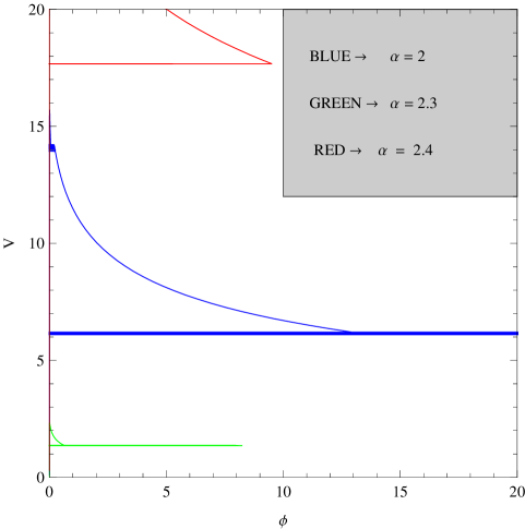
Figure 13: The variation of $V$ against $\phi$ from (77) and (78) for $A=1,\rho_{0}=5,\omega=.2$ and $\alpha=2,2.3,2.4$

Hence the energy density of the tachyonic fluid is,

$$\rho_{t}=\frac{3A^{2}\alpha^{2}(\ln t)^{2\alpha-2}}{t^{2}}-\rho_{0}x_{5}$$ (75)

where, $x_{5}=\exp(-3A(1+\omega_{b})(\ln t)^{\alpha})$. Hence the pressure of the tachyonic fluid is,

$$p_{t}=-\frac{3A^{2}\alpha^{2}(\ln t)^{2\alpha-2}}{t^{2}}+\frac{2A\alpha(\ln t-\alpha+1)(\ln t)^{\alpha-2}}{t^{2}}-\rho_{0}\omega_{b}x_{5}$$ (76)

Solving the equations the tachyonic field and the tachyonic potential are obtained as,

$$\phi=\int\sqrt{\frac{\frac{2A\alpha(\ln t-\alpha+1)(\ln t)^{\alpha-2}}{t^{2}}-\rho_{0}(1+\omega_{b})x_{5}}{\frac{3A^{2}\alpha^{2}(\ln t)^{2\alpha-2}}{t^{2}}-\rho_{0}x_{5}}}dt$$ (77)

and

$$V(\phi)=\sqrt{\frac{3A^{2}\alpha^{2}(\ln t)^{2\alpha-2}}{t^{2}}-\rho_{0}x_{5}}\times\sqrt{\frac{3A^{2}\alpha^{2}(\ln t)^{2\alpha-2}}{t^{2}}-\frac{2A\alpha(\ln t-\alpha+1)(\ln t)^{\alpha-2}}{t^{2}}+\rho_{0}\omega_{b}x_{5}}$$ (78)

From above equations, it has been seen that $V$ can not be expressed in terms of $\phi$ explicitly. Fig. 13 shows the variation of $V$ in terms of $\phi$.

The slow-roll parameters are obtained as,

$$\epsilon=2\left(\frac{\alpha-1-\ln t}{t\ln t}\right)^{2}\times\frac{\frac{3A^{2}\alpha^{2}(\ln t)^{2\alpha-2}}{t^{2}}-\rho_{0}x_{5}}{\frac{2A\alpha(\ln t-\alpha+1)(\ln t)^{\alpha-2}}{t^{2}}-\rho_{0}(1+\omega_{b})x_{5}}$$ (79)

and

$$\eta=2\times\frac{\frac{3A^{2}\alpha^{2}(\ln t)^{2\alpha-2}}{t^{2}}-\rho_{0}x_{5}}{\frac{2A\alpha(\ln t-\alpha+1)(\ln t)^{\alpha-2}}{t^{2}}-\rho_{0}(1+\omega_{b})x_{5}}\times\left(\frac{2(\ln t)^{2}-3(\alpha-1)\ln t+(\alpha-1)(\alpha-2)}{t^{2}(\ln t)^{2}}\right)$$

$$-\left(\frac{\alpha-1-\ln t}{t\ln t}\right)\times\left(\frac{\frac{3A^{2}\alpha^{2}(\ln t)^{2\alpha-2}}{t^{2}}-x_{5}}{\frac{2A\alpha(\ln t-\alpha+1)(\ln t)^{\alpha-2}}{t^{2}}-\rho_{0}(1+\omega_{b})x_{5}}\right)^{2}\times\frac{\partial}{\partial{t}}\left[\frac{\frac{2A\alpha(\ln t-\alpha+1)(\ln t)^{\alpha-2}}{t^{2}}-\rho_{0}(1+\omega_{b})x_{5}}{\frac{3A^{2}\alpha^{2}(\ln t)^{2\alpha-2}}{t^{2}}-\rho_{0}x_{5}}\right]$$ (80)

From complicated forms of $\eta$ and $\epsilon$, it has been seen that $\eta$ can not be expressed in terms of $\epsilon$ explicitly. So we have shown the graph of $\eta$ with $\epsilon$ in fig. 14.

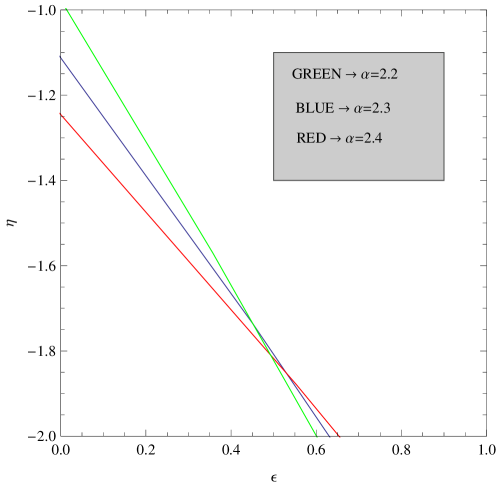
Figure 14: The variation of $\eta$ against $\epsilon$ from (79) and (80) for $A=1,\omega_{b}=.2,\rho_{0}=5$ and $\alpha=2.2,2.3,2.4$

Case II:

In case of Intermediate Scenario, using (14), equation (73) reduces to,

$$\rho_{b}=\rho_{0}\exp(-3B(1+\omega_{b})t^{\beta})$$ (81)

Hence the energy density of the tachyonic fluid is,

$$\rho_{t}=3B^{2}\beta^{2}t^{2\beta-2}-\rho_{0}x_{6}$$ (82)

where, $x_{6}=\exp(-3B(1+\omega_{b})t^{\beta})$. Hence the pressure of the tachyonic fluid is,

$$p_{t}=-3B^{2}\beta^{2}t^{2\beta-2}-2B\beta(\beta-1)t^{\beta-2}-\rho_{0}\omega_{b}x_{6}$$ (83)

Solving the equations the tachyonic field and the tachyonic potential are obtained as,

$$\phi=\int\sqrt{\frac{2B\beta(\beta-1)t^{\beta-2}+\rho_{0}(1+\omega_{b})x_{6}}{\rho_{0}x_{6}-3B^{2}\beta^{2}t^{2\beta-2}}}dt$$ (84)

and

$$V(\phi)=\sqrt{3B^{2}\beta^{2}t^{2\beta-2}-\rho_{0}x_{6}}\times\sqrt{3B^{2}\beta^{2}t^{2\beta-2}+2B\beta(\beta-1)t^{\beta-2}+\rho_{0}\omega_{b}x_{6}}$$ (85)

Like the mixture of tachyonic fluid with barotropic fluid in this case also the potential $V$ starting from a low value increases largely and then decreases to $0$ with time as shown in figure 15.

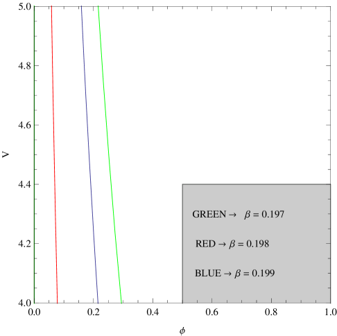
Figure 15: The variation of $V$ against $\phi$ from (84) and (85) for $B=1,\omega_{b}=\frac{1}{3},\rho_{0}=5$ and $\beta=0.197,0.198,0.199$

The slow-roll parameters will be,

$$\epsilon=2\left(\frac{\beta-1}{t}\right)^{2}\times\frac{\rho_{0}x_{6}-3B^{2}\beta^{2}t^{2\beta-2}}{2B\beta(\beta-1)t^{\beta-2}+\rho_{0}(1+\omega_{b})x_{6}}$$ (86)

and

$$\eta=\frac{2(\beta-1)(\beta-2)}{t^{2}}\times\frac{\rho_{0}x_{6}-3B^{2}\beta^{2}t^{2\beta-2}}{2B\beta(\beta-1)t^{\beta-2}+\rho_{0}(1+\omega_{b})x_{6}}-\left(\frac{\beta-1}{t}\right)\times$$

$$\left(\frac{\rho_{0}x_{6}-3B^{2}\beta^{2}t^{2\beta-2}}{2B\beta(\beta-1)t^{\beta-2}+\rho_{0}(1+\omega_{b})x_{6}}\right)^{2}\times\frac{\partial}{\partial{t}}\left[\frac{2B\beta(\beta-1)t^{\beta-2}+\rho_{0}(1+\omega_{b})x_{6}}{\rho_{0}x_{6}-3B^{2}\beta^{2}t^{2\beta-2}}\right]$$ (87)

From Fig.16 it has been seen that $\eta$ always decreases with $\epsilon$.

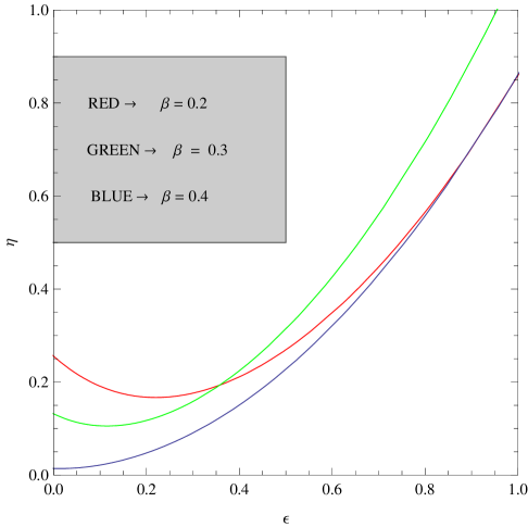
Figure 16: The variation of $\eta$ against $\epsilon$ from (86) and (87) for $B=1,\omega_{b}=1/3,\rho_{0}=5$ and $\beta=0.2,0.3,0.4$

IV.2 With Interaction

Now we consider an interaction between the tachyonic field and the barotropic fluid by introducing a phenomenological coupling function which is a product of the Hubble parameter and the energy density of the barotropic fluid. Thus there is an energy flow between the two fluids.

Now the equations of motion corresponding to the tachyonic field and the barotropic fluid are respectively,

$$\dot{\rho}_{t}+3\frac{\dot{a}}{a}(\rho_{t}+p_{t})=-3H\delta\rho_{b}$$ (88)

and

$$\dot{\rho}_{b}+3\frac{\dot{a}}{a}(\rho_{b}+p_{b})=3H\delta\rho_{b}$$ (89)

where $\delta$ is a coupling constant.

Solving equation (89) with the help of equation (68), we get,

$$\rho_{b}=\rho_{0}~{}a^{-3(1+\omega_{b}-\delta)}$$ (90)

Case I:

In case of Logamediate Scenario, we obtain

$$\rho_{t}=\frac{3A^{2}\alpha^{2}(\ln t)^{2\alpha-2}}{t^{2}}-\rho_{0}x_{7}$$ (91)

where, $x_{7}=\exp(-3A(1+\omega_{b}-\delta)(\ln t)^{\alpha})$. Hence,

$$p_{t}=-\frac{3A^{2}\alpha^{2}(\ln t)^{2\alpha-2}}{t^{2}}+\frac{2A\alpha(\ln t-\alpha+1)(\ln t)^{\alpha-2}}{t^{2}}-\rho_{0}\omega_{b}x_{7}$$ (92)

Solving the equations the tachyonic field is obtained as,

$$\phi=\int\sqrt{\frac{\frac{2A\alpha(\ln t-\alpha+1)(\ln t)^{\alpha-2}}{t^{2}}-\rho_{0}(1+\omega_{b})x_{7}}{\frac{3A^{2}\alpha^{2}(\ln t)^{2\alpha-2}}{t^{2}}-\rho_{0}x_{7}}}dt$$ (93)

Also the potential will be of the form,

$$V(\phi)=\sqrt{\frac{3A^{2}\alpha^{2}(\ln t)^{2\alpha-2}}{t^{2}}-\rho_{0}x_{7}}\times\sqrt{\frac{3A^{2}\alpha^{2}(\ln t)^{2\alpha-2}}{t^{2}}-\frac{2A\alpha(\ln t-\alpha+1)(\ln t)^{\alpha-2}}{t^{2}}+\rho_{0}\omega_{b}x_{7}}$$ (94)

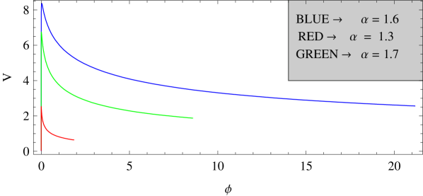
Figure 17: The variation of $V$ against $\phi$ from (93) and (94) for $A=1,\omega_{b}=.2,\rho_{0}=5,\delta=.5$ and $\alpha=1.3,1.6,1.7$

The slow-roll parameters are obtained as

$$\epsilon=2\left(\frac{\alpha-1-\ln t}{t\ln t}\right)^{2}\times\frac{\frac{3A^{2}\alpha^{2}(\ln t)^{2\alpha-2}}{t^{2}}-\rho_{0}x_{7}}{\frac{2A\alpha(\ln t-\alpha+1)(\ln t)^{\alpha-2}}{t^{2}}-\rho_{0}(1+\omega_{b})x_{7}}$$ (95)

and

$$\eta=2\times\frac{\frac{3A^{2}\alpha^{2}(\ln t)^{2\alpha-2}}{t^{2}}-\rho_{0}x_{7}}{\frac{2A\alpha(\ln t-\alpha+1)(\ln t)^{\alpha-2}}{t^{2}}-\rho_{0}(1+\omega_{b})x_{7}}\times\frac{2(\ln t)^{2}-3(\alpha-1)\ln t+(\alpha-1)(\alpha-2)}{t^{2}(\ln t)^{2}}$$

$$-\left(\frac{\alpha-1-\ln t}{t\ln t}\right)\times\left(\frac{\frac{3A^{2}\alpha^{2}(\ln t)^{2\alpha-2}}{t^{2}}-\rho_{0}x_{7}}{\frac{2A\alpha(\ln t-\alpha+1)(\ln t)^{\alpha-2}}{t^{2}}-\rho_{0}(1+\omega_{b})x_{7}}\right)^{2}\times\frac{\partial}{\partial{t}}\left[\frac{\frac{2A\alpha(\ln t-\alpha+1)(\ln t)^{\alpha-2}}{t^{2}}-\rho_{0}(1+\omega_{b})x_{7}}{\frac{3A^{2}\alpha^{2}(\ln t)^{2\alpha-2}}{t^{2}}-\rho_{0}x_{7}}\right]$$ (96)

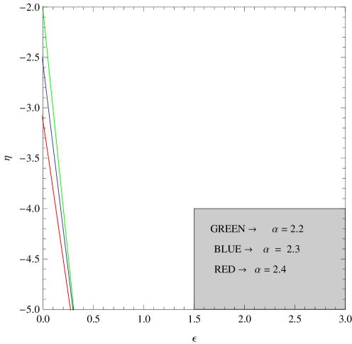
Figure 18: The variation of $\eta$ against $\epsilon$ from (95) and (96) for $A=1,\omega_{b}=.2,\rho_{0}=5,\delta=.5$ and $\alpha=2.2,2.3,2.4$

Fig. 17 shows the variation of $V$ against $\phi$. It has been seen that $V$ decreases as $\phi$ increases. Also from fig. 18, it has been seen that $\eta$ decreases as $\epsilon$ increases.

Case II:

In case of Intermediate Scenario, using (14), equation (90) reduces to,

$$\rho_{b}=\rho_{0}\exp(-3B(1+\omega_{b}-\delta)t^{\beta})$$ (97)

Hence the energy density of the tachyonic fluid is,

$$\rho_{t}=3B^{2}\beta^{2}t^{2\beta-2}-\rho_{0}x_{8}$$ (98)

where, $x_{8}=\exp(-3B(1+\omega_{b}-\delta)t^{\beta})$. Hence the pressure of the tachyonic fluid is,

$$p_{t}=-3B^{2}\beta^{2}t^{2\beta-2}-2B\beta(\beta-1)t^{\beta-2}-\rho_{0}\omega_{b}x_{8}$$ (99)

Solving the equations the tachyonic field and the tachyonic potential are obtained as,

$$\phi=\int\sqrt{\frac{2B\beta(\beta-1)t^{\beta-2}+\rho_{0}\omega_{b}x_{8}}{\rho_{0}x_{8}-3B^{2}\beta^{2}t^{2\beta-2}}}dt$$ (100)

and

$$V(\phi)=\sqrt{3B^{2}\beta^{2}t^{2\beta-2}-\rho_{0}x_{8}}\times\sqrt{3B^{2}\beta^{2}t^{2\beta-2}+2B\beta(\beta-1)t^{\beta-2}+\rho_{0}\omega_{b}x_{8}}$$ (101)

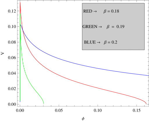
Figure 19: The variation of $V$ against $\phi$ from (100) and (101) for $B=1,\omega_{b}=.3,\rho_{0}=5,\delta=.2$ and $\beta=0.18,0.19,0.2$

The slow-roll parameters will be,

$$\epsilon=2\left(\frac{\beta-1}{t}\right)^{2}\times\frac{\rho_{0}x_{8}-3B^{2}\beta^{2}t^{2\beta-2}}{2B\beta(\beta-1)t^{\beta-2}+\rho_{0}\omega_{b}x_{8}}$$ (102)

and

$$\eta=\frac{2(\beta-1)(\beta-2)}{t^{2}}\times\frac{\rho_{0}x_{8}-3B^{2}\beta^{2}t^{2\beta-2}}{2B\beta(\beta-1)t^{\beta-2}+\rho_{0}\omega_{b}x_{8}}-\left(\frac{\beta-1}{t}\right)\times$$

$$\left(\frac{\rho_{0}x_{8}-3B^{2}\beta^{2}t^{2\beta-2}}{2B\beta(\beta-1)t^{\beta-2}+\rho_{0}\omega_{b}x_{8}}\right)^{2}\times\frac{\partial}{\partial{t}}\left[\frac{2B\beta(\beta-1)t^{\beta-2}+\rho_{0}\omega_{b}x_{8}}{\rho_{0}x_{8}-3B^{2}\beta^{2}t^{2\beta-2}}\right]$$ (103)

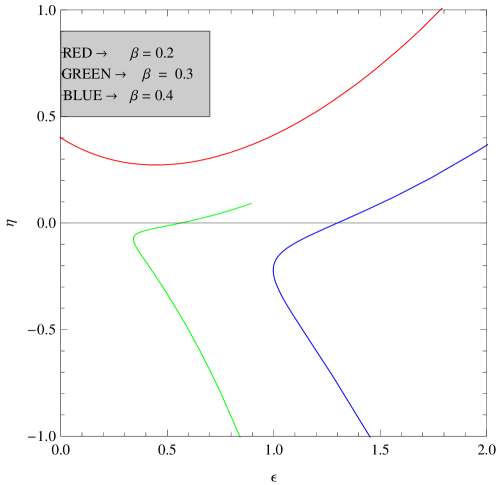
Figure 20: The variation of $\eta$ against $\epsilon$ from (102) and (103) for $B=1,\omega_{b}=.3,\rho_{0}=5,\delta=.2$ and $\beta=0.2,0.3,0.4$

Fig. 19 shows the variation of $V$ against $\phi$. It has been seen that $V$ decreases as $\phi$ increases. Also fig. 20 describes the variation of $\eta$ against $\epsilon$.

V Mixture of Generalized Chaplygin Gas and Barotropic Fluid with Tachyonic Field

Let us consider the universe is filled with the mixture of generalized Chaplygin Gas, barotropic fluid and tachyonic field. This generalized Chaplygin Gas is considered a perfect fluid is given by,

$$p_{c}=-C/{\rho}_{c}^{\gamma}~{}~{},~{}~{}~{}0\leq\gamma\leq 1,C>0.$$ (104)

and the EOS of the barotropic fluid is given by,

$$p_{b}=\omega_{b}\rho_{b}$$ (105)

If the energy density of the fluid is a function of volume only, the temperature of the fluid remains zero at any pressure or volume, violating the third law of thermodynamics. The total energy density and pressure are respectively given by,

$$\rho_{tot}=\rho_{c}+\rho_{b}+\rho_{t}$$ (106)

and

$$p_{tot}=p_{c}+p_{b}+p_{t}$$ (107)

where $p_{c}$ and $\rho_{c}$ are the pressure and density of the generalized Chaplygin gas respectively and $p_{b}$ and $\rho_{b}$ are the pressure and density of the barotropic fluid respectively and $p_{t}$ and $\rho_{t}$ are the pressure and density of the tachyonic field respectively. Now we consider two possible states: (i) without interaction and (ii) with interaction.

V.1 Without Interaction

The energy conservation equation is,

$$\dot{\rho}_{tot}+3\frac{\dot{a}}{a}(\rho_{tot}+p_{tot})=0$$ (108)

Suppose the fluids do not interact with each other. Then the above equation may be written as,

$$\dot{\rho}_{c}+3\frac{\dot{a}}{a}(\rho_{c}+p_{c})=0$$ (109)

$$\dot{\rho}_{b}+3\frac{\dot{a}}{a}(\rho_{b}+p_{b})=0$$ (110)

and

$$\dot{\rho}_{t}+3\frac{\dot{a}}{a}(\rho_{t}+p_{t})=0$$ (111)

Now from equations (104) and (109), after eliminating $p_{c}$ we get $\rho_{c}$ in terms of the scale factor,

$$\rho_{c}=\left[C+\rho_{c}^{\prime}a^{-3(1+\gamma)}\right]^{\frac{1}{1+\gamma}}$$ (112)

and from (105) and (110) we get,

$$\rho_{b}=\rho_{b}^{\prime}~{}a^{-3(1+\omega_{b})}$$ (113)

where $\rho_{c}^{\prime}$ and $\rho_{b}^{\prime}$ are the integrating constants.

From (106), (112) and (113) we get,

$$\rho_{t}=3H^{2}-\left[C+\rho_{c}^{\prime}a^{-3(1+\gamma)}\right]^{\frac{1}{1+\gamma}}-\rho_{b}^{\prime}~{}a^{-3(1+\omega_{b})}$$ (114)

Thus from (107),(111) and (114) we get,

$$p_{t}=-3H^{2}-2\dot{H}+C\left[C+\rho_{c}^{\prime}a^{-3(1+\gamma)}\right]^{\frac{-\gamma}{1+\gamma}}-\omega_{b}\rho_{b}^{\prime}~{}a^{-3(1+\omega_{b})}$$ (115)

Case I:

In the case of Logamediate Inflation the energy density and the pressure of the tachyonic fluid becomes,

$$\rho_{t}=\frac{3A^{2}\alpha^{2}(\ln t)^{2\alpha-2}}{t^{2}}-[C+\rho_{c}^{\prime}x_{1}]^{\frac{1}{(1+\gamma)}}-\rho_{b}^{\prime}x_{5}$$ (116)

$$p_{t}=-\frac{3A^{2}\alpha^{2}(\ln t)^{2\alpha-2}}{t^{2}}+\frac{2A\alpha(\ln t-\alpha+1)(\ln t)^{\alpha-2}}{t^{2}}+C[C+\rho_{c}^{\prime}x_{1}]^{\frac{-\gamma}{(1+\gamma)}}-\rho_{b}^{\prime}\omega_{b}x_{5}$$ (117)

where, $x_{1}=\exp(-3A(1+\gamma)(\ln t)^{\alpha})$ and $x_{5}=\exp(-3A(1+\omega_{b})(\ln t)^{\alpha})$.

From the equations (27), (28), (116) and (117), the tachyonic field and the tachyonic potential are obtained as,

$$\phi=\int\sqrt{\frac{\frac{2A\alpha(-\ln t+\alpha-1)(\ln t)^{\alpha-2}}{t^{2}}+\rho_{c}^{\prime}x_{1}[C+\rho_{c}^{\prime}x_{1}]^{\frac{-\gamma}{\gamma+1}}+\rho_{b}^{\prime}(1+\omega_{b})x_{5}}{{[C+\rho_{c}^{\prime}x_{1}]^{\frac{1}{\gamma+1}}+\rho_{b}^{\prime}x_{5}}-\frac{3A^{2}\alpha^{2}(\ln t)^{2\alpha-2}}{t^{2}}}}~{}dt$$ (118)

and

$$V(\phi)=\sqrt{\frac{3A^{2}\alpha^{2}(\ln t)^{2\alpha-2}}{t^{2}}-[C+\rho_{c}^{\prime}x_{1}]^{\frac{1}{(1+\gamma)}}-\rho_{b}^{\prime}x_{5}}~{}~{}\times~{}~{}~{}~{}~{}~{}~{}~{}~{}~{}~{}~{}~{}~{}~{}~{}~{}~{}~{}~{}~{}~{}~{}~{}~{}~{}$$

$$\sqrt{\frac{3A^{2}\alpha^{2}(\ln t)^{2\alpha-2}}{t^{2}}-\frac{2A\alpha(\ln t-\alpha+1)(\ln t)^{\alpha-2}}{t^{2}}-C[C+\rho_{c}^{\prime}x_{1}]^{\frac{-\gamma}{(1+\gamma)}}+\rho_{b}^{\prime}\omega_{b}x_{5}}$$ (119)

From (7), (8), (29), (30) and (118) we get the slow-roll parameters,

$$\epsilon=2\left(\frac{\alpha-1-\ln t}{t\ln t}\right)^{2}\times\frac{{[C+\rho_{c}^{\prime}x_{1}]^{\frac{1}{\gamma+1}}+\rho_{b}^{\prime}x_{5}}-\frac{3A^{2}\alpha^{2}(\ln t)^{2\alpha-2}}{t^{2}}}{\frac{2A\alpha(-\ln t+\alpha-1)(\ln t)^{\alpha-2}}{t^{2}}+\rho_{c}^{\prime}x_{1}[C+\rho_{c}^{\prime}x_{1}]^{\frac{-\gamma}{\gamma+1}}+\rho_{b}^{\prime}(1+\omega_{b})x_{5}}$$ (120)

and

$$\eta=2\times\frac{{[C+\rho_{c}^{\prime}x_{1}]^{\frac{1}{\gamma+1}}+\rho_{b}^{\prime}x_{5}}-\frac{3A^{2}\alpha^{2}(\ln t)^{2\alpha-2}}{t^{2}}}{\frac{2A\alpha(-\ln t+\alpha-1)(\ln t)^{\alpha-2}}{t^{2}}+\rho_{c}^{\prime}x_{1}[C+\rho_{c}^{\prime}x_{1}]^{\frac{-\gamma}{\gamma+1}}+\rho_{b}^{\prime}(1+\omega_{b})x_{5}}\times\left(\frac{2(\ln t)^{2}-3(\alpha-1)\ln t+(\alpha-1)(\alpha-2)}{t^{2}(\ln t)^{2}}\right)-$$

$$\left(\frac{\alpha-1-\ln t}{t\ln t}\right)\left(\frac{{[C+\rho_{c}^{\prime}x_{1}]^{\frac{1}{\gamma+1}}+\rho_{b}^{\prime}x_{5}}-\frac{3A^{2}\alpha^{2}(\ln t)^{2\alpha-2}}{t^{2}}}{\frac{2A\alpha(-\ln t+\alpha-1)(\ln t)^{\alpha-2}}{t^{2}}+\rho_{c}^{\prime}x_{1}[C+\rho_{c}^{\prime}x_{1}]^{\frac{-\gamma}{\gamma+1}}+\rho_{b}^{\prime}(1+\omega_{b})x_{5}}\right)^{2}$$

$$\frac{\partial}{\partial{t}}\left[\frac{\frac{2A\alpha(-\ln t+\alpha-1)(\ln t)^{\alpha-2}}{t^{2}}+\rho_{c}^{\prime}x_{1}[C+\rho_{c}^{\prime}x_{1}]^{\frac{-\gamma}{\gamma+1}}+\rho_{b}^{\prime}(1+\omega_{b})x_{5}}{{[C+\rho_{c}^{\prime}x_{1}]^{\frac{1}{\gamma+1}}+\rho_{b}^{\prime}x_{5}}-\frac{3A^{2}\alpha^{2}(\ln t)^{2\alpha-2}}{t^{2}}}\right]$$ (121)

Case II:

In case of Intermediate Scenario, the energy density and the pressure of the tachyonic fluid is,

$$\rho_{t}=3B^{2}\beta^{2}t^{2\beta-2}-[C+\rho_{c}^{\prime}x_{2}]^{\frac{1}{(1+\gamma)}}-\rho_{b}^{\prime}x_{6}$$ (122)

and

$$p_{t}=-3B^{2}\beta^{2}t^{2\beta-2}-2B\beta(\beta-1)t^{\beta-2}+C[C+\rho_{0}x_{2}]^{\frac{-\gamma}{(1+\gamma)}}-\rho_{b}^{\prime}\omega_{b}x_{6}$$ (123)

where, $x_{2}=\exp(-3B(1+\gamma)t^{\beta})$ and $x_{6}=\exp(-3B(1+\omega_{b})t^{\beta})$.

Thus the tachyonic field and the tachyonic potential are obtained as,

$$\phi=\int\sqrt{\frac{2B\beta(\beta-1)t^{\beta-2}-C[C+\rho_{c}^{\prime}x_{2}]^{\frac{-\gamma}{(1+\gamma)}}+\rho_{b}^{\prime}(1+\omega_{b})x_{6}}{[C+\rho_{c}^{\prime}x_{2}]^{\frac{1}{(1+\gamma)}}+\rho_{b}^{\prime}x_{6}-3B^{2}\beta^{2}t^{2\beta-2}}}dt$$ (124)

and

$$V(\phi)=\sqrt{3B^{2}\beta^{2}t^{2\beta-2}-[C+\rho_{c}^{\prime}x_{2}]^{\frac{1}{(1+\gamma)}}-\rho_{b}^{\prime}x_{6}}~{}~{}~{}\times$$

$$\sqrt{-3B^{2}\beta^{2}t^{2\beta-2}-2B\beta(\beta-1)t^{\beta-2}+C[C+\rho_{0}x_{2}]^{\frac{-\gamma}{(1+\gamma)}}-\rho_{b}^{\prime}\omega_{b}x_{6}}$$ (125)

From (16), (17), (29), (30) and (124) we get the slow-roll parameters,

$$\epsilon=2\left(\frac{\beta-1}{t}\right)^{2}\times\frac{[C+\rho_{c}^{\prime}x_{2}]^{\frac{1}{(1+\gamma)}}+\rho_{b}^{\prime}x_{6}-3B^{2}\beta^{2}t^{2\beta-2}}{2B\beta(\beta-1)t^{\beta-2}-C[C+\rho_{c}^{\prime}x_{2}]^{\frac{-\gamma}{(1+\gamma)}}+\rho_{b}^{\prime}(1+\omega_{b})x_{6}}$$ (126)

and

$$\eta=\frac{2(\beta-1)(\beta-2)}{t^{2}}\times\frac{[C+\rho_{c}^{\prime}x_{2}]^{\frac{1}{(1+\gamma)}}+\rho_{b}^{\prime}x_{6}-3B^{2}\beta^{2}t^{2\beta-2}}{2B\beta(\beta-1)t^{\beta-2}-C[C+\rho_{c}^{\prime}x_{2}]^{\frac{-\gamma}{(1+\gamma)}}+\rho_{b}^{\prime}(1+\omega_{b})x_{6}}-$$

$$\left(\frac{\beta-1}{t}\right)\left(\frac{[C+\rho_{c}^{\prime}x_{2}]^{\frac{1}{(1+\gamma)}}+\rho_{b}^{\prime}x_{6}-3B^{2}\beta^{2}t^{2\beta-2}}{2B\beta(\beta-1)t^{\beta-2}-C[C+\rho_{c}^{\prime}x_{2}]^{\frac{-\gamma}{(1+\gamma)}}+\rho_{b}^{\prime}(1+\omega_{b})x_{6}}\right)^{2}$$

$$\frac{\partial}{\partial{t}}\left[\frac{2B\beta(\beta-1)t^{\beta-2}-C[C+\rho_{c}^{\prime}x_{2}]^{\frac{-\gamma}{(1+\gamma)}}+\rho_{b}^{\prime}(1+\omega_{b})x_{6}}{[C+\rho_{c}^{\prime}x_{2}]^{\frac{1}{(1+\gamma)}}+\rho_{b}^{\prime}x_{6}-3B^{2}\beta^{2}t^{2\beta-2}}\right]$$ (127)

V.2 With Interaction

Now we consider an interaction between the tachyonic fluid, GCG and barotropic fluid by introducing an interaction terms as a product of the Hubble parameter and the energy densities of the Chaplygin gas and barotropic fluid. Thus there is an energy flow between the three fluids.

Now the equations of motion corresponding to the tachyonic field, GCG and barotropic fluid are respectively,

$$\dot{\rho}_{t}+3\frac{\dot{a}}{a}(\rho_{t}+p_{t})=-3H\delta\rho_{c}-3H\delta^{\prime}\rho_{b}$$ (128)

$$\dot{\rho}_{c}+3\frac{\dot{a}}{a}(\rho_{c}+p_{c})=3H\delta\rho_{c}$$ (129)

and

$$\dot{\rho}_{b}+3\frac{\dot{a}}{a}(\rho_{b}+p_{b})=3H\delta^{\prime}\rho_{b}$$ (130)

where $\delta$ and $\delta^{\prime}$ are the coupling constant.

From (104) and (129) we get,

$$\rho_{c}=\left[\frac{C}{1-\delta}+\rho_{c}^{\prime\prime}a^{-3(1+\gamma)(1-\delta)}\right]^{\frac{1}{(1+\gamma)}}$$ (131)

and from (105) and (130) we get,

$$\rho_{b}=\rho_{b}^{\prime\prime}~{}a^{-3(1+\omega_{b}-\delta^{\prime})}$$ (132)

where $\rho_{b}^{\prime\prime}$ and $\rho_{c}^{\prime\prime}$ are integrating constant.

Case I:

In case of Logamediate Scenario, from (21),(106),(128),(131),(132) we get the solutions:

$$\rho_{t}=\frac{3A^{2}\alpha^{2}(\ln t)^{2\alpha-2}}{t^{2}}-\left[\frac{C}{1-\delta}+\rho_{c}^{\prime\prime}x_{3}\right]^{\frac{1}{(1+\gamma)}}-\rho_{b}^{\prime\prime}x_{7}$$ (133)

where $x_{3}=\exp(-3A(1-\delta)(1+\gamma)(\ln t)^{\alpha})$ and $x_{7}=\exp(-3A(1+\omega_{b}-\delta^{\prime})(\ln t)^{\alpha})$. Hence the pressure of the tachyonic field becomes,

$$p_{t}=-\frac{3A^{2}\alpha^{2}(\ln t)^{2\alpha-2}}{t^{2}}+\frac{2A\alpha(\ln t-\alpha+1)(\ln t)^{\alpha-2}}{t^{2}}+C\left[\frac{C}{1-\delta}+\rho_{0}x_{3}\right]^{\frac{-\gamma}{(1+\gamma)}}-\rho_{b}^{\prime\prime}\omega_{b}x_{7}$$ (134)

Solving the equations, the tachyonic field is obtained as,

$$\phi=\int\sqrt{\frac{\frac{2A\alpha(\ln t-\alpha+1)(\ln t)^{\alpha-2}}{t^{2}}-\left(\frac{C\delta}{1-\delta}+\rho_{c}^{\prime\prime}x_{3}\right)\left(\frac{C}{1-\delta}+\rho_{c}^{\prime\prime}x_{3}\right)^{\frac{-\gamma}{1+\gamma}}-\rho_{b}^{\prime\prime}(1+\omega_{b})x_{7}}{\frac{3A^{2}\alpha^{2}(\ln t)^{2\alpha-2}}{t^{2}}-\left[\frac{C}{1-\delta}+\rho_{c}^{\prime\prime}x_{3}\right]^{\frac{1}{(1+\gamma)}}-\rho_{b}^{\prime\prime}x_{7}}}~{}dt$$ (135)

Also the potential will be of the form,

$$V(\phi)=\sqrt{\frac{3A^{2}\alpha^{2}(\ln t)^{2\alpha-2}}{t^{2}}-\left[\frac{C}{1-\delta}+\rho_{c}^{\prime\prime}x_{3}\right]^{\frac{1}{(1+\gamma)}}-\rho_{b}^{\prime\prime}x_{7}}~{}~{}\times$$

$$\sqrt{\frac{3A^{2}\alpha^{2}(\ln t)^{2\alpha-2}}{t^{2}}-\frac{2A\alpha(\ln t-\alpha+1)(\ln t)^{\alpha-2}}{t^{2}}-C\left[\frac{C}{1-\delta}+\rho_{c}^{\prime\prime}x_{3}\right]^{\frac{-\gamma}{(1+\gamma)}}+\rho_{b}^{\prime\prime}\omega_{b}x_{7}}$$ (136)

The slow-roll parameters are obtained as

$$\epsilon=2\left(\frac{\alpha-1-\ln t}{t\ln t}\right)^{2}\times\frac{\frac{3A^{2}\alpha^{2}(\ln t)^{2\alpha-2}}{t^{2}}-\left[\frac{C}{1-\delta}+\rho_{c}^{\prime\prime}x_{3}\right]^{\frac{1}{(1+\gamma)}}-\rho_{b}^{\prime\prime}x_{7}}{\frac{2A\alpha(\ln t-\alpha+1)(\ln t)^{\alpha-2}}{t^{2}}-\left(\frac{C\delta}{1-\delta}+\rho_{c}^{\prime\prime}x_{3}\right)\left(\frac{C}{1-\delta}+\rho_{c}^{\prime\prime}x_{3}\right)^{\frac{-\gamma}{1+\gamma}}-\rho_{b}^{\prime\prime}(1+\omega_{b})x_{7}}$$ (137)

and

$$\eta=\frac{\frac{3A^{2}\alpha^{2}(\ln t)^{2\alpha-2}}{t^{2}}-\left[\frac{C}{1-\delta}+\rho_{c}^{\prime\prime}x_{3}\right]^{\frac{1}{(1+\gamma)}}-\rho_{b}^{\prime\prime}x_{7}}{\frac{2A\alpha(\ln t-\alpha+1)(\ln t)^{\alpha-2}}{t^{2}}-\left(\frac{C\delta}{1-\delta}+\rho_{c}^{\prime\prime}x_{3}\right)\left(\frac{C}{1-\delta}+\rho_{c}^{\prime\prime}x_{3}\right)^{\frac{-\gamma}{1+\gamma}}-\rho_{b}^{\prime\prime}(1+\omega_{b})x_{7}}\times\frac{4(\ln t)^{2}-6(\alpha-1)\ln t+2(\alpha-1)(\alpha-2)}{t^{2}(\ln t)^{2}}$$

$$-~{}~{}\left(\frac{\alpha-1-\ln t}{t\ln t}\right)\times\frac{\frac{3A^{2}\alpha^{2}(\ln t)^{2\alpha-2}}{t^{2}}-\left[\frac{C}{1-\delta}+\rho_{c}^{\prime\prime}x_{3}\right]^{\frac{1}{(1+\gamma)}}-\rho_{b}^{\prime\prime}x_{7}}{\frac{2A\alpha(\ln t-\alpha+1)(\ln t)^{\alpha-2}}{t^{2}}-\left(\frac{C\delta}{1-\delta}+\rho_{c}^{\prime\prime}x_{3}\right)\left(\frac{C}{1-\delta}+\rho_{c}^{\prime\prime}x_{3}\right)^{\frac{-\gamma}{1+\gamma}}-\rho_{b}^{\prime\prime}(1+\omega_{b})x_{7}}\times$$

$$\frac{\partial}{\partial{t}}\left[\frac{\frac{2A\alpha(\ln t-\alpha+1)(\ln t)^{\alpha-2}}{t^{2}}-\left(\frac{C\delta}{1-\delta}+\rho_{c}^{\prime\prime}x_{3}\right)\left(\frac{C}{1-\delta}+\rho_{c}^{\prime\prime}x_{3}\right)^{\frac{-\gamma}{1+\gamma}}-\rho_{b}^{\prime\prime}(1+\omega_{b})x_{7}}{\frac{3A^{2}\alpha^{2}(\ln t)^{2\alpha-2}}{t^{2}}-\left[\frac{C}{1-\delta}+\rho_{c}^{\prime\prime}x_{3}\right]^{\frac{1}{(1+\gamma)}}-\rho_{b}^{\prime\prime}x_{7}}\right]$$ (138)

Case II:

In case of Intermediate Scenario, the energy density and the pressure of the tachyonic fluid is,

$$\rho_{t}=3B^{2}\beta^{2}t^{2\beta-2}-\left[\frac{C}{1-\delta}+\rho_{c}^{\prime\prime}x_{4}\right]^{\frac{1}{(1+\gamma)}}-\rho_{b}^{\prime\prime}x_{8}$$ (139)

Hence

$$p_{t}=-3B^{2}\beta^{2}t^{2\beta-2}-2B\beta(\beta-1)t^{\beta-2}-\rho_{c}^{\prime\prime}(1-\delta)(1+\gamma)x_{4}\left[\frac{C}{1-\delta}+\rho_{c}^{\prime\prime}x_{4}\right]^{\frac{-\gamma}{(1+\gamma)}}-\rho_{b}^{\prime\prime}\omega_{b}x_{8}$$ (140)

where $x_{4}=\exp(-3B(1-\delta)(1+\gamma)t^{\beta})$ and $x_{8}=\exp(-3B(1+\omega_{b}-\delta^{\prime})t^{\beta})$.

Thus the tachyonic field and the tachyonic potential are obtained as,

$$\phi=\int\sqrt{\frac{2B\beta(\beta-1)t^{\beta-2}-\left[\frac{C}{1-\delta}+\rho_{c}^{\prime\prime}x_{4}\right]^{\frac{1}{(1+\gamma)}}+\rho_{c}^{\prime\prime}(1-\delta)(1+\gamma)x_{4}\left[\frac{C}{1-\delta}+\rho_{c}^{\prime\prime}x_{4}\right]^{\frac{-\gamma}{(1+\gamma)}}+\rho_{b}^{\prime\prime}\omega_{b}x_{8}}{\left[\frac{C}{1-\delta}+\rho_{c}^{\prime\prime}x_{4}\right]^{\frac{1}{(1+\gamma)}}+\rho_{b}^{\prime\prime}x_{8}-3B^{2}\beta^{2}t^{2\beta-2}}}~{}dt$$ (141)

and

$$V(\phi)=\sqrt{3B^{2}\beta^{2}t^{2\beta-2}-\left[\frac{C}{1-\delta}+\rho_{c}^{\prime\prime}x_{4}\right]^{\frac{1}{(1+\gamma)}}-\rho_{b}^{\prime\prime}x_{8}}~{}~{}\times$$

$$\sqrt{3B^{2}\beta^{2}t^{2\beta-2}+2B\beta(\beta-1)t^{\beta-2}+\rho_{c}^{\prime\prime}(1-\delta)(1+\gamma)x_{4}\left[\frac{C}{1-\delta}+\rho_{c}^{\prime\prime}x_{4}\right]^{\frac{-\gamma}{(1+\gamma)}}+\rho_{b}^{\prime\prime}\omega_{b}x_{8}}$$ (142)

The slow-roll parameters will be,

$$\epsilon=2\left(\frac{\beta-1}{t}\right)^{2}\times\frac{\left[\frac{C}{1-\delta}+\rho_{c}^{\prime\prime}x_{4}\right]^{\frac{1}{(1+\gamma)}}+\rho_{b}^{\prime\prime}x_{8}-3B^{2}\beta^{2}t^{2\beta-2}}{2B\beta(\beta-1)t^{\beta-2}-\left[\frac{C}{1-\delta}+\rho_{c}^{\prime\prime}x_{4}\right]^{\frac{1}{(1+\gamma)}}+\rho_{c}^{\prime\prime}(1-\delta)(1+\gamma)x_{4}\left[\frac{C}{1-\delta}+\rho_{c}^{\prime\prime}x_{4}\right]^{\frac{-\gamma}{(1+\gamma)}}+\rho_{b}^{\prime\prime}\omega_{b}x_{8}}$$ (143)

and

$$\eta=\frac{2(\beta-1)(\beta-2)}{t^{2}}\times\frac{\left[\frac{C}{1-\delta}+\rho_{c}^{\prime\prime}x_{4}\right]^{\frac{1}{(1+\gamma)}}+\rho_{b}^{\prime\prime}x_{8}-3B^{2}\beta^{2}t^{2\beta-2}}{2B\beta(\beta-1)t^{\beta-2}-\left[\frac{C}{1-\delta}+\rho_{c}^{\prime\prime}x_{4}\right]^{\frac{1}{(1+\gamma)}}+\rho_{c}^{\prime\prime}(1-\delta)(1+\gamma)x_{4}\left[\frac{C}{1-\delta}+\rho_{c}^{\prime\prime}x_{4}\right]^{\frac{-\gamma}{(1+\gamma)}}+\rho_{b}^{\prime\prime}\omega_{b}x_{8}}$$

$$-\left(\frac{\beta-1}{t}\right)\times\left(\frac{\left[\frac{C}{1-\delta}+\rho_{c}^{\prime\prime}x_{4}\right]^{\frac{1}{(1+\gamma)}}+\rho_{b}^{\prime\prime}x_{8}-3B^{2}\beta^{2}t^{2\beta-2}}{2B\beta(\beta-1)t^{\beta-2}-\left[\frac{C}{1-\delta}+\rho_{c}^{\prime\prime}x_{4}\right]^{\frac{1}{(1+\gamma)}}+\rho_{c}^{\prime\prime}(1-\delta)(1+\gamma)x_{4}\left[\frac{C}{1-\delta}+\rho_{c}^{\prime\prime}x_{4}\right]^{\frac{-\gamma}{(1+\gamma)}}+\rho_{b}^{\prime\prime}\omega_{b}x_{8}}\right)^{2}\times$$

$$\frac{\partial}{\partial{t}}\left[\frac{2B\beta(\beta-1)t^{\beta-2}-\left[\frac{C}{1-\delta}+\rho_{c}^{\prime\prime}x_{4}\right]^{\frac{1}{(1+\gamma)}}+\rho_{c}^{\prime\prime}(1-\delta)(1+\gamma)x_{4}\left[\frac{C}{1-\delta}+\rho_{c}^{\prime\prime}x_{4}\right]^{\frac{-\gamma}{(1+\gamma)}}+\rho_{b}^{\prime\prime}\omega_{b}x_{8}}{\left[\frac{C}{1-\delta}+\rho_{c}^{\prime\prime}x_{4}\right]^{\frac{1}{(1+\gamma)}}+\rho_{b}^{\prime\prime}x_{8}-3B^{2}\beta^{2}t^{2\beta-2}}\right]$$ (144)

VI Discussions

In this work, we have considered a model of two and three component mixture i.e., mixture of Chaplygin gas and barotropic fluid with tachyonic field. In the case, when they have no interaction then both of them retain their own properties. Let us consider an energy flow between barotropic and tachyonic fluids. In both the cases we find the exact solutions for the tachyonic field and the tachyonic potential and show that the tachyonic potential follows the asymptotic behavior. Here the tachyonic field behaves as the dark energy component. For the tachyonic dark matter, GCG is considered as a suitable dark energy model. Later we have also considered an interaction between these two fluids by introducing a coupling term. The coupling function decays with time indicating a strong energy flow at the initial period and weak stable interaction at later stage. To keep the observational support of recent acceleration we have considered two particular forms: (i) Logamediate Scenario (ii) Intermediate Scenario, of evolution of the Universe. In both the scenarios, we have obtained the expressions of statefinder parameters. We graphically show the natures of statefinder parameters for evolution of the universe in both the cases. We have considered the mixture of Chaplygin gas and tachyonic field with and without interactions. Logamediate and intermediate expansions have been considered with and without interaction cases. For all possible cases we have obtained the natures of potentials and slow-roll parameters graphically. Next we have also considered the mixture of barotropic fluid and tachyonic field with and without interactions. Logamediate and intermediate expansions have been considered with and without interaction cases also. For all possible cases we have also obtained the natures of potentials and slow-roll parameters graphically. Finally, we have considered the mixture of tachyonic field, Chaplygin gas and barotropic fluid with and without interactions. Logamediate and intermediate expansions have been considered with and without interaction cases. For all possible cases we have obtained the natures of potentials and slow-roll parameters graphically. Thus the present work shows the natures of statefinder and slow-roll parameters in both logamediate and intermediate scenarios for the evolution of the universe.

References:

$[1]$ N. A. Bachall, J. P. Ostriker, S. Perlmutter and P. J. Steinhardt, Science 284 1481 (1999).
$[2]$ S. J. Perlmutter et al, Astrophys. J. 517 565 (1999).
$[3]$ A. G. Riess et al, Astron. J. 116 1009 (1998).
$[4]$ P. M. Garnavich et al, Astrophys. J. 509 74 (1998).
$[5]$ G. Efstathiou et al, astro-ph/9812226.
$[6]$ B. Ratra and P. J. E. Peebles, Phys. Rev. D 37 3406 (1988).
$[7]$ R. R. Caldwell, R. Dave and P. J. Steinhardt, Phys. Rev. Lett. 80 1582 (1998).
$[8]$ A. Kamenshchik, U. Moschella and V. Pasquier, Phys. Lett. B 511 265 (2001).
$[9]$ V. Gorini, A. Kamenshchik, U. Moschella and V. Pasquier, gr-qc/0403062.
$[10]$ V. Gorini, A. Kamenshchik and U. Moschella, Phys. Rev. D 67 063509 (2003).
$[11]$ U. Alam, V. Sahni , T. D. Saini and A.A. Starobinsky, Mon. Not. Roy. Astron. Soc. 344, 1057 (2003).
$[12]$ M. C. Bento, O. Bertolami and A. A. Sen, Phys. Rev. D 66 043507 (2002).
$[13]$ H. B. Benaoum, hep-th/0205140.
$[14]$ U. Debnath, A. Banerjee and S. Chakraborty, Class. Quantum Grav. 21 5609 (2004).
$[15]$ A. Sen, JHEP 04 048 (2002); JHEP 07 065 (2002); Mod. Phys. Lett. A 17 1797(2002).
$[16]$ J. S. Bagla, H. K. Jassal and T. Padmanabhan, Phys. Rev. D 67 063504 (2003).
$[17]$ E. J. Copeland, M. R. Garousi, M. Sami and S. Tsujikawa, Phys. Rev D 71 043003 (2005).
$[18]$ G. Calcagni and A. R. Liddle, astro-ph/0606003.
$[19]$ E. J. Copeland, M. Sami and S. Tsujikawa, Int. J. Mod. Phys. D 15 1753 (2006).
$[20]$ A. DeBenedictis, A. Das and S. Kloster, Gen. Rel. Grav. 36 2481 (2004).
$[21]$ A. Das, S. Gupta, T. D. Saini and S. Kar, Phys. Rev D 72 043528 (2005).
$[22]$ T. Padmanabhan, Phys. Rev. D 66 021301 R (2002).
$[23]$ M. Sami, Mod. Phys. Lett. A 18 691 (2003).
$[24]$ B. C. Paul and D. Paul, Int. J. Mod. Phys. D 14 1831 (2005).
$[25]$ J. D. Barrow and N. J. Nunes, Phys. Rev. D 76 043501 (2007).
$[26]$ J. D. Barrow, Phys. Lett. B 235 40 (1990); J. D. Barrow and P. Saich, Phys. Lett. B 249 406 (1990); J. D. Barrow, A. R. Liddle, and C. Pahud, Phys. Rev. D 74 127305 (2006).
$[27]$ V. Sahni, T. D. Saini, A. A. Starobinsky and U. Alam, JETP Lett. 77 201 (2003).