Compression-induced failure of electro-active polymeric thin films

Abstract

The insurgence of compression induces wrinkling in actuation devices based on EAPs thin films leading to a sudden decrease of performances up to failure. Based on the classical tension field theory for thin elastic membranes (e.g. [11]), we provide a general framework for the analysis of the insurgence of in-plane compression in membranes of electroactive polymers (EAPs). Our main result is the deduction of a (voltage-dependent) domain in the stretch space which represents tensile configurations. Under the assumption of Mooney-Rivlin materials, we obtain that for growing values of the applied voltage the domain contracts, vanishing at a critical voltage above which the polymer is wrinkled for any stretch configuration. Our approach can be easily implemented in numerical simulations for more complex material behaviors and provides a tool for the analysis of compression instability as a function of the elastic moduli.

The growing interest in electroactive polymers as actuator devices, ranging from medical, biological, robotic, and energy harvesters, results from their qualities such as lightweight, small size, low-cost, flexibility, fast response [8, 7, 3]. A typical device consists of a thin sheet of electroactive polymer sandwiched between two compliant electrodes. The simple mechanism of actuation releases on an electromechanical coupling of the Coulomb forces acting between the electrodes and the elastic forces inside the layer. The electrostatic forces acting on the sheet faces induce a transversal extension that is used as a mean of actuation.

In this paper we are mainly concerned with compression induced instability phenomena of thin polymeric electroactive films. The technological interest on these phenomena is due to the observation that, aside of purely electric breakage, typical failure mechanisms of EAPs technological applications are induced by sudden loss of equilibrium. This instability is due to the thinness of the layer and the consequent inability of sustaining compressive stress. As a result, the importance of prestraining in improving the actuation properties has been evidenced in several papers, (e.g. [6, 8, 12, 10, 14]), where the authors describe, as predicted by our theory, the existence of optimal prestretch values. A theoretical analysis of the insurgence of deformation localization in a variational framework was recently proposed in [4] and [18], and in [13] where the role of damage and dissipation were also analyzed.

Here, we obtain explicit analytical results for Mooney-Rivlin incompressible materials, evaluating the insurgence of compressive instability for a generic membrane . While analytical and numerical results about this phenomenon were already obtained in other articles (see [4], [12] and references therein) under restrictive assumptions on the homogeneity of deformation and on the device geometry, a general analytical approach to this topic is still not available up to the knowledge of the authors.

Our results take inspiration on the tension field theory for elastic membranes ([11], [15], [16]). The main ingredient of the theory is the existence of a natural width, assigning a threshold of one of the in-plane stretches as a function of the other one. This threshold separates compressed and tensile states. Accordingly, in the quoted papers it is shown the possibility of decomposing the stretch space into a domain characterized by positive principal stresses (tensile configurations), a region where one stress is positive and the other is negative (wrinkled configurations), and the remaining region where both stresses are negative.

Here we extend these results to the analysis of electroactivated membranes. As we show, for sufficiently high values of the assigned voltage, the tensile region reduces to an “island”, that we can analytically describe and that shrinks as the voltage is increased. We then deduce the existence of a loading threshold (critical voltage), such that for larger value of the electric load no tensile configuration is possible. The amplitude of the safe stretch region and the critical threshold strongly depend on the constitutive properties of the material: “stiffer” materials are safer.

We point out that our approach can be extended to general constitutive hypotheses. Moreover, our paper does not assume homogeneous deformations and delivers a framework to describe general boundary value problems for thin films of electroactivated materials. We believe that the proposed approach will be useful not only to clearly understand the insurgence of wrinkled configurations and the possible disappearance of stable equilibrium states, but also because it delivers an instrument to study the behavior regarding the compression instability as a function of material moduli. This aspect is fundamental in the field of the design of new electroactive materials, a very active area of scientific and technological research.

To show the ability of the model of putting the subject in the right perspective and clearly describe the physical ingredients of the phenomenon, at the end of the paper we deliver two specific applications to simple boundary value problems amenable of fully analytical results.

1 Preliminary notions

We here collect the main equations for a continuum body under electromechanical loading. We refer the reader to [2] and to the references therein for details.

Let f be the deformation carrying the continuum body $\cal B$ (reference configuration) to the current configuration $\cal B^{\prime}=\textbf{\emph{f}}(\cal B)$. We denote by $\textbf{F}=\nabla\textbf{\emph{f}}$ the deformation gradient, by $\textbf{B}=\textbf{F}\textbf{F}^{T}$ the left Cauchy-Green tensor, and by ${\textbf{\emph{e}}}_{i}$ and $\lambda^{2}_{i}$ the eigenvectors and eigenvalues of B, where the $\lambda_{i}$ are the principal stretches. D and E are the electric displacement and the electric field in the current configuration $\cal B^{\prime}$, respectively. For a linear, homogeneous and isotropic dielectric materials $\textbf{\emph{D}}=\varepsilon\textbf{\emph{E}}$ where $\varepsilon=\varepsilon_{o}\varepsilon_{d}$ with $\varepsilon_{0}$ the permittivity of free space and $\varepsilon_{d}$ the dielectric constant of the material.

The (current) Cauchy stress tensor T in the case of electromechanical body can be decomposed as the sum of the elastic stress tensor $\textbf{T}^{{el}}$ and of the electric Maxwell stress tensor $\textbf{T}^{\tiny\mbox{\it M}}$:

$$\textbf{T}=\textbf{T}^{el}+\textbf{T}^{\tiny\mbox{\it M}}.$$

We consider an incompressible, isotropic, elastic materials, for which $\det\textbf{F}=\lambda_{1}\lambda_{2}\lambda_{3}=1$ and the elastic stress can be represented as a function of B (e.g. [17] Eq.(49.5)) as follows:

$$\begin{array}[]{ccl}\textbf{T}^{el}&=&-\pi\textbf{I}+\beta_{1}(\lambda_{1},\lambda_{2})\textbf{B}+\beta_{2}(\lambda_{1},\lambda_{2})\textbf{B}^{-1}\\ T^{el}_{ij}&=&-\pi\delta_{ij}+\beta_{1}(\lambda_{1},\lambda_{2})B_{ij}+\beta_{2}(\lambda_{1},\lambda_{2})B_{ij}^{-1},\end{array}$$ (1)

where $\beta_{1}$ and $\beta_{2}$ are the response functions and $\pi$ is an undetermined Lagrange multiplier which represents the reactive stress arising by the incompressibility constraint.

The electric part of the stress (Maxwell stress) can be expressed by (see again [2])

$$\begin{array}[]{l}\textbf{T}^{\tiny\mbox{\it M}}=\varepsilon(\textbf{\emph{E}}\otimes\textbf{\emph{E}}-\frac{1}{2}(\textbf{\emph{E}}\cdot\textbf{\emph{E}})\textbf{I}),\vspace{0.2 cm}\\ T^{\tiny\mbox{\it M}}_{ij}=\displaystyle\varepsilon(E_{i}E_{j}-\frac{E^{2}}{2}\delta_{ij}),\end{array}$$ (2)

where $E=|\textbf{\emph{E}}|$. With these positions and without loss of generality, the total current stress in an incompressible, isotropic elastic and dielectrically homogeneous body can be expressed as

$$\begin{array}[]{ccl}\textbf{T}&=&-p\,\textbf{I}+\beta_{1}(\lambda_{1},\lambda_{2})\textbf{B}+\beta_{2}(\lambda_{1},\lambda_{2})\textbf{B}^{-1}+\varepsilon\textbf{\emph{E}}\otimes\textbf{\emph{E}}\\ T_{ij}&=&-p\,\delta_{ij}+\beta_{1}(\lambda_{1},\lambda_{2})B_{ij}+\beta_{2}(\lambda_{1},\lambda_{2})B_{ij}^{-1}+\varepsilon E_{i}E_{j},\end{array}$$ (3)

having set $p=\displaystyle\pi+\frac{\varepsilon}{2}E^{2}$. Thus, the principal stresses have the values

$$t_{i}=T_{ii}=-p+\beta_{1}(\lambda_{1},\lambda_{2})\lambda_{i}^{2}+\beta_{2}(\lambda_{1},\lambda_{2})\lambda_{i}^{-2}+\varepsilon E_{i}^{2}.$$ (4)

2 Tensile stretches region

Consider a thin elastic sheet which is made of isotropic, incompressible material, whose upper and lower faces are bonded to compliant electrodes. The reference configuration is a stress free state with zero applied voltage; we here assume that this configuration coincides with a right cylindrical region with flat mid-surface $\Omega$ and constant thickness $h$. Under the assumption that $h$ is small as compared with $\Omega$ ‘diameter’, we embrace the membrane approximation which asserts that the bending stiffness is zero and that any in-plane compressive stress immediately leads to the membrane buckling, with the appearance of wrinkled regions.

According with most common application schemes of EAPs we assume that $\Omega$ remains flat after deformation. We also assume that orthogonal fibers to the plane of $\Omega$ remain orthogonal to this plane also after deformation. We consider thickness variations that, by the incompressibility hypothesis, are accomplished by compatible variations of the in-plane stretches, so that

$$\lambda_{3}=\frac{1}{\lambda_{1}\lambda_{2}}$$ (5)

where $\textbf{\emph{e}}_{3}$ is the unit vector orthogonal to $\Omega$.

The application of a voltage on the electrodes determines the insurgence of an electric field E which should be rigorously calculated by solving the corresponding electromechanical equilibrium problem (see e.g. [2]). On the other hand, since each electrode is an equipotential surface, coherently with the assumption of preservation of the direction of normal fibers and of membrane thinness, we assume that the electric field remains perpendicular to $\Omega$. Of course this hypothesis fails at the boundary of the membrane and in correspondence with possible deformation localization, but typically, with the hypothesis of small thickness, this approximation can be energetically justified (e.g. [9]). Under the described assumptions, if a voltage $V$ is applied to the electrodes, then the electric field at any point of the current configuration amounts to

$$\textbf{\emph{E}}=\frac{V}{h\lambda_{3}}\textbf{\emph{e}}_{3}.$$ (6)

While the approach that we consider in the following is general, to fix the ideas, we here consider a diffuse constitutive assumption for polymeric materials, i.e. the Mooney-Rivlin constitutive model, characterized by constant response functions:

$$\beta_{1}=2c_{1},\hskip 10.0pt\beta_{2}=-2c_{2},$$ (7)

with $c_{1}\geq 0$ and $c_{2}\geq 0$. It is easy to check that for this material class the shear modulus is given by $\mu=2(c_{1}+c_{2})$, which means that stiffer materials are endowed of higher values of the constants $c_{1}$ and $c_{2}$.

Under these hypotheses (4) gives

$$\begin{array}[]{ccl}t_{1}&=&-p+2c_{1}\lambda_{1}^{2}-2c_{2}\lambda_{1}^{-2}\vspace{0.2 cm}\\ t_{2}&=&-p+2c_{1}\lambda_{2}^{2}-2c_{2}\lambda_{2}^{-2}\vspace{0.2 cm}\\ t_{3}&=&-p+2c_{1}\lambda_{1}^{-2}\lambda_{2}^{-2}+2(k_{\mbox{\tiny{\it V}}}-c_{2})\lambda_{1}^{2}\lambda_{2}^{2}.\\ \end{array}$$ (8)

Here, as proposed in [4], we introduce

$$k_{\mbox{\tiny{\it V}}}=\frac{\varepsilon V^{2}}{2h^{2}}$$ (9)

measuring the electric energy density and representing our activation parameter.

The undetermined multiplier $p$ can be deduced by imposing the boundary condition $t_{3}=0$ on the upper and lower faces:

$$p=2c_{1}\lambda_{1}^{-2}\lambda_{2}^{-2}+2(k_{\mbox{\tiny{\it V}}}-c_{2})\lambda_{1}^{2}\lambda_{2}^{2}.$$ (10)

After substitution in Eq.s (8), the in-plane principal stresses are given by

$$\begin{array}[]{ccl}t_{1}&=&2[c_{1}(\lambda_{1}^{2}-\lambda_{1}^{-2}\lambda_{2}^{-2})-c_{2}(\lambda_{1}^{-2}-\lambda_{1}^{2}\lambda_{2}^{2})-k_{\mbox{\tiny{\it V}}}\lambda_{1}^{2}\lambda_{2}^{2}]\vspace{0.2 cm}\\ t_{2}&=&2[c_{1}(\lambda_{2}^{2}-\lambda_{1}^{-2}\lambda_{2}^{-2})-c_{2}(\lambda_{2}^{-2}-\lambda_{1}^{2}\lambda_{2}^{2})-k_{\mbox{\tiny{\it V}}}\lambda_{1}^{2}\lambda_{2}^{2}].\end{array}$$ (11)

Figure 1: Scheme of the natural strain and membrane wrinkling.

We are now in position to introduce the central idea of natural width in simple tension, first formulated by Pipkin in his seminal work [11] and later developed within the context of Tension Field Theory of thin elastic membranes (e.g., among many others, [15], [16]).

Consider a state of local uniaxial stress in direction (say) $\textbf{\emph{e}}_{1}$; under the assumption $t_{2}=t_{3}=0$, the transverse stretch in direction $\textbf{\emph{e}}_{2}\perp\textbf{\emph{e}}_{1}$ assumes a specific value called natural width in tension, which is constitutively dependent on the stretch $\lambda_{1}$ in direction $\textbf{\emph{e}}_{1}$

$$\lambda_{2}=\nu(\lambda_{1},k_{v}).$$ (12)

Since for $\lambda_{2}=\nu(\lambda_{1},k_{v})$ it is $t_{2}=0$, any attempt to reduce the transverse stretch under this value requires a the application of a compressive stress, leading to the formation of wrinkles (see Fig.1). This hypothesis of the tension field theory (see [16]) on the material behavior can be easily shown to hold in the case here considered of Mooney-Rivlin materials.

While in the classical tension field theory, without electric field, it results $\lambda_{2}=\nu(\lambda_{1})=\lambda_{1}^{-1/2}$, in the present case the natural width depends on the applied voltage and in view of Eq. (11)₂ takes the form

$$\lambda_{2}=\nu(\lambda_{1},k_{v})=\lambda_{1}^{-1/2}\left[\frac{c_{1}+c_{2}\lambda_{1}^{2}}{c_{1}+c_{2}\lambda_{1}^{2}-k_{\mbox{\tiny{\it V}}}\lambda_{1}^{2}}\right]^{1/4}.$$ (13)

Analogous considerations hold for uniaxial tension in direction $\textbf{\emph{e}}_{2}$, so that the condition $t_{1}=0$ gives the natural width in the transverse direction $\textbf{\emph{e}}_{1}$

$$\lambda_{1}=\nu(\lambda_{2},k_{v})=\lambda_{2}^{-1/2}\left[\frac{c_{1}+c_{2}\lambda_{2}^{2}}{c_{1}+c_{2}\lambda_{2}^{2}-k_{\mbox{\tiny{\it V}}}\lambda_{2}^{2}}\right]^{1/4}.$$ (14)

As a consequence we have that: for any given voltage $V$, the membrane is in traction when $\lambda_{1}>\nu(\lambda_{2},k_{v})$ and $\lambda_{2}>\nu(\lambda_{1},k_{v})$. In all other cases, the membrane undergoes a compression-induced instability.

In other words we deduce the existence of a voltage-dependent region in the principal stretches space (see Fig.2)

$$\mathscr{D}(k_{v})=\left\{(\lambda_{1},\lambda_{2}):\lambda_{1}>\nu(\lambda_{2},k_{v}),\hskip 5.0pt\lambda_{2}>\nu(\lambda_{1},k_{v})\right\}$$ (15)

that collects the possible values of $(\lambda_{1},\lambda_{2})$ corresponding to tensile states. Wrinkling arises for combinations of the principal stretches which do not belong to $\mathscr{D}$. The two boundaries of $\mathscr{D}$ represent the states with $t_{1}=0$ or $t_{2}=0$, whereas the two vertexes represent the equibiaxial configurations with $t_{1}=t_{2}=0$.

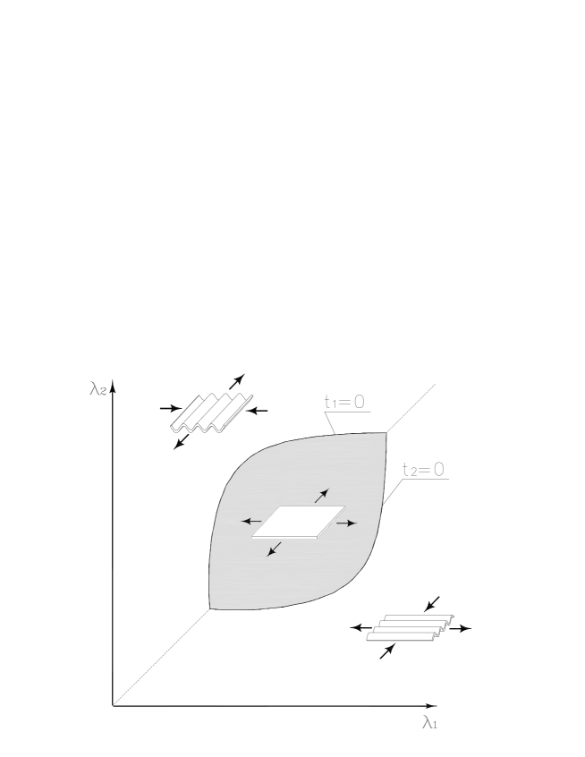
$$\hskip 56.9055pt\mathscr{D}$$

Figure 2: Region $\mathscr{D}$ of tensile states.

Observe that the two curves of the boundary are symmetric with respect to the line $\lambda_{1}=\lambda_{2}$. Thus in the following we restrict our attention to the curve $t_{2}=0$ for $\lambda_{1}>\lambda_{2}$. When the applied voltage is zero, then $\nu(\lambda_{1},0)=\lambda_{1}^{-1/2}$. In this case, the domain $\mathscr{D}$ is unbounded. The application of a voltage modifies the domain $\mathscr{D}$ as follows (see Fig.3). Since $c_{1}\geq 0$ and $c_{2}\geq 0$, a straightforward analysis shows that for $k_{\mbox{\tiny{\it V}}}<c_{2}$ the domain $\mathscr{D}$ remains unbounded, whereas the boundary edges are shifted away from the origin.

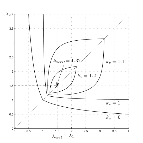
Figure 3: Dependence of the tensile region $\mathscr{D}$ on the activation parameter $k_{v}$. Here for $c_{1}=1$ and $c_{2}=1$. The critical values $k_{v}^{crit}$ and $\lambda^{crit}$ are the activtion thresholds leading to the disappearance of tensile states.

As soon as the voltage overcomes the threshold $k_{\mbox{\tiny{\it V}}}=c_{2}$, the function $\nu$ has a vertical asymptote in correspondence to the stretch

$$\lambda_{1}=\lambda^{*}=\sqrt{\frac{c_{1}}{k_{\mbox{\tiny{\it V}}}-c_{2}}}.$$ (16)

A simple analysis now reveals that for lower values of the voltage parameter $k_{\mbox{\tiny{\it V}}}$ the two symmetric boundary curves of the domain $\mathscr{D}$ intersect at the upper and lower vertexes corresponding to stretches $\lambda_{1}=\lambda_{2}>1$ and $\lambda_{1}=\lambda_{2}<\lambda^{*}$, respectively.

As we show in Fig.3, by increasing the activation parameter $k_{\mbox{\tiny{\it V}}}$ the two vertexes approach each other until they coalesce and no configuration is tensile.

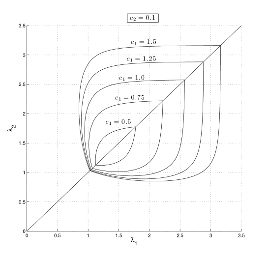
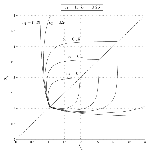
a) b)

Figure 4: Dependence of the tensile region $\mathscr{D}$ on the constitutive parameters $c_{1}$ and $c_{2}$.

We thus deduce the existence of a critical threshold $k_{\mbox{\tiny{\it V}}}=k_{\mbox{\tiny{\it V}}}^{crit}$, such that for $k_{\mbox{\tiny{\it V}}}>k_{\mbox{\tiny{\it V}}}^{crit}$ there is no stable equilibrium configuration. We call $\lambda^{crit}$ the corresponding stretch threshold (see again Fig.3).

We point out that a similar approach can be extended to the more general case of non constant response functions $\beta_{1}=\beta_{1}(\lambda_{1},\lambda_{2})$ and $\beta_{2}=\beta_{2}(\lambda_{1},\lambda_{2})$ with the boundaries of $\mathscr{D}$ obtained by numerically solving $t_{1}=0$ and $t_{2}=0$ in (11). Moreover, we remark that in this analysis we consider only compression induced instabilities, but other types of purely mechanical or electromechanical instabilities can be important (see [13], [18] and [19] and references therein).

Finally, in Fig.4 we show the dependence of the tensile region, for a fixed value of $k_{v}$, on the constitutive parameter $c_{1}$ and $c_{2}$. Observe that in both cases the stiffer is the material, the wider is the region of tensile stretches configurations. It is important to observe that the proposed approach provides an immediate tool for the study of the EAPs behavior regarding compression instability and thus it may reveal its importance in the field of material design.

3 Two simple applications

In this section, as illustrative example, we apply our analysis to homogeneously deformed EAP sheets under different boundary conditions. Despite our approach is not limited by specific constitutive assumptions or boundary conditions, we here take into consideration some simple cases which are amenable of fully analytic solutions and allow an easy interpretation of the results.

Consider firstly the case of Neo-Hookean materials, i.e. $c_{2}=0,c_{1}=\mu/2$, where $\mu$ is the shear modulus. Hence (13) gives

$$\lambda_{2}=\nu(\lambda_{1},k_{\mbox{\tiny{\it V}}})=\lambda_{1}^{-1/2}\left[\frac{\mu}{\mu-2k_{\mbox{\tiny{\it V}}}\lambda_{1}^{2}}\right]^{1/4}.$$ (17)

In this case the two vertexes of the region $\mathscr{D}$, with $\lambda_{1}=\lambda_{2}=\lambda$, are the solutions of

$$2k_{v}\lambda^{8}-\mu\lambda^{6}+\mu=0.$$ (18)

These vertexes coalesce for

$$k_{\mbox{\tiny{\it V}}}=k_{\mbox{\tiny{\it V}}}^{crit}=\frac{3\mu}{2^{\frac{11}{3}}}$$ (19)

which corresponds to an equibiaxial strain

$$\lambda_{1}=\lambda_{2}=\lambda^{crit}=2^{\frac{1}{3}}.$$ (20)

It should be remarked that the simplicity of (19) and (20) is due to the Neo-Hookean constitutive assumption, which is satisfactory only at low stretches. For large stretches the entropic hardening effect, which is not accounted by the Neo-Hookean law, can play an important role in modifying the $\mathscr{D}$ region (see e.g. Fig.4).

We consider now the two following cases, respectively without and with assigned prestretch.

The case without prestretch

Consider first the case of an EAP membrane under an assigned voltage $V$ (see the scheme in Fig.5) and no prestretch at the boundaries. By imposing that $t_{1}=t_{2}=t_{3}=0$ we obtain that the equilibrium solutions correspond to the intersection of $\mathscr{D}$ with the line $\lambda_{1}=\lambda_{2}=\lambda$.

Figure 5: Equilibrium solutions under the hypothesis of homogeneous deformation, in the non prestretched case. Circles represent the equilibrium states for the different values of the activation parameter $k_{v}$.

Thus we are in the case of equibiaxial strain with the in-plane stretch $\lambda$ satisfying Eq. (18). As a consequence we may interpret the vertexes of $\mathscr{D}$ as the stretches corresponding to the present situation. Observe that for given activation $k_{\mbox{\tiny{\it V}}}$ there are two equilibrium solutions. Moreover, the stretch of the equilibrium solution corresponding to the upper vertex decreases as $k_{\mbox{\tiny{\it V}}}$ grows. Thus the thickness of the membrane grows with $k_{\mbox{\tiny{\it V}}}$ so that we may argue that this equilibrium solution is unstable. This is in accordance with the results in [4] where two equilibrium solutions have been obtained for each value of the activation parameter and the larger equilibrium stretch corresponds to an unstable state.

Based on previous analysis, we may deduce that when we increase $k_{\mbox{\tiny{\it V}}}$ there exists a critical value of $k_{\mbox{\tiny{\it V}}}=k_{\mbox{\tiny{\it V}}}^{crit}$ for which the tensile region disappears. This maximum activation value grows with the stiffness of the material. The corresponding limit activation in-plane stretch is given in (20). After this threshold no equilibrium solution is possible. This effect represents what is called in the literature as pull-in instability (see [4]).

The prestretched case

Consider now the hypothesis that a prestretch $\lambda_{2}=\hat{\lambda}_{2}$ is assigned in direction (say) $\textbf{\emph{e}}_{2}$ of a rectangular EAP membrane (see Fig.6). The homogeneous equilibrium solution is obtained by requiring $t_{1}=t_{3}=0$. For given $k_{\mbox{\tiny{\it V}}}$ and $\hat{\lambda}_{2}$, the stretch $\lambda_{1}$ is given by (13) as $\lambda_{1}=\nu(\hat{\lambda}_{2},k_{\mbox{\tiny{\it V}}}$ ). Then we may interpret the boundary of $\mathscr{D}$, i.e. the curves of the natural widths, as representing the equilibrium solutions in the prestretched case.

Observe that the system looses its equilibrium for an activation $k_{\mbox{\tiny{\it V}}}$ (see Fig.6) such that the straight line $\lambda_{1}=\hat{\lambda}_{1}$ corresponds to one of the two vertexes of the tensile region. Thus, the largest activation $k_{\mbox{\tiny{\it V}}}=k_{\mbox{\tiny{\it V}}}^{crit}$ if one chooses a prestretch $\hat{\lambda}_{2}=\lambda^{crit}$. We recall that the existence of an optimal prestretch is also experimentally deduced in [10, 14] and theoretically described in [4] .

Figure 6: Equilibrium solutions under the hypothesis of homogeneous deformation, in the prestretched case. Circles represent the equilibrium states for the different values of the activation parameter $k_{v}$.

Acknowledgment. The authors have been supported by MIUR project PRIN $2008$, ‘Modelli multiscala per strutture in materiali innovativi’ and the project, Progetto di ricerca industriale-Regione Puglia, ‘Modelli innovativi per sistemi meccatronici’.

References

- [1] Beatty F.M., Topics in finite elasticity: Hyperelasticity of rubber, elastomers, and biological tissues – with examples, Appl.Mech.Rev. 40(12), 1699-1734, 1987
- [2] Bustamante R., Dorfman A., Ogden R.W., Nonlinear Electroelastostatics: a variational framework. Z. angew. Math. Phys., 60, 154-177, 2009
- [3] F. Carpi, D. De Rossi, R- Kornbluh, R. Perline, and P. Sommer-Larsen Ed. Dielectric elastomers as electromechanical transducers. Elsevier, 2008.
- [4] D. De Tommasi, G. Puglisi, G. Saccomandi, G. Zurlo. Pull-in and wrinkling instabilities of electroactive dielectric actuators. J. Phys. D: Appl. Phys., 43, 325501., 2010.
- [5] Gurtin M.E., Fried E., Anand L., The Mechanics and Thermodynamics of Continua, Cambridge University Press, 2010.
- [6] G. Kofod. The static actuation of dielectric elastomer actuators: how does pre-stretch improve actuation. J. Phys. D: Appl. Phys., 41, 215405, 2008.
- [7] S. Koh, X. Zhao, and Z. Suo. Maximal energy that can be converted by a dielectric elastomer generator. Appl. Phys. Lett., 94, 262902, 2009.
- [8] R. Kornbluh, R. Perline, Q. Pei, S. Oh, J. Joseph. Ultrahigh strain response of field-actuated elastimeric polymers. Multibody System Dynamics, 1, 149–188, 1997.
- [9] G. W. Parker. Electric field outside a parallel plate capacitor. Am. J. Phys., 70, 502–507, 2002.
- [10] R. Perline, R. Kornbluh, Q. Pei, and J. Joseph. High speed electrically actuated elastomers with strain greater that 100%. Science, 287, 836–839, 2000.
- [11] Pipkin A.C., The Relaxed Energy Density for Isotropic Elastic Membranes, IMA Journal of Applied Mathematics, 40, 85-99, 1986.
- [12] S. Plante, S. Dubowsky. Large-scale Failure modes of dielectric elastomer actuators. Int. J. Sol. Struct., 43, 7727–51, 2006.
- [13] G. Puglisi. Damage localization and stability in electroactive polymers. Report of Mathematisches Forschungsinstitut Oberwolfach, 10, 2008.
- [14] R. Shankar, T.K. Ghosh, R. J. Spontak. Electromechanical response of nanostructured polymer systems with no mechanical pre-Strain. Macromol. Rapid Commun., 28, 1142–1147, 2007.
- [15] Steigmann D.J., Pipkin A.C., Finite Deformations of Wrinkled Membranes, Q.J.Mech.appl.Math. 43(2), 427-440, 1989.
- [16] Steigmann D.J., Tension Field Theory, Proc.R.Soc.Lond. A 429, 141-173,1990
- [17] Truesdell C., Noll W., The Non-Linear Field Theories of Mechanics, Handbuch der Physik III/3 (ed.Flugge) Springer-Verlag Berlin, 1965.
- [18] X. Zhao, W. Hong and Z. Suo. Electromechanical hysteresis and coexistent states in dielectric elastomers. Phys. Rev. B, 76, 134113, 2007.
- [19] X. Zhao and Z. Suo. Electromechanical instability in semicrystalline polymers. Appl. Phys. Lett., 95, 031904, 2009.