Kinetic helicity decay in linearly forced turbulence

Abstract

The decay of kinetic helicity is studied in numerical models of forced turbulence using either an externally imposed forcing function as an inhomogeneous term in the equations or, alternatively, a term linear in the velocity giving rise to a linear instability. The externally imposed forcing function injects energy at the largest scales, giving rise to a turbulent inertial range with nearly constant energy flux while for linearly forced turbulence the spectral energy is maximum near the dissipation wavenumber. Kinetic helicity is injected once a statistically steady state is reached, but it is found to decay on a turbulent time scale regardless of the nature of the forcing and the value of the Reynolds number.

1 Introduction

The physical properties of astrophysical turbulence are often studied by solving the hydrodynamic equations in a periodic domain with an assumed forcing function. In particular, isotropic homogeneous turbulence is often studied as a proxy of turbulence in more complicated situations, where specific concepts and general aspects are harder to isolate. An important concept is that of the forward cascade of kinetic energy to smaller scales. This leads to a $k^{-5/3}$ energy spectrum, where $k$ is the wavenumber. Many flows of geophysical and astrophysical relevance are subject to rotation and stratification and can therefore attain kinetic helicity. Closure calculations ([André & Lesieur 1977]), direct numerical simulations ([Borue & Orszag 1997]; [Brandenburg & Subramanian 2005a]), as well as shell model calculations ([Chkhetiani 1996]; [Ditlevsen & Giuliani 2001a],[b]; [Stepanov et al. 2009]) show an approximate $k^{-5/3}$ scaling for the kinetic helicity, suggesting that kinetic helicity too is subject to a forward cascade toward smaller length scales. On the other hand, kinetic helicity is conserved by the quadratic interactions and might therefore play an important role in the inviscid limit. Although this is also the case in ideal magnetohydrodynamics (MHD), where magnetic helicity is also conserved by the quadratic interactions, there is a significant difference. In the ideal case of small magnetic diffusivity, magnetic helicity can only evolve on resistive time scales. This can have profound effects on the saturation behavior of large-scale dynamos ([Brandenburg 2001]).

As mentioned above, in a polytropic flow, the quadratic interactions conserve kinetic helicity, $\langle\mathchoice{\mbox{\boldmath$\displaystyle\omega$}}{\mbox{\boldmath$\textstyle\omega$}}{\mbox{\boldmath$\scriptstyle\omega$}}{\mbox{\boldmath$\scriptscriptstyle\omega$}}{}\cdot\mathchoice{\mbox{\boldmath$\displaystyle u$}}{\mbox{\boldmath$\textstyle u$}}{\mbox{\boldmath$\scriptstyle u$}}{\mbox{\boldmath$\scriptscriptstyle u$}}{}\rangle$, where $\mathchoice{\mbox{\boldmath$\displaystyle\omega$}}{\mbox{\boldmath$\textstyle\omega$}}{\mbox{\boldmath$\scriptstyle\omega$}}{\mbox{\boldmath$\scriptscriptstyle\omega$}}{}=\mathchoice{\mbox{\boldmath$\displaystyle\nabla$}}{\mbox{\boldmath$\textstyle\nabla$}}{\mbox{\boldmath$\scriptstyle\nabla$}}{\mbox{\boldmath$\scriptscriptstyle\nabla$}}{}\times\mathchoice{\mbox{\boldmath$\displaystyle u$}}{\mbox{\boldmath$\textstyle u$}}{\mbox{\boldmath$\scriptstyle u$}}{\mbox{\boldmath$\scriptscriptstyle u$}}{}$ is the vorticity, $\textstyle u$ the velocity, and angular brackets denote volume averaging over a closed or periodic domain. This conservation property becomes evident when writing the Navier-Stokes equation in the form

$${\partial\mathchoice{\mbox{\boldmath$\displaystyle u$}}{\mbox{\boldmath$\textstyle u$}}{\mbox{\boldmath$\scriptstyle u$}}{\mbox{\boldmath$\scriptscriptstyle u$}}{}\over\partial t}=\mathchoice{\mbox{\boldmath$\displaystyle u$}}{\mbox{\boldmath$\textstyle u$}}{\mbox{\boldmath$\scriptstyle u$}}{\mbox{\boldmath$\scriptscriptstyle u$}}{}\times\mathchoice{\mbox{\boldmath$\displaystyle\omega$}}{\mbox{\boldmath$\textstyle\omega$}}{\mbox{\boldmath$\scriptstyle\omega$}}{\mbox{\boldmath$\scriptscriptstyle\omega$}}{}-\mathchoice{\mbox{\boldmath$\displaystyle\nabla$}}{\mbox{\boldmath$\textstyle\nabla$}}{\mbox{\boldmath$\scriptstyle\nabla$}}{\mbox{\boldmath$\scriptscriptstyle\nabla$}}{}P+\mathchoice{\mbox{\boldmath$\displaystyle f$}}{\mbox{\boldmath$\textstyle f$}}{\mbox{\boldmath$\scriptstyle f$}}{\mbox{\boldmath$\scriptscriptstyle f$}}{}+\nu[{\textstyle{1\over 3}}\mathchoice{\mbox{\boldmath$\displaystyle\nabla$}}{\mbox{\boldmath$\textstyle\nabla$}}{\mbox{\boldmath$\scriptstyle\nabla$}}{\mbox{\boldmath$\scriptscriptstyle\nabla$}}{}(\mathchoice{\mbox{\boldmath$\displaystyle\nabla$}}{\mbox{\boldmath$\textstyle\nabla$}}{\mbox{\boldmath$\scriptstyle\nabla$}}{\mbox{\boldmath$\scriptscriptstyle\nabla$}}{}\cdot\mathchoice{\mbox{\boldmath$\displaystyle u$}}{\mbox{\boldmath$\textstyle u$}}{\mbox{\boldmath$\scriptstyle u$}}{\mbox{\boldmath$\scriptscriptstyle u$}}{})-\mathchoice{\mbox{\boldmath$\displaystyle\nabla$}}{\mbox{\boldmath$\textstyle\nabla$}}{\mbox{\boldmath$\scriptstyle\nabla$}}{\mbox{\boldmath$\scriptscriptstyle\nabla$}}{}\times\mathchoice{\mbox{\boldmath$\displaystyle\nabla$}}{\mbox{\boldmath$\textstyle\nabla$}}{\mbox{\boldmath$\scriptstyle\nabla$}}{\mbox{\boldmath$\scriptscriptstyle\nabla$}}{}\times\mathchoice{\mbox{\boldmath$\displaystyle u$}}{\mbox{\boldmath$\textstyle u$}}{\mbox{\boldmath$\scriptstyle u$}}{\mbox{\boldmath$\scriptscriptstyle u$}}{}+\mathchoice{\mbox{\boldmath$\displaystyle G$}}{\mbox{\boldmath$\textstyle G$}}{\mbox{\boldmath$\scriptstyle G$}}{\mbox{\boldmath$\scriptscriptstyle G$}}{}],$$ (1)

where $P={\textstyle{1\over 2}}\mathchoice{\mbox{\boldmath$\displaystyle u$}}{\mbox{\boldmath$\textstyle u$}}{\mbox{\boldmath$\scriptstyle u$}}{\mbox{\boldmath$\scriptscriptstyle u$}}{}^{2}+h$ is the sum of specific turbulent pressure, $\mathchoice{\mbox{\boldmath$\displaystyle u$}}{\mbox{\boldmath$\textstyle u$}}{\mbox{\boldmath$\scriptstyle u$}}{\mbox{\boldmath$\scriptscriptstyle u$}}{}^{2}/2$, and specific enthalpy, $h=c_{\rm s}^{2}\ln\rho$. Furthermore, $\rho={\rm const}{}$ is the density, and $\textstyle f$ is a forcing function. In the absence of forcing, $\mathchoice{\mbox{\boldmath$\displaystyle f$}}{\mbox{\boldmath$\textstyle f$}}{\mbox{\boldmath$\scriptstyle f$}}{\mbox{\boldmath$\scriptscriptstyle f$}}{}=\bm{0}$, kinetic helicity is just subject to viscous decay, because the nonlinear term $\mathchoice{\mbox{\boldmath$\displaystyle u$}}{\mbox{\boldmath$\textstyle u$}}{\mbox{\boldmath$\scriptstyle u$}}{\mbox{\boldmath$\scriptscriptstyle u$}}{}\times\mathchoice{\mbox{\boldmath$\displaystyle\omega$}}{\mbox{\boldmath$\textstyle\omega$}}{\mbox{\boldmath$\scriptstyle\omega$}}{\mbox{\boldmath$\scriptscriptstyle\omega$}}{}$ is perpendicular to $\textstyle\omega$, i.e., we have

$${{\rm d}{}\over{\rm d}{}t}\langle\mathchoice{\mbox{\boldmath$\displaystyle\omega$}}{\mbox{\boldmath$\textstyle\omega$}}{\mbox{\boldmath$\scriptstyle\omega$}}{\mbox{\boldmath$\scriptscriptstyle\omega$}}{}\cdot\mathchoice{\mbox{\boldmath$\displaystyle u$}}{\mbox{\boldmath$\textstyle u$}}{\mbox{\boldmath$\scriptstyle u$}}{\mbox{\boldmath$\scriptscriptstyle u$}}{}\rangle=-2\nu\langle\mathchoice{\mbox{\boldmath$\displaystyle q$}}{\mbox{\boldmath$\textstyle q$}}{\mbox{\boldmath$\scriptstyle q$}}{\mbox{\boldmath$\scriptscriptstyle q$}}{}\cdot\mathchoice{\mbox{\boldmath$\displaystyle\omega$}}{\mbox{\boldmath$\textstyle\omega$}}{\mbox{\boldmath$\scriptstyle\omega$}}{\mbox{\boldmath$\scriptscriptstyle\omega$}}{}\rangle,$$ (2)

where $\mathchoice{\mbox{\boldmath$\displaystyle q$}}{\mbox{\boldmath$\textstyle q$}}{\mbox{\boldmath$\scriptstyle q$}}{\mbox{\boldmath$\scriptscriptstyle q$}}{}=\mathchoice{\mbox{\boldmath$\displaystyle\nabla$}}{\mbox{\boldmath$\textstyle\nabla$}}{\mbox{\boldmath$\scriptstyle\nabla$}}{\mbox{\boldmath$\scriptscriptstyle\nabla$}}{}\times\mathchoice{\mbox{\boldmath$\displaystyle\omega$}}{\mbox{\boldmath$\textstyle\omega$}}{\mbox{\boldmath$\scriptstyle\omega$}}{\mbox{\boldmath$\scriptscriptstyle\omega$}}{}$ is the curl of the vorticity. In the ideal case, $\nu=0$, we have $\langle\mathchoice{\mbox{\boldmath$\displaystyle\omega$}}{\mbox{\boldmath$\textstyle\omega$}}{\mbox{\boldmath$\scriptstyle\omega$}}{\mbox{\boldmath$\scriptscriptstyle\omega$}}{}\cdot\mathchoice{\mbox{\boldmath$\displaystyle u$}}{\mbox{\boldmath$\textstyle u$}}{\mbox{\boldmath$\scriptstyle u$}}{\mbox{\boldmath$\scriptscriptstyle u$}}{}\rangle={\rm const}{}$. However, in fluid dynamics the ideal case is hardly representative of the limit of large Reynolds numbers, where $\nu\to 0$. Indeed, for a self-similar decay of kinetic energy, the wavenumber of the energy-carrying eddies, $k_{\rm f}$, decreases with time such that $\nu k_{\rm f}^{2}t\approx{\rm const}{}$. This implies that the rate of energy decay, $\nu\langle\mathchoice{\mbox{\boldmath$\displaystyle\omega$}}{\mbox{\boldmath$\textstyle\omega$}}{\mbox{\boldmath$\scriptstyle\omega$}}{\mbox{\boldmath$\scriptscriptstyle\omega$}}{}^{2}\rangle$, is essentially independent of $\nu$ and hence independent of the Reynolds number. Given that $\langle\mathchoice{\mbox{\boldmath$\displaystyle u$}}{\mbox{\boldmath$\textstyle u$}}{\mbox{\boldmath$\scriptstyle u$}}{\mbox{\boldmath$\scriptscriptstyle u$}}{}^{2}\rangle$ is related to the kinetic energy, which is also independent of the Reynolds number, we expect that the ratio

$$\langle\mathchoice{\mbox{\boldmath$\displaystyle\omega$}}{\mbox{\boldmath$\textstyle\omega$}}{\mbox{\boldmath$\scriptstyle\omega$}}{\mbox{\boldmath$\scriptscriptstyle\omega$}}{}^{2}\rangle/\langle\mathchoice{\mbox{\boldmath$\displaystyle u$}}{\mbox{\boldmath$\textstyle u$}}{\mbox{\boldmath$\scriptstyle u$}}{\mbox{\boldmath$\scriptscriptstyle u$}}{}^{2}\rangle\equiv k_{\rm Tay}^{2},$$ (3)

which is related to the Taylor micro-scale wavenumber $k_{\rm Tay}$, should be proportional to Re, and therefore

$$k_{\rm Tay}\sim\mbox{\rm Re}^{1/2}.$$ (4)

However, for helical flows the rate of kinetic helicity dissipation is proportional to $\nu\langle\mathchoice{\mbox{\boldmath$\displaystyle q$}}{\mbox{\boldmath$\textstyle q$}}{\mbox{\boldmath$\scriptstyle q$}}{\mbox{\boldmath$\scriptscriptstyle q$}}{}\cdot\mathchoice{\mbox{\boldmath$\displaystyle\omega$}}{\mbox{\boldmath$\textstyle\omega$}}{\mbox{\boldmath$\scriptstyle\omega$}}{\mbox{\boldmath$\scriptscriptstyle\omega$}}{}\rangle$. Thus, if we define

$$\langle\mathchoice{\mbox{\boldmath$\displaystyle q$}}{\mbox{\boldmath$\textstyle q$}}{\mbox{\boldmath$\scriptstyle q$}}{\mbox{\boldmath$\scriptscriptstyle q$}}{}\cdot\mathchoice{\mbox{\boldmath$\displaystyle\omega$}}{\mbox{\boldmath$\textstyle\omega$}}{\mbox{\boldmath$\scriptstyle\omega$}}{\mbox{\boldmath$\scriptscriptstyle\omega$}}{}\rangle/\langle\mathchoice{\mbox{\boldmath$\displaystyle\omega$}}{\mbox{\boldmath$\textstyle\omega$}}{\mbox{\boldmath$\scriptstyle\omega$}}{\mbox{\boldmath$\scriptscriptstyle\omega$}}{}\cdot\mathchoice{\mbox{\boldmath$\displaystyle u$}}{\mbox{\boldmath$\textstyle u$}}{\mbox{\boldmath$\scriptstyle u$}}{\mbox{\boldmath$\scriptscriptstyle u$}}{}\rangle\equiv k_{\rm eff}^{2},$$ (5)

we see that kinetic helicity dissipation is related to kinetic energy by altogether 3 wavenumber factors. If all these factors scale like in Eq. (4), we may expect the rate of kinetic helicity dissipation to diverge with decreasing $\nu$ like $\nu^{-1/2}$. This is in stark contrast to the related case of magneto-hydrodynamic turbulence where, following similar reasoning, the magnetic helicity dissipation converges to zero like $\eta^{1/2}$ as the magnetic dissipation $\eta$ goes to zero ([Brandenburg & Subramanian 2005b]); see also the appendix of [Brandenburg & Käpylä (2007)] for a clear exposition of these differences.

A problem with the simple argument above is that in cases of practical relevance the forcing function $\textstyle f$ usually breaks kinetic helicity conservation. This is particularly evident for the so-called linear forcing model of [Lundgren (2003)], where

$$\mathchoice{\mbox{\boldmath$\displaystyle f$}}{\mbox{\boldmath$\textstyle f$}}{\mbox{\boldmath$\scriptstyle f$}}{\mbox{\boldmath$\scriptscriptstyle f$}}{}=A\mathchoice{\mbox{\boldmath$\displaystyle u$}}{\mbox{\boldmath$\textstyle u$}}{\mbox{\boldmath$\scriptstyle u$}}{\mbox{\boldmath$\scriptscriptstyle u$}}{}$$ (6)

is a positive multiple of the velocity vector. In that case we have

$${{\rm d}{}\over{\rm d}{}t}\langle\mathchoice{\mbox{\boldmath$\displaystyle\omega$}}{\mbox{\boldmath$\textstyle\omega$}}{\mbox{\boldmath$\scriptstyle\omega$}}{\mbox{\boldmath$\scriptscriptstyle\omega$}}{}\cdot\mathchoice{\mbox{\boldmath$\displaystyle u$}}{\mbox{\boldmath$\textstyle u$}}{\mbox{\boldmath$\scriptstyle u$}}{\mbox{\boldmath$\scriptscriptstyle u$}}{}\rangle=2A\langle\mathchoice{\mbox{\boldmath$\displaystyle\omega$}}{\mbox{\boldmath$\textstyle\omega$}}{\mbox{\boldmath$\scriptstyle\omega$}}{\mbox{\boldmath$\scriptscriptstyle\omega$}}{}\cdot\mathchoice{\mbox{\boldmath$\displaystyle u$}}{\mbox{\boldmath$\textstyle u$}}{\mbox{\boldmath$\scriptstyle u$}}{\mbox{\boldmath$\scriptscriptstyle u$}}{}\rangle-2\nu\langle\mathchoice{\mbox{\boldmath$\displaystyle q$}}{\mbox{\boldmath$\textstyle q$}}{\mbox{\boldmath$\scriptstyle q$}}{\mbox{\boldmath$\scriptscriptstyle q$}}{}\cdot\mathchoice{\mbox{\boldmath$\displaystyle\omega$}}{\mbox{\boldmath$\textstyle\omega$}}{\mbox{\boldmath$\scriptstyle\omega$}}{\mbox{\boldmath$\scriptscriptstyle\omega$}}{}\rangle,$$ (7)

so that $\langle\mathchoice{\mbox{\boldmath$\displaystyle\omega$}}{\mbox{\boldmath$\textstyle\omega$}}{\mbox{\boldmath$\scriptstyle\omega$}}{\mbox{\boldmath$\scriptscriptstyle\omega$}}{}\cdot\mathchoice{\mbox{\boldmath$\displaystyle u$}}{\mbox{\boldmath$\textstyle u$}}{\mbox{\boldmath$\scriptstyle u$}}{\mbox{\boldmath$\scriptscriptstyle u$}}{}\rangle$ could even exhibit exponential growth. An aim of this paper is thus to investigate to what degree kinetic helicity is conserved in forced turbulence using both the linear forcing model and compare it with the more traditional stochastic forcing in a narrow wavenumber band. Another motivation is the fact that, by analogy, magnetic helicity turned out to be of crucial importance in understanding the saturation properties of helically forced dynamos in periodic domains (see, e.g., [Brandenburg 2001]). We study the kinetic helicity evolution by monitoring the response to adding a large-scale helical component to the flow for both types of forcing.

2 Method

In the following we present results obtained by solving the compressible hydrodynamic equations with an imposed random forcing term and an isothermal equation of state, so that the pressure $p$ is related to $\rho$ via $p=\rho c_{\rm s}^{2}$, where $c_{\rm s}$ is the isothermal sound speed. We thus deviate from the conceptually simpler incompressible case. The reason for doing this is that we are mainly interested in astrophysical applications where the gas is compressible. Furthermore, we expect that for small Mach numbers, compressible and incompressible cases become nearly identical. However, this is only partially true, as the zero-Mach number limit may not be uniform and may not commute with the small-scale, long-time or zero-viscosity limits.

In the following we use an isothermal equation of state for a monatomic gas for which the bulk viscosity vanishes, so the hydrodynamic equations for $\rho$ and $\textstyle u$ take the form

$${\partial\rho\over\partial t}=-\mathchoice{\mbox{\boldmath$\displaystyle\nabla$}}{\mbox{\boldmath$\textstyle\nabla$}}{\mbox{\boldmath$\scriptstyle\nabla$}}{\mbox{\boldmath$\scriptscriptstyle\nabla$}}{}\cdot\rho\mathchoice{\mbox{\boldmath$\displaystyle u$}}{\mbox{\boldmath$\textstyle u$}}{\mbox{\boldmath$\scriptstyle u$}}{\mbox{\boldmath$\scriptscriptstyle u$}}{},$$ (8)

$${\partial\mathchoice{\mbox{\boldmath$\displaystyle u$}}{\mbox{\boldmath$\textstyle u$}}{\mbox{\boldmath$\scriptstyle u$}}{\mbox{\boldmath$\scriptscriptstyle u$}}{}\over\partial t}=-\mathchoice{\mbox{\boldmath$\displaystyle u$}}{\mbox{\boldmath$\textstyle u$}}{\mbox{\boldmath$\scriptstyle u$}}{\mbox{\boldmath$\scriptscriptstyle u$}}{}\cdot\mathchoice{\mbox{\boldmath$\displaystyle\nabla$}}{\mbox{\boldmath$\textstyle\nabla$}}{\mbox{\boldmath$\scriptstyle\nabla$}}{\mbox{\boldmath$\scriptscriptstyle\nabla$}}{}\mathchoice{\mbox{\boldmath$\displaystyle u$}}{\mbox{\boldmath$\textstyle u$}}{\mbox{\boldmath$\scriptstyle u$}}{\mbox{\boldmath$\scriptscriptstyle u$}}{}-c_{\rm s}^{2}\mathchoice{\mbox{\boldmath$\displaystyle\nabla$}}{\mbox{\boldmath$\textstyle\nabla$}}{\mbox{\boldmath$\scriptstyle\nabla$}}{\mbox{\boldmath$\scriptscriptstyle\nabla$}}{}\ln\rho+\mathchoice{\mbox{\boldmath$\displaystyle f$}}{\mbox{\boldmath$\textstyle f$}}{\mbox{\boldmath$\scriptstyle f$}}{\mbox{\boldmath$\scriptscriptstyle f$}}{}+\rho^{-1}\mathchoice{\mbox{\boldmath$\displaystyle\nabla$}}{\mbox{\boldmath$\textstyle\nabla$}}{\mbox{\boldmath$\scriptstyle\nabla$}}{\mbox{\boldmath$\scriptscriptstyle\nabla$}}{}\cdot 2\rho\nu\bm{\mathsf{S}},$$ (9)

where ${\sf S}_{ij}={\textstyle{1\over 2}}(u_{i,j}+u_{j,i})-{\textstyle{1\over 3}}\delta_{ij}\mathchoice{\mbox{\boldmath$\displaystyle\nabla$}}{\mbox{\boldmath$\textstyle\nabla$}}{\mbox{\boldmath$\scriptstyle\nabla$}}{\mbox{\boldmath$\scriptscriptstyle\nabla$}}{}\cdot\mathchoice{\mbox{\boldmath$\displaystyle u$}}{\mbox{\boldmath$\textstyle u$}}{\mbox{\boldmath$\scriptstyle u$}}{\mbox{\boldmath$\scriptscriptstyle u$}}{}$ is the traceless rate of strain tensor, $\nu$ is the kinematic viscosity, and $\textstyle f$ is a forcing function that is either given by the linear forcing model using Eq. (6) with a positive constant $A$, or, alternatively, it is given by a random forcing function consisting of plane transversal waves with random wavevectors $\textstyle k$ such that $|\mathchoice{\mbox{\boldmath$\displaystyle k$}}{\mbox{\boldmath$\textstyle k$}}{\mbox{\boldmath$\scriptstyle k$}}{\mbox{\boldmath$\scriptscriptstyle k$}}{}|$ lies in a band around a given forcing wavenumber $k_{\rm f}$. The vector $\textstyle k$ changes randomly from one timestep to the next, so $\textstyle f$ is $\delta$ correlated in time. The forcing amplitude is chosen such that the Mach number, $\mbox{\rm Ma}=u_{\rm rms}/c_{\rm s}$, is about 0.1. Here, $u_{\rm rms}=\langle\mathchoice{\mbox{\boldmath$\displaystyle u$}}{\mbox{\boldmath$\textstyle u$}}{\mbox{\boldmath$\scriptstyle u$}}{\mbox{\boldmath$\scriptscriptstyle u$}}{}^{2}\rangle^{1/2}$ is the root-mean-square (rms) velocity. We use triply-periodic boundary conditions in a Cartesian domain of size $L^{3}$. The smallest wavenumber that fits into the computational domain is $k_{1}=2\pi/L$.

For the linear forcing model we choose for the amplitude $A/c_{\rm s}k_{1}=0.02$, while for the random forcing function, $\textstyle f$ is of the form

$$\mathchoice{\mbox{\boldmath$\displaystyle f$}}{\mbox{\boldmath$\textstyle f$}}{\mbox{\boldmath$\scriptstyle f$}}{\mbox{\boldmath$\scriptscriptstyle f$}}{}(\mathchoice{\mbox{\boldmath$\displaystyle x$}}{\mbox{\boldmath$\textstyle x$}}{\mbox{\boldmath$\scriptstyle x$}}{\mbox{\boldmath$\scriptscriptstyle x$}}{},t)=\mbox{\rm Re}\{N\mathchoice{\mbox{\boldmath$\displaystyle f$}}{\mbox{\boldmath$\textstyle f$}}{\mbox{\boldmath$\scriptstyle f$}}{\mbox{\boldmath$\scriptscriptstyle f$}}{}_{\mathchoice{\mbox{\boldmath$\displaystyle k$}}{\mbox{\boldmath$\textstyle k$}}{\mbox{\boldmath$\scriptstyle k$}}{\mbox{\boldmath$\scriptscriptstyle k$}}{}(t)}\exp[{\rm i}\mathchoice{\mbox{\boldmath$\displaystyle k$}}{\mbox{\boldmath$\textstyle k$}}{\mbox{\boldmath$\scriptstyle k$}}{\mbox{\boldmath$\scriptscriptstyle k$}}{}(t)\cdot\mathchoice{\mbox{\boldmath$\displaystyle x$}}{\mbox{\boldmath$\textstyle x$}}{\mbox{\boldmath$\scriptstyle x$}}{\mbox{\boldmath$\scriptscriptstyle x$}}{}+{\rm i}\phi(t)]\},$$ (10)

$\textstyle x$ is the position vector and

$$\mathchoice{\mbox{\boldmath$\displaystyle f$}}{\mbox{\boldmath$\textstyle f$}}{\mbox{\boldmath$\scriptstyle f$}}{\mbox{\boldmath$\scriptscriptstyle f$}}{}_{\mathchoice{\mbox{\boldmath$\displaystyle k$}}{\mbox{\boldmath$\textstyle k$}}{\mbox{\boldmath$\scriptstyle k$}}{\mbox{\boldmath$\scriptscriptstyle k$}}{}}=\left(\mathchoice{\mbox{\boldmath$\displaystyle k$}}{\mbox{\boldmath$\textstyle k$}}{\mbox{\boldmath$\scriptstyle k$}}{\mbox{\boldmath$\scriptscriptstyle k$}}{}\times\mathchoice{\mbox{\boldmath$\displaystyle e$}}{\mbox{\boldmath$\textstyle e$}}{\mbox{\boldmath$\scriptstyle e$}}{\mbox{\boldmath$\scriptscriptstyle e$}}{}\right)/\sqrt{\mathchoice{\mbox{\boldmath$\displaystyle k$}}{\mbox{\boldmath$\textstyle k$}}{\mbox{\boldmath$\scriptstyle k$}}{\mbox{\boldmath$\scriptscriptstyle k$}}{}^{2}-(\mathchoice{\mbox{\boldmath$\displaystyle k$}}{\mbox{\boldmath$\textstyle k$}}{\mbox{\boldmath$\scriptstyle k$}}{\mbox{\boldmath$\scriptscriptstyle k$}}{}\cdot\mathchoice{\mbox{\boldmath$\displaystyle e$}}{\mbox{\boldmath$\textstyle e$}}{\mbox{\boldmath$\scriptstyle e$}}{\mbox{\boldmath$\scriptscriptstyle e$}}{})^{2}},$$ (11)

where $\textstyle e$ is an arbitrary unit vector not aligned with $\textstyle k$; note that $|\mathchoice{\mbox{\boldmath$\displaystyle f$}}{\mbox{\boldmath$\textstyle f$}}{\mbox{\boldmath$\scriptstyle f$}}{\mbox{\boldmath$\scriptscriptstyle f$}}{}_{\mathchoice{\mbox{\boldmath$\displaystyle k$}}{\mbox{\boldmath$\textstyle k$}}{\mbox{\boldmath$\scriptstyle k$}}{\mbox{\boldmath$\scriptscriptstyle k$}}{}}|^{2}=1$. The wave vector $\mathchoice{\mbox{\boldmath$\displaystyle k$}}{\mbox{\boldmath$\textstyle k$}}{\mbox{\boldmath$\scriptstyle k$}}{\mbox{\boldmath$\scriptscriptstyle k$}}{}(t)$ and the random phase $-\pi<\phi(t)\leq\pi$ change at every time step. For the time-integrated forcing function to be independent of the length of the time step $\delta t$, the normalization factor $N$ has to be proportional to $\delta t^{-1/2}$. On dimensional grounds it is chosen to be $N=f_{0}c_{\rm s}(k_{\rm f}c_{\rm s}/\delta t)^{1/2}$, where $f_{0}$ is a nondimensional forcing amplitude, which is chosen to be $f_{0}=0.02$. For the monochromatically forced simulations we choose $k_{\rm f}=1.5\,k_{1}$. For the linear forcing module, on the other hand, we compute $k_{\rm f}$ is the integral scale from the resulting kinetic energy spectrum (see below).

Our simulations are characterized by the value of the Reynolds number,

$$\mbox{\rm Re}=u_{\rm rms}/\nu k_{\rm f}.$$ (12)

where the wavenumber $k_{\rm f}$ is either the forcing wavenumber in the case of monochromatic random forcing, or it is evaluated as the wavenumber of the energy-carrying eddies,

$$k_{\rm f}^{-1}=\int k^{-1}E(k)\,{\rm d}{}k\left/\int E(k)\,{\rm d}{}k\right.,$$ (13)

with $E(k)$ being the kinetic energy spectrum, which is here normalized such that

$$\int_{0}^{\infty}E(k)\,{\rm d}{}k={\textstyle{1\over 2}}\langle\mathchoice{\mbox{\boldmath$\displaystyle u$}}{\mbox{\boldmath$\textstyle u$}}{\mbox{\boldmath$\scriptstyle u$}}{\mbox{\boldmath$\scriptscriptstyle u$}}{}^{2}\rangle.$$ (14)

It turns out the in the former case of monochromatic random forcing, the definition (13) agrees well with the a priori chosen forcing wavenumber. We plot energy spectra as a function of $k$ in units of the dissipation wavenumber,

$$k_{\rm d}=(\epsilon/\nu^{3})^{1/4}.$$ (15)

Here, $\epsilon=\nu\langle\mathchoice{\mbox{\boldmath$\displaystyle\omega$}}{\mbox{\boldmath$\textstyle\omega$}}{\mbox{\boldmath$\scriptstyle\omega$}}{\mbox{\boldmath$\scriptscriptstyle\omega$}}{}^{2}\rangle$ is the rate of energy dissipation. We also analyze spectra of kinetic helicity, $F(k)$, which are normalized such that

$$\int_{0}^{\infty}F(k)\,{\rm d}{}k=\langle\mathchoice{\mbox{\boldmath$\displaystyle\omega$}}{\mbox{\boldmath$\textstyle\omega$}}{\mbox{\boldmath$\scriptstyle\omega$}}{\mbox{\boldmath$\scriptscriptstyle\omega$}}{}\cdot\mathchoice{\mbox{\boldmath$\displaystyle u$}}{\mbox{\boldmath$\textstyle u$}}{\mbox{\boldmath$\scriptstyle u$}}{\mbox{\boldmath$\scriptscriptstyle u$}}{}\rangle.$$ (16)

We note that the kinetic helicity spectrum can have either sign and its modulus obeys the well-known realizability condition, $|F(k)|\leq 2kE(k)$ ([Moffatt 1969]).

In the statistically steady state, the kinetic helicity fluctuates around zero. We consider the evolution of kinetic helicity after adding an instantaneous finite perturbation in the form of a Beltrami field,

$$\mathchoice{\mbox{\boldmath$\displaystyle u$}}{\mbox{\boldmath$\textstyle u$}}{\mbox{\boldmath$\scriptstyle u$}}{\mbox{\boldmath$\scriptscriptstyle u$}}{}\to\mathchoice{\mbox{\boldmath$\displaystyle u$}}{\mbox{\boldmath$\textstyle u$}}{\mbox{\boldmath$\scriptstyle u$}}{\mbox{\boldmath$\scriptscriptstyle u$}}{}+\epsilon c_{\rm s}(\sin kz,\cos kz,0),$$ (17)

where $\epsilon$ is a nondimensional input parameter. In all cases we choose $k=k_{1}$, i.e., we perturb the system with a wave on the scale of the domain. We express time in units of turnover times, so that $tu_{\rm rms}k_{\rm f}$ is a nondimensional time.

The simulations have been carried out using the Pencil Code which is a high-order finite-difference code (sixth order in space and third order in time) for solving the compressible hydrodynamic equations.

Figure 1: Kinetic energy spectra compensated with $k^{5/3}\epsilon^{-2/3}$ for a range of different Reynolds numbers and numerical resolutions up to $512^{3}$ mesh points.

3 Results

3.1 Linear forcing model

In Fig. 1 we show compensated spectra of kinetic energy for different values of the Reynolds number. The spectra collapse onto each other in the dissipation range if the wavenumber is scaled with $k_{\rm d}$. With increasing Reynolds number the spectra begin to sketch out a continuation toward smaller wavenumber $k$. Note that in the linear forcing model, energy is being injected at all length scales and not just at the largest scale of the domain. This is a property that may also be responsible for the fact that the effective driving scale tends to be smaller than in otherwise equivalent monochromatically forced simulations ([Rosales & Meneveau 2005]).

In the statistically steady state, the kinetic helicity fluctuates around zero. However, after adding a finite perturbation in the form of Eq. (17), the helicity begins to grow for about 5 turnover times, $\delta tu_{\rm rms}k_{\rm f}\approx 5$. After that time there is a systematic decline of the kinetic helicity. By inspecting the results for different values of Re, we see that the time it takes for the kinetic helicity to relax to previous levels becomes longer as the Reynolds number is increased from 44 to 125; see Fig. 2. However, for $\mbox{\rm Re}=300$, which is our largest Reynolds number for which we have performed experiments with added Beltrami fields, the decline of helicity has happened on a similar time scale as for $\mbox{\rm Re}=70$. This suggests that there may not be a systematic Reynolds number dependence of kinetic helicity decay.

Figure 2: Evolution of the normalized kinetic helicity for different values of Re after adding a Beltrami field perturbation at $t=t_{*}$.

It should be noted that during the first 2–3 eddy turnover times after adding the Beltrami field perturbation, the kinetic helicity shows an exponential increase; see also Fig. 3. This is connected with the fact that in the absence of any other effective damping, Eq. (7) would imply an exponential growth of $\langle\mathchoice{\mbox{\boldmath$\displaystyle\omega$}}{\mbox{\boldmath$\textstyle\omega$}}{\mbox{\boldmath$\scriptstyle\omega$}}{\mbox{\boldmath$\scriptscriptstyle\omega$}}{}\cdot\mathchoice{\mbox{\boldmath$\displaystyle u$}}{\mbox{\boldmath$\textstyle u$}}{\mbox{\boldmath$\scriptstyle u$}}{\mbox{\boldmath$\scriptscriptstyle u$}}{}\rangle\propto\exp{\lambda t}$ with growth rate

$$\lambda=2(A-\nu k_{\rm eff}^{2}),$$ (18)

where $k_{\rm eff}$ quantifies the involvement of high wavenumbers in the expression for the kinetic helicity dissipation; see Eq. (5).

One would expect strong perturbations to survive this exponential growth for longer, but this is not the case, as is demonstrated in Fig. 3 where we show the evolution of the kinetic helicity for different values of $\epsilon$ after adding the Beltrami field perturbation. The reason for the subsequent decay of magnetic helicity lies in the fact that $k_{\rm eff}$ scales like $k_{\rm eff}\propto\mbox{\rm Re}^{1/2}$, so the rate of kinetic helicity dissipation remains significant even in the limit $\mbox{\rm Re}\to\infty$, i.e. $\nu\to 0$. This is quantified in terms of $k_{\rm eff}$, whose scaling will with Reynolds number will be considered below.

Figure 3: Evolution of the kinetic helicity for different values of $\epsilon$ after adding the Beltrami field perturbation at $t=t_{*}$.

Figure 4: Kinetic energy spectra compensated with $k^{5/3}\epsilon^{-2/3}$ for a range of different Reynolds numbers and numerical resolutions using monochromatic forcing.

3.2 Monochromatic random forcing

In order to see whether the results presented above are a special consequence of the linear forcing model, we now perform simulations using the more traditional monochromatic forcing in a narrow wavenumber interval. In Fig. 4 we show energy spectra for different Reynolds numbers. The results suggest that the decline in spectral power toward the smallest wavenumbers seen in Fig. 1 for the linear forcing model is now absent. In other words, while in Fig. 4 we clearly see that the compensated energy spectrum is flat, this is not the case in Fig. 1 for the linear forcing model. However, there is still an uprise near $0.1\,k_{\rm d}$ that one may generally associate with the bottleneck effect ([Falkovich 1994]; [Dobler et al. 2003]).

Next, we study the effect of adding a helicity perturbation also in this case. Figure 5 gives time series for three values of Re. There is no evidence for a prolonged relaxation to zero. The reason for this could be that a helical wave cannot interact with itself; see a corresponding discussion following Eq. (11) of [Kraichnan (1973)]. This also suggests that kinetic helicity conservation in the inviscid case, $\nu=0$, is of no relevance to the inviscid limit, $\nu\to 0$, in which case the kinetic helicity dissipation diverges. This behavior was less clear in the previous case with the linear forcing model. This might either be a matter of coincidence, but it could also be a consequence of the linear forcing model which has exponentially growing solutions.

The time series in Fig. 5 reveals another interesting aspect in comparison to Fig. 2 for the linear forcing model in that the level of fluctuations of $\langle\mathchoice{\mbox{\boldmath$\displaystyle\omega$}}{\mbox{\boldmath$\textstyle\omega$}}{\mbox{\boldmath$\scriptstyle\omega$}}{\mbox{\boldmath$\scriptscriptstyle\omega$}}{}\cdot\mathchoice{\mbox{\boldmath$\displaystyle u$}}{\mbox{\boldmath$\textstyle u$}}{\mbox{\boldmath$\scriptstyle u$}}{\mbox{\boldmath$\scriptscriptstyle u$}}{}\rangle$ is generally larger for the monochromatic forcing function than for the linear forcing model. Furthermore, the time series show much stronger short-term fluctuations while for the linear forcing model the time traces of $\langle\mathchoice{\mbox{\boldmath$\displaystyle\omega$}}{\mbox{\boldmath$\textstyle\omega$}}{\mbox{\boldmath$\scriptstyle\omega$}}{\mbox{\boldmath$\scriptscriptstyle\omega$}}{}\cdot\mathchoice{\mbox{\boldmath$\displaystyle u$}}{\mbox{\boldmath$\textstyle u$}}{\mbox{\boldmath$\scriptstyle u$}}{\mbox{\boldmath$\scriptscriptstyle u$}}{}\rangle$ are smoother.

Figure 5: Evolution of the normalized kinetic helicity using the monochromatic forcing scheme for different values of Re after adding a Beltrami field perturbation at $t=t_{*}$.

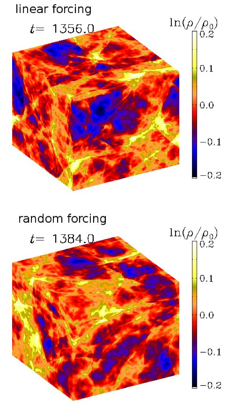
Figure 6: (online colour at: www.an-journal.org) Visualization of the logarithmic density (proportional to logarithmic pressure fluctuations) on the periphery of the domain for linear and random forcings. In both cases we have $\mbox{\rm Re}\approx 600$ at a resolution of $512^{3}$ mesh points.

In Table 1 we summarize integral and dissipation wavenumbers as well as the normalized energy fluxes for both linear and monochromatic random forcings. In wind tunnel turbulence one usually expresses the energy flux in units of a quantity $C_{\epsilon}=u^{\prime 3}/L$, where $u^{\prime}=u_{\rm rms}/\sqrt{3}$ is the one-dimensional rms velocity and $L=3\pi/4k_{\rm f}$ is the customary definition of the integral scale. The standard result of $C_{\epsilon}\approx 0.5$ ([Pearson et al. 2004]) corresponds then to $\epsilon\approx 0.04k_{\rm f}u_{\rm rms}^{3}$. Comparing the normalized energy fluxes for linear and monochromatic random forcings we see hardly any differences. This suggests that the nature of the forcing in hydrodynamic turbulence might not be of great qualitative importance, although it is still possible that the bottleneck effect ([Falkovich 1994]; [Dobler et al. 2003]) near the dissipative scale might be connected with the nature of the forcing at large scales ([Davidson 2004]).

Table 1: Summary of the normalized characteristic wavenumbers $\tilde{k}_{\rm f}=k_{\rm f}/k_{1}$, $\tilde{k}_{\rm d}=k_{\rm d}/k_{1}$, $k_{\rm Tay}=k_{\rm Tay}/k_{1}$, and $\tilde{k}_{\rm eff}=k_{\rm eff}/k_{1}$, for linear and monochromatic forcings. The numerical resolution is given in the second column.

linear forcing monochromatic forcing Re Res. $\tilde{k}_{\rm f}$ $\tilde{k}_{\rm d}$ $\tilde{k}_{\rm Tay}$ $\tilde{k}_{\rm eff}$ $\epsilon/k_{\rm f}u_{\rm rms}^{3}$ $\tilde{k}_{\rm f}$ $\tilde{k}_{\rm d}$ $\tilde{k}_{\rm Tay}$ $\tilde{k}_{\rm eff}$ $\epsilon/k_{\rm f}u_{\rm rms}^{3}$ 40 $64^{3}$ 1.6 15 3 3 0.080 1.6 12 2 3 0.072 70 $128^{3}$ 1.9 23 4 5 0.069 1.9 20 3 4 0.052 130 $128^{3}$ 2.0 40 6 6 0.073 1.9 34 4 7 0.045 300 $256^{3}$ 2.2 79 9 7 0.067 2.8 68 7 8 0.028 600 $512^{3}$ 2.2 133 13 10 0.069 1.2 130 8 3 0.064

In Table 1 we also list the values of $k_{\rm Tay}$ and $k_{\rm eff}$, as defined in Eqs (3) and (5). Both wavenumbers are clearly proportional to $\mbox{\rm Re}^{1/2}$, as can be seen from Fig. 7, where we plot the Reynolds number dependence of the ratios $k_{\rm Tay}/k_{1}$ and $k_{\rm eff}/k_{1}$ for linear and monochromatic forcings.

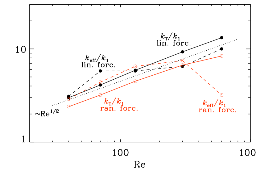
Figure 7: (online colour at: www.an-journal.org) Scalings of $k_{\rm Tay}/k_{1}$ (solid lines) and $k_{\rm eff}/k_{1}$ (dashed lines) with Re for linear (filled symbols) and monochromatic (open symbols and red lines) forcings. The dotted line indicates $\mbox{\rm Re}^{1/2}$ scaling.

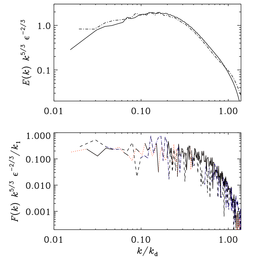
Figure 8: Comparison of compensated kinetic energy and helicity spectra for the linear forcing model (solid line) and the monochromatic random forcing function (dashed). In those patches where the kinetic helicity is negative, the modulus of the value is plotted as a dotted line (red for the linear forcing model and blue for the monochromatic random forcing function).

To compare the linearly and monochromatically forced turbulence simulations in real space, we present in Fig. 6 visualizations of the logarithmic density on the periphery of the computational domain. The logarithmic density is a convenient scalar quantity characterizing the pressure fluctuations resulting from the Reynolds stress. These visualizations look rather similar in the two cases, suggesting that the slight difference seen in the power spectra in Figs. 1 and 4 is hard to discern in such images. In fact, upon closer comparison of just the cases with the highest resolution we see that both kinetic energy and kinetic helicity spectra agree almost perfectly (Fig. 8), except that in the linear forcing model the kinetic energy spectrum has dropped significantly at the smallest wavenumber, which is not the case for monochromatic random forcing.

4 Conclusions

The linear forcing model is based on the driving of turbulence by a linear instability instead of a forcing function that is independent of the flow. This type of forcing might be more physical, because it does not change abruptly and depends on the local flow properties. Nevertheless, both types of forcing are Galilean invariant. This would change if the flow-independent monochromatic forcing were no longer $\delta$ correlated in time. A disadvantage of linearly forced turbulence is that energy injection occurs at all wavenumbers. Our simulations show that the energy spectrum is perhaps slightly shallower than with the flow-independent monochromatic forcing function. Part of this is explained by the bottleneck effect ([Falkovich 1994]; [Dobler et al. 2003]), and that the energy spectra compensated by $k^{5/3}$ show a stronger uprise toward the dissipation wavenumber. It is unclear whether this result would persist at larger resolution.

The linear forcing model has the interesting property of amplifying not only kinetic energy, but also kinetic helicity. Indeed, at early times, just after having injected kinetic helicity into the system, the coherent helical part continues to increase exponentially, but the flow soon breaks up into smaller eddies, giving rise to enhanced effective dissipation. For practical applications, it should be noted that the linear forcing model has the disadvantage that the initial exponential growth of kinetic energy and kinetic helicity might prevail for too long. This will be the case when the initial random perturbations are too weak to perturb the flow sufficiently. In that case, the kinetic energy would quickly increase to large values without producing three-dimensional turbulence.

With regards to geophysical and astrophysical applications we can say that in a turbulent system, kinetic helicity is no longer a conserved quantity, even though it would be if $\nu=0$ were strictly true. The latter requirement is of course not really possible in a turbulent system, because kinetic energy would then accumulate at the smallest possible scale resolved within the hydrodynamics framework and kinetic energy would not be able to decay, which is unphysical. While this should not be surprising, it is important to remember that this is quite different in the case of magnetohydrodynamics, where magnetic helicity dissipation really does go to zero in a turbulent system – even for finite (but small) values of the magnetic diffusivity. At the same time, magnetic energy dissipation does stay finite and is able to accomplish magnetic reconnection on the smallest resolved scales of the turbulent cascade ([Galsgaard & Nordlund 1996]; [Lazarian & Vishniac 1999]).

This paper has also shown that, regardless of the nature of the forcing, there are fairly strong helicity fluctuations. They appear to be coherent over many turbulent eddy timescales. One may wonder how generic such fluctuations are and if such fluctuations could be relevant for say the incoherent dynamo effects that have been investigated by several authors in recent years ([Vishniac & Brandenburg 1997]; [Sur & Subramanian 2009]; [Heinemann et al. 2011]; [Mitra & Brandenburg 2012]; [Richardson & Proctor 2010]). It will therefore be interesting the associate the kinetic helicity fluctuations with those of $\alpha$, which have already been determined in simulations of turbulent shear flows ([Brandenburg et al. 2008]).