Rational Term Structure Models with
Geometric Lévy Martingales
Abstract
In the “positive interest” models of Flesaker-Hughston, the nominal discount bond system is determined by a one-parameter family of positive martingales. In the present paper we extend this analysis to include a variety of distributions for the martingale family, parameterised by a function that determines the behaviour of the market risk premium. These distributions include jump and diffusion characteristics that generate various properties for discount bond returns. For example, one can generate skewness and excess kurtosis in the bond returns by choosing the martingale family to be given by (a) exponential gamma processes, or (b) exponential variance gamma processes. The models are “rational” in the sense that the discount bond price is given by a ratio of weighted sums of positive martingales. Our findings lead to semi-analytical formulae for the prices of options on discount bonds. A number of general results concerning Lévy interest rate models are presented as well.
I Interest rate models: the volatility approach
From a modern perspective there are two main approaches to the modelling of interest rates. These are the “volatility approach” and the “pricing kernel approach”. Both have been investigated extensively in the case of a Brownian filtration, but rather less so in the general situation when bond prices are allowed to jump. The main purpose of this paper is to present some new term structure models admitting, jumps based on parametric families of geometric Lévy martingales; but in doing so we shall take the opportunity to make some observations about the present state of interest rate modelling, both in the Brownian setting and the more general Lévy-Ito setting.
The volatility approach, in the case of a Brownian market filtration, is at present perhaps the most important and widely implemented interest rate modelling methodology, and it is the best understood. The celebrated HJM framework (Heath et al. 1992) belongs to this category, as does also the so-called Libor market model in its various manifestations (see e.g. Rebonato 2002, Musiela & Rutkowski 2005, and references cited therein), and a number of the “classical” short-rate models can be reformulated in this way as well. The volatility approach thus deserves special attention. We shall discuss the Brownian case first, and then its rather less well understood extension to the jump category.
The setup is as follows. The discount bond volatility, the market price of risk, and the initial yield curve, constitute the “primitive data” of the model. We have a probability space equipped with the augmented filtration associated with a Brownian motion of one or more dimensions. Here and in what follows denotes the “physical” measure; most of the discussion will focus on rather than on alternative measures. The interest rate markets are represented by a system of unit-principal discount bonds and a unit-initialised money-market account satisfying a system of dynamical equations of the following form:
| (1) |
Here is the random value at time of the bond that matures at time , is the short rate, is the bond volatility, and is the market price of risk. In the multi-dimensional setting, , , and are vector-valued processes, and in equation (1) there is an implied “dot product” between and , and also between and . We shall assume that the family of processes is differentiable with respect to in a suitable sense. We also assume that the family of processes is differentiable with respect to in a suitable sense, and that for any fixed it holds that . For some versions of the theory (such as the original formulation of HJM) one imposes a finite time horizon over which the model is defined; whereas for other versions the time horizon is infinite. We mostly consider the latter case here, and we assume that .
Given the initial bond prices , we find, under suitable conditions, that the solution for the discount bond system is
| (2) |
and that for the money-market account we have
| (3) |
We require, in particular, that the conditions
| (4) |
hold almost surely for all . If we set for all , we can invert equation (2) to obtain
| (5) |
For the short rate we then have
| (6) |
where denotes differentiation with respect to . Putting these ingredients together we are led to the following expression for the bond prices:
| (7) |
Here denotes the -forward price made at time for a -maturity bond. We see that and are determined by the specification of the volatility , the market price of risk , and the initial bond prices . This is the sense in which these are the primitive data of the model. In particular, there is no need to model the short rate as such separately—it is a “derived” quantity in the volatility approach. Two further conditions are required, namely, that the processes and defined by
| (8) |
for , and
| (9) |
for , are martingales (rather than merely local martingales). These conditions are needed if we are to make economic sense of the models and to put them into practice.
But how do we put the volatility approach into practice? As long as we are primarily interested in pricing and hedging, but less so (at least from a modelling perspective) in portfolio allocation, scenario analysis, and forecasting, then a transformation to the risk-neutral measure has the effect of removing the market price of risk from the equations; and the problem of modelling the evolution of the term structure of interest rates is transformed into the problem of modelling under . In the methodology that has been adapted by practitioners the idea is that we specify exogenously, under or under an appropriate set of forward measures, up to some overall parametric or functional freedom. This freedom is used to calibrate the model to the prices of derivatives, typically interest rate caps and swaptions. The general line of attack outlined above has in one form or another been widely implemented by financial institutions, and has been in use for more than two decades.
The volatility approach does nevertheless suffer from various defects, conceptual and practical, and it is reasonable to ask if one can do better. We shall not attempt a detailed critique here, but the following points can be made. One problem with the volatility approach is that it is difficult to impose a transparent condition on the discount bond volatility structure that ensures interest rate positivity (see, e.g., Brody & Hughston 2002). There is no clear economic motivation for choosing one volatility structure over another, and the fact that the volatility is modelled in the risk-neutral measure (or some other “unnatural” measure) further removes the model from economic reality. In this respect the elimination of the market price of risk is ultimately a shortcoming rather than a virtue. Originally it was thought that (following the triumph of the Black-Scholes formula) the lack of any need to model the actual returns of bonds was a “good thing”. The argument was that market volatilities could be inferred from option prices, whereas market returns could not, and therefore it would save a lot of trouble if one could avoid having to model the latter. But those were the days in which “derivative risk management” was mostly about pricing and hedging. The industry is wiser now, and there is a general perception to the effect that “buy side” concerns, which have always been somewhat less well-developed mathematically, involving the aforementioned issues of portfolio allocation, scenario analysis, and forecasting, are just as relevant to the “sell side” as they are to their colleagues on the other side of the Chinese wall. This argues for the reinstatement of and the abolition of .
II Pricing kernel approach
An alternative to the volatility approach is to base the theory on pricing kernels. The pricing kernel method allows for interest rate positivity, and it generalises readily to models not based on Brownian motion. The connection with economic thinking is clearer, and the extension to other asset classes (such as foreign exchange or inflation-linked products) is cleaner. The method is rooted in , so that although the use of other measures arises naturally enough in the course of various specific calculations there is no temptation to model “in the risk neutral measure” from the outset, a short cut that has often been taken in industry implementations in the past, but is in the final analysis limiting. It follows also that is present all along in the pricing kernel approach as part of the modelling framework, and is not swept underneath a -rug.
The idea is as follows. We assume the absence of arbitrage opportunities, but not market completeness. The filtration , which we take to satisfy the “usual conditions”, need not be Brownian, so jumps can be accommodated. Asset price processes have the càdlàg property. We assume the existence of an established pricing kernel satisfying almost surely for , and such that for any asset with price process and cumulative dividend process , the associated “deflated” or “discounted, risk-adjusted” price process defined by
| (10) |
is a -martingale. Thus if represents the price of an asset that pays no dividend, then is a martingale. If an asset delivers a single random cash flow at , and derives its value from that cash flow, then its value at is
| (11) |
In the case of a discount bond, which generates a cash flow of unity at , we have
| (12) |
for . It follows that we can use the pricing kernel as a basis for interest rate modelling. In particular, if we model parametrically, then we can generate families of bond price processes, and use the resulting freedom to calibrate the model to the prices of select market instruments, as in the volatility approach.
According to Ushbayev (2011), the notion of a “pricing kernel” dates back to the 1970s, and is used for example in Ross (1978), who has apparently modified the term “market kernel” used by Garman (1976). Authors have employed a variety of terms for essentially the same concept. Economists often speak of the “marginal rate of substitution”. The term “state price density” appears in Dothan & Williams (1978). One finds the term “stochastic discount factor” in Cox & Martin (1983), whereas the term “state price deflator” is used by Duffie (1992).
The idea of using the pricing kernel as a basis for interest rate modelling appears rather explicitly in Constantinides (1992). The following brief excerpt from this reference is indicative of the point of view proposed therein (we have changed his notation slightly to conform with ours): “We assert the existence of a positive state-price density or pricing kernel such that the nominal price at time of a claim to a nominal payoff at some future date is given by [our equation] (12), where denotes the expectation conditional on the information at time . The approach taken here is to explore directly the time-series process of , which yields plausible implications about the term structure of interest rates. I stress that in this approach it is unnecessary to assume a representative consumer economy in which the consumer has von Neumann-Morgenstern preferences.”
There are several different but more or less equivalent ways of representing the structure of the pricing kernel. Perhaps the most straightforward is to regard the short rate and the market price of risk as being the primitive data, and write the pricing kernel in the form
| (13) |
This line of attack works particularly well in the case of the “classical” short rate models, such as those of Vasicek (1977) and Cox et al. (1985), where one typically starts with an ansatz for the interest rate and the market price of risk. Then one can deduce the bond prices by use of (12), and the prices of derivatives based on bond prices (i.e. interest rate derivatives) by use of (11). The difficulty of this approach is that from an economic perspective it is unnatural to model the interest rate and market risk aversion processes “separately”. In economic analysis, these typically go hand in hand. Furthermore, the initial term structure is buried away in the specification of the primitive date, and there is no obvious prescription for calibrating the model, so one has to proceed on a case by case basis. Indeed, this is just what practitioners did before the advent of the HJM method.
We are thus led to ask the following question: do we actually lose anything by adopting the pricing kernel method, as opposed to the volatility method? In a Brownian setting the answer is no. In fact, the pricing kernel itself can be expressed in terms of the volatility , the market price of risk , and the initial bond prices , as follows:
| (14) |
This can be proved if, making use of (3), one inserts (5) into (13) and simplifies the result (see Jin & Glasserman 2001 and Tsujimoto 2010). Thus, any Brownian “volatility model” can be converted into a “pricing kernel model” and vice-versa. More precisely, we can regard , , and as being specified up to some overall parametric freedom, thus inducing a corresponding parametrisation of the pricing kernel, which can then be calibrated to market data and/or market forecasts by various schemes.
The upshot of this is that the various “approaches” to modelling interest rates amount to different ways of representing the pricing kernel, such as the formulae given by (13) and (14), which in turn suggest various distinct way of parameterising the resulting models. We shall, in what follows, consider yet another representation of the pricing kernel, namely that associated with the so-called Flesaker-Hughston (FH) models. In this representation (Flesaker & Hughston 1996, 1997, 1998) the pricing kernel takes the form
| (15) |
where is a family of positive unit-initialised martingales. Thus, we require that for , that for , and that for . It follows from the assumed asymptotic property of the initial term structure, without further restriction on the martingale family, that the right side of (15) is finite almost surely. In particular, by use of the Fubini theorem, the martingale property, and the fundamental theorem of calculus, one finds that . As a consequence of equation (12) we deduce that the discount bond system takes the rational form
| (16) |
To model the interest rate system we thus need to specify the initial term structure together with a family of positive martingales. The FH model originated as an attempt to characterise the complete family of HJM-type models with positive interest rates and valid over an arbitrary time horizon. The work was presented at the Cornell/Queen’s University Derivative Securities conference organised by R. Jarrow and S. Turnbull in April 1995 (cf. Hughston 2003). A generalised version of the model was presented by Rutkowski (1997), and it was made clear in this later work that the model was not tied to the use of a Brownian filtration. In the words of Rutkowski (1997): “From a theoretical viewpoint, the basic input of the generalised Flesaker-Hughston model is a strictly positive supermartingale …”. The relation of the FH models to the HJM theory and other approaches has been discussed in detail by a number of authors, including Jin & Glasserman (2001), Cairns (2004), Hunt & Kennedy (2004), Musiela & Rutkowski (2005), and Bjork (2009). Other representations of the pricing kernel method that offer interesting insights include the use of potentials (Rogers 1997), and Wiener chaos (Brody & Hughston 2004, Hughston & Rafailidis 2005); these will not be considered here. We return to the FH representation in the context of Lévy models.
III Lévy models for interest rates
One important deficiency of the volatility approach to interest rate modelling is that in its more successful implementations it has been so deeply intertwined with Brownian motion based modelling techniques that little by way of consensus has emerged either in the industry or among academics on how best to incorporate jumps into the scheme. This being the case, it will not be amiss here to attempt to make some progress on the matter.
The theory of Lévy models for asset pricing has an extensive literature. We refer the reader, for example, to Madan & Senata (1990), Madan & Milne (1991), Heston (1993), Gerber & Shiu (1994), Eberlein & Keller (1995), Eberlein & Jacod (1997), Chan (1999), Kallsen & Shiryaev (2002), Fujiwara & Miyahara (2003), Schoutens (2003), Cont & Tankov (2004), Esche & Schweizer (2005), Hubalek & Sgarra (2006), and references cited therein. By a Lévy process on a probability space we mean a process such that , is independent of for , and for . Here denotes the augmented filtration generated by . For to give rise to a Lévy model for asset prices, we require that it should possess exponential moments; that is,
| (17) |
for , for in some connected real interval containing the origin. The stationary and independent increments property implies that there exists a Lévy exponent such that
| (18) |
for . Then the process defined by
| (19) |
is a martingale, called the associated geometric Lévy martingale (or Esscher martingale), with parameter . More generally, let be an –predictable process, chosen in such a way that for , and such that the local martingale defined by
| (20) |
is a martingale. If a predictable process satisfies these conditions then we say it is admissible. Then we are led to consider an asset pricing model of the following form. Let the exogenously specified short rate be –adapted, and be such that the unit-initialised money market account defined as in (3) is finite almost surely for . Let the -adapted risk aversion and volatility processes and be positive, and be such that , , and are admissible in the sense noted above. The pricing kernel is taken to be given by
| (21) |
and the associated expression for the price of a typical non-dividend-paying asset is
| (22) |
where
| (23) |
is the excess rate of return function associated with the given Lévy exponent. It is a remarkable property of the function , arising as a consequence of the convexity of the Lévy exponent, that if the volatility and the risk aversion are positive, then the excess rate of return is positive, and is monotonically increasing in its arguments (Brody et al. 2011). In general the excess rate of return is nonlinear, and hence in a general Lévy setting the process no longer admits the interpretation of being the market price of risk, but instead should be viewed as a measure of investor risk aversion.
The theory of interest rates can be developed in just this spirit in a way that generalises the HJM framework to the Lévy category. In particular, we are able to give a consistent treatment of the risk premium associated with interest rate products in such a way that the risk premium is positive for bonds. Interest rate models admitting jumps have been pursued by a number of authors, including, inter alia, Shirakawa (1991), Jarrow & Madan (1995), Björk et al. (1997), Björk et al. (1997), Eberlien & Raible (1999), Raible (2000), Eberlein et al. (2005), Eberlein & Kluge (2006a,b, 2007), and Filipović et al. (2010), to mention a few. Our approach is novel inasmuch as we introduce a pricing kernel at the outset, rather than attempting to model the interest rate system through a set of dynamical equations. A rather general class of Lévy interest rate models exhibiting the positive excess rate of return property can thus be constructed as follows. The idea is to model the pricing kernel and the associated discount bond system. There is no need to introduce a system of instantaneous forward rates. Let the pricing kernel be given by (21), and write for the price at of a bond that matures at to deliver one unit of currency. For the Lévy discount bond model we have:
| (24) |
We require (a) that and are positive, (b) that , , and , are admissible in the sense indicated above, and (c) that should vanish as approaches . The maturity condition allows one to solve for the money market account in terms of and , as in the Brownian case:
| (25) |
Inserting the expression for the money market account back into the bond price, we obtain:
| (26) |
where . If we substitute the expression for the money market account back into equation (21), and simplify the result, we deduce the following:
Proposition 1.
The pricing kernel in a Lévy interest rate model can be expressed in terms of the initial term structure , the bond volatility , and the risk aversion as:
| (27) |
This result offers one a rather general method for modelling an arbitrage-free interest rate system in the physical measure when there are jumps. In particular, if we model the volatility structure and the risk aversion exogenously, and specify the initial term structure, then we determine the pricing kernel, the discount bond system, and the money market account. In practice, as in the Brownian case, the volatility structure and the risk aversion process can be modelled parametrically, up to some undetermined functional degrees of freedom, to be fixed by calibration to the prices of market instruments at time zero. Indeed, one could treat the Lévy exponent itself as part of the “functional freedom” of the model.
One can also consider an extension of the FH models to the Lévy category as a basis for representing the pricing kernel. We shall construct the required martingale families from the Esscher martingales associated with various Lévy processes. Thus we fix a probability space and a Lévy process admitting exponential moments as before, and for a suitable deterministic function we define a martingale family by setting
| (28) |
We note that and . We require that for all . By making various choices for we are thus able to generate a variety of interest rate models, each with some functional freedom given by the choice of . In the general setting, both and are vectorial, and the components of are independent processes. For the present we look at one-dimensional models. In Section IV we consider first the case of a geometric Brownian motion (GBM) family. In this instance there are of course no jumps, but the calculations involved are indicative of the more general case, and are of some interest in their own right. Expressions are derived for discount bonds, the short rate, the bond volatility, and the risk aversion. In Section V we establish necessary and sufficient conditions on to ensure the positivity of the risk premium in the case of the GBM family, and in Section VI we solve the associated option pricing problem. In Sections VII, VIII, and IX we proceed to construct models based on the Esscher martingale families associated with jump-diffusion processes, gamma processes, and variance-gamma processes, and to examine their properties.
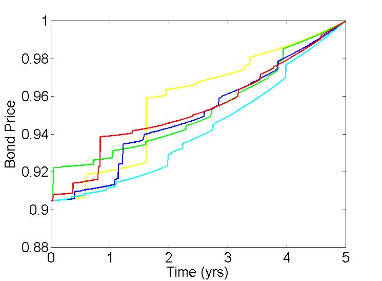
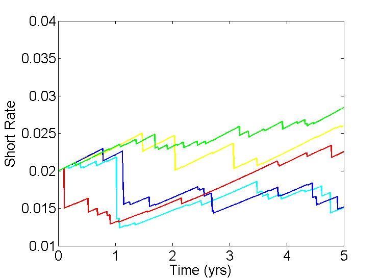
IV GBM family
Writing for a standard Brownian motion, we obtain a geometric Lévy martingale family of the form
| (29) |
for . This leads to the following system of discount bond prices:
| (30) |
for (cf. Brody & Friedman 2009). The function denotes the initial “term-structure density” (Brody & Hughston 2001), and is given by We make note of the fact that if the initial interest rates are positive and if , then fulfils the requirements of a density function: namely, that for , and that
| (31) |
By use of the relation it follows that the short rate is of the form
| (32) |
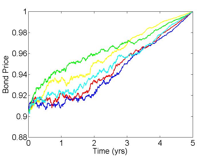
Simulations of the bond price (30) and the short rate (32) are presented in Figure 1. We note that need not in general be bounded from above. Some rational term-structure models, such as the rational lognormal model (Flesaker & Hughston 1996), and the separable second-chaos models (Hughston & Rafailidis 2005) have bounded interest rates. See Cairns (2004) for further discussion on this point.
By an application of Ito’s lemma to equation (30), we deduce that the dynamical equation of the bond price system is given by
| (33) |
where
| (34) |
and . We note that the bond volatility is of the form and that the market price of risk is given by The bond volatility and the market price of risk together give us the risk premium associated with an investment in a discount bond:
| (35) |
Since and are determined by , which in turn is determined by and via (34), we conclude that the model is fully characterised by the specification of the initial term structure and the martingale volatility structure . It is worth remarking that even if the volatility of the martingale family (29) is deterministic, both the bond price and the short rate exhibit nontrivial stochastic dynamics.
V Positivity of risk premium in the GBM family
In the case of a volatility-based representation for the pricing kernel we were able to identity the condition for the positivity of the excess rate of return above the short rate. That is, we require that , where is defined by (23), and this can be satisfied if we specify exogenously that the risk aversion and the volatility are positive. In the case of an FH model, it is not immediately apparent from expression (35) for the excess rate of return that the required conditions are satisfied. Since is fixed by the initial term structure, the relevant condition for the positivity of the excess rate of return must be imposed on the choice of the functional model parameter . We shall establish necessary and sufficient conditions on such that .
Proposition 2.
In an FH model based on a GBM family with functional model parameter , a sufficient condition to ensure that the risk premium is positive is that either should be positive and decreasing, or that should be negative and increasing.
Proof. Suppose that is positive for all . Then it follows from (34) that is positive. Differentiating (34) with respect to we obtain
| (36) |
where
| (37) |
is the instantaneous forward rate defined as usual by which is positive in any FH model. Next we observe that (34) can be written in the form
| (38) |
where
| (39) |
Note that is positive and that
| (40) |
Thus, according to (38), is a weighted average of the values of for greater than or equal to . It follows that if is decreasing as a function of , then , for . This in turn implies, by use of (36), that , and hence by (35) that the risk premium is positive. A similar argument shows that if is negative and increasing for , then the risk premium is positive.
Proposition 3.
In an FH model based on a GBM family with functional model parameter , assume that for any admissible initial term-structure density the risk premium is positive. Then must be either positive and decreasing, or negative and increasing.
Proof. If , then either (i) and holds; or (ii) and holds. Assume that (ii) holds. Let us define a random probability measure by setting where is defined in (39). Note that has the property that . We can then express the condition in the form
| (41) |
which must hold for all . Specifically, at we have
| (42) |
Since this has to hold for an arbitrary density , it has to hold, in particular, for the limiting case of a delta function for any . It follows that must be negative for all . Next we observe that since holds by assumption, the fact that this inequality must hold, in particular, for slightly greater than implies that
| (43) |
for all . By (36) and the fact that the instantaneous forward rates are positive, we deduce that for all . Therefore, we obtain
| (44) |
for all . Now letting for any , we deduce that . Similar arguments can be used in the case where (i) and holds.
VI Option Pricing in the GBM case
We consider the option pricing problem in the case of the geometric Brownian motion family. First we discuss the problem of option pricing in a general Lévy model, and then we specialise to the Brownian case. The price at time of a European call option expiring at time , with strike price , on a discount bond maturing at time , is given by
| (45) |
We assume that . By use of (12) it follows that
| (46) |
and hence by (16) we have
| (47) |
Recall that the martingale family appearing in (47) takes the form
| (48) |
For an option price in the general setting we thus obtain
| (49) |
We observe that if is decreasing in , then the function defined by
| (50) |
is decreasing in the variable . The argument is as follows. A short calculation shows that
| (51) |
where the function is defined by
| (52) |
We observe that if is decreasing then
| (53) |
This follows from the fact that
| (54) |
where
| (55) |
We note that is for each value of a weighted average of for . Thus, if is decreasing, then the right-hand side of equation (54) is negative. If the right-hand side of (54) is positive (resp. negative) then (51) is positive (resp. negative). It follows that if is decreasing in , then is decreasing in , as claimed. A similar argument shows that if is increasing in for all then is increasing in .
Let us assume now that is monotonic in , and write and for the upper and lower extremal values of as varies. Then for any in the range we can find a number such that
| (56) |
This enables us to truncate the expectation in (49) at the point where the maximum function becomes nonpositive. The price of an option in the general Lévy case then takes the form
| (57) |
where
| (58) |
and is the Heaviside function. In particular, when the underlying Lévy martingale is a geometric Brownian motion, and is positive and decreasing, the option price simplifies to the following expression:
| (59) |
where denotes the normal distribution function. We remark that when is a strictly monotonic function the resulting discount bond prices and interest rates are Markovian. This is because the functions and are monotonic functions of , and and .
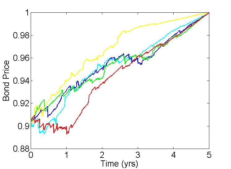
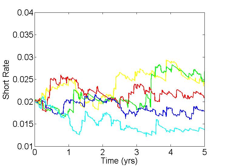
VII Geometric jump-diffusion family
Merton (1976) extended the Black-Scholes option-pricing theory to include equity prices driven by a jump-diffusion process. In term-structure modelling it is also desirable to incorporate both jump risk and diffusion risk. For simplicity we focus on the case of normally distributed jump sizes. We introduce a Poisson process , with rate parameter , to represent the number of jumps occurring by time . The size of the jump is modelled by a random variable . Jump sizes are independent and identically distributed random variables, each such that . If the diffusion component is driven by an independent Brownian motion , we obtain an expression for the bond price as follows. Writing for the compound Poisson process defined by
| (60) |
and introducing a single functional degree of freedom , by use of (28) we obtain a geometric martingale family of the form
| (61) |
This leads to the following discount bond price:
| (62) |
and for the short rate we have
| (63) |
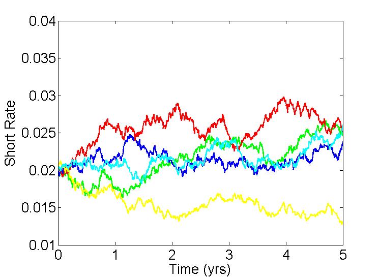
Sample paths of the bond price (62) and the short rate (63) are simulated in Figure 2. In Merton (1976) a key idea used to price options is the notion that idiosyncratic risk can be modelled with a return equal to the risk-free rate. In Merton’s model it is assumed that the jump risk is purely idiosyncratic and can be diversified away by holding a suitably broad portfolio. In our model jump risk is being priced. The resulting risk premium is implicit in the choice of pricing kernel, and is determined by the functional model parameter .
To derive an expression for the price of a call option with strike , we need to evaluate the expectation in (49). By use of the tower property of conditional expectation we condition on the number of Poisson jumps to obtain
| (64) |
Our task is first to compute the conditional expectation, which is essentially Gaussian, and then the unconditional expectation, which is an expectation over the Poisson randomness. As we have shown in the previous section, if is decreasing for then we can find a number such that , where
| (65) |
Hence, after a calculation, we are able to deduce that the price of a call option in the case of a geometric jump-diffusion martingale family is given by
| (66) | |||||
where and .
VIII Geometric Gamma Family
We begin with a brief review of the theory of the gamma processes. Let and be positive constants. By a gamma process with growth rate and variance rate we mean a process with independent increments such that and such that has a gamma distribution with mean and variance . Writing and , we have and . The density of is then given by
| (67) |
for . Here is the standard gamma function, which for is defined by
| (68) |
A calculation shows that for the moment generating function of is given by
| (69) |
from which it follows that and . The exponential martingale associated with is given by . See Schoutens (2003), Cont & Tankov (2004), Yor (2007), and Brody et al. (2008) for further details of the gamma process.
Now fix and , let the function satisfy for , and define a one-parameter family of positive martingales by setting
| (70) |
Writing { as before for the initial term structure density, we obtain from equation (16) the following expression for the discount bond prices:
| (71) |
and for the associated short rate we have
| (72) |
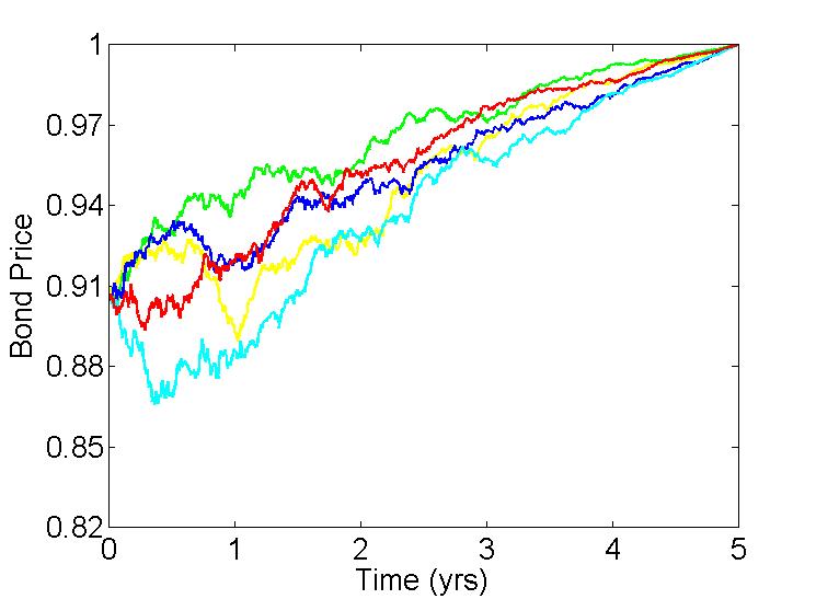
Sample paths associated with the bond price and the short rate are shown in Figure 3. Since a gamma process only has upward jumps, and since the bond price is an increasing function of the underlying Lévy process when is (negative and) increasing, we find that jumps in induce downward jumps in the short rate process, as is evident from the simulation.
In the geometric gamma model we can obtain a semi-analytical expression for the price of a European style call option with strike price . As in previous sections we know that if is negative and increasing for then we can find a such that , where in this case we define
| (73) |
We deduce, using (49), that the price of the call option is given by
| (74) |
Here we have written
| (75) |
for the upper incomplete gamma function.
IX Geometric VG Family
A more sophisticated model can be constructed if the underlying Lévy process is taken to be of the variance gamma (VG) type. The VG process was introduced in the finance literature by Madan & Seneta (1990), and since then has been studied by a number of authors (see, e.g., Madan et al. 1998). It will be useful for our purposes to begin with a brief exposition of the theory of the VG process, treating it in a manner consistent with our earlier discussion of the gamma process. Let and be a pair of independent gamma processes, each with scale parameter unity and rate parameter . Thus and , and similarly for . Now let , be a pair of nonnegative constants and set
| (76) |
To investigate the properties of the process thus defined we calculate the moment generating function of . The result is:
| (77) |
for in a suitable range. We claim that is identical in law to a process of the form
| (78) |
where and are constants, where is a scaled gamma process satisfying , and where represents the subordination of a standard Brownian motion by . We shall refer to as a drifted VG process. To see the relation between and we calculate the moment generating function of to obtain
| (79) |
Here is the scale parameter of and is the rate parameter of . We observe that (77) and (79) take the same form if . The two moment generating functions can then be identified if we set and . Next we impose the normalisation , which implies . This allows us to express and in terms of , , and . We find that and and hence
| (80) |
Since and are Lévy processes, the fact that the moment generating functions agree is sufficient to ensure that the processes are identical in law. The theory of the VG process thus outlined is consistent with that of Madan et al. (1998). The parametrisation that we have chosen is for our purposes more transparent. In particular, the limiting cases where or are incorporated. We define a family of positive martingales by setting
| (81) |
Then, using equation (16), we deduce that the bond price takes the form
| (82) |
and that the associated short rate is given by
| (83) |
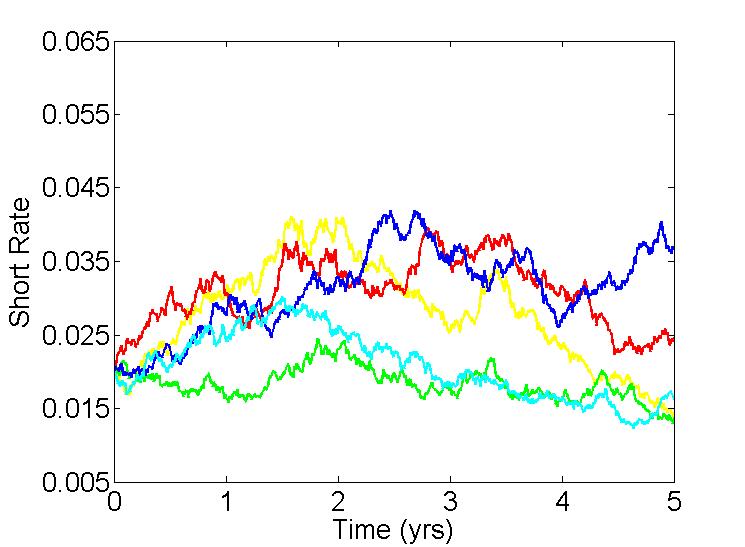
Simulations of the bond price (82) and the short rate (83) are presented in Figure 4.
We proceed to derive the price of a bond option in the setting of the geometric VG martingale family. In the case of a call option with expiry and strike on a bond with maturity , let us consider expression (47), into which we substitute (81). As before, when is decreasing for we are able to find a number such that , where
| (84) |
In terms of the critical level we deduce that the price of the option is given by
| (85) | |||||
where and
| (86) |
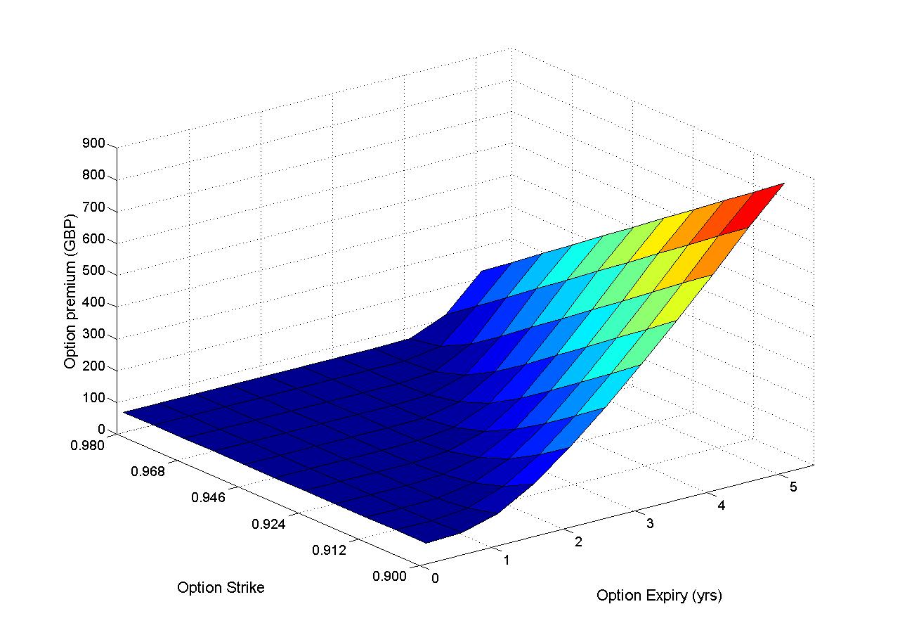
In Figure 5 we present examples of price surfaces of European-style call options for the jump-diffusion and VG families of models. The figures each contain one hundred prices computed over a range of strikes and option expiries. The computing times for one-hundred call prices for the Gaussian, jump-diffusion, gamma, and VG families of term-structure models were 6 seconds, 54 seconds, 10 seconds, and 6 seconds, respectively.

Acknowledgements.
The authors would like to thank seminar participants at the Imperial College Workshop on Stochastics, Control and Finance, London, April 2010, at the Fifth General Conference on Advanced Mathematical Methods in Finance, Bled, Slovenia, May 2010, at the Fields Institute Workshop on Financial Derivatives and Risk Management, Toronto, May 2010, at the Sixth World Congress of the Bachelier Finance Society, Toronto, June 2010, at the Workshop on Mathematical Finance and Related Issues, Kyoto, September 2010, at the Bank of Japan, Tokyo, September 2010, and at the Department of Economics, Hitotsubashi University, Tokyo, September 2010, for useful comments. L. P. Hughston thanks R. Miura, J. Sekine, and H. Sugita for hospitality. E. Mackie acknowledges support by EPSRC, and thanks A. S. Iqbal and S. Lyons for helpful discussions.References
- (1) Bjork, T. (2009) Arbitrage Theory in Continuous Time, third edition. Oxford University Press.
- (2) Bjork, T., Di Masi, G., Kabanov, Y., & Runggaldier, W. (1997) Towards a general theory of bond markets. Finance and Stochastics 1, 141-174.
- (3) Bjork, T., Kabanov, Y. & Runggaldier, W. (1997) Bond market structure in the presence of marked point processes. Mathematical Finance 7, 211-239.
- (4) Brody, D. C. & Freidman, R. (2009) Information of interest. Risk Magazine, December issue, 101-106.
- (5) Brody, D. C. & Hughston, L. P. (2001) Interest rates and information geometry. Proc. Roy. Soc. Lond. A 457, 1343–1364.
- (6) Brody, D. C. & Hughston, L. P. (2002) Entropy and information in the interest rate term structure. Quantitative Finance 2, 70–80.
- (7) Brody, D. C. & Hughston, L. P. (2004) Chaos and coherence: a new framework for interest rate modelling. Proc. Roy. Soc. Lond. A 460, 85-110.
- (8) Brody, D. C., Hughston, L. P. & Macrina, A. (2008) Dam rain and cumulative gain. Proc. Roy. Soc. Lond. A 464, 1801-1822.
- (9) Brody, D. C., Hughston, L. P. & Mackie, E. (2011) General theory of geometric Lévy models for dynamic asset pricing. arXiv:1111.2169.
- (10) Cairns, A. J. G. (2004) Interest Rate Models: An Introduction. Princeton University Press.
- (11) Chan, T. (1999) Pricing contingent claims on stocks driven by Lévy processes. Annals of Applied Probability 9, 504-528.
- (12) Constantinides, G. M. (1992) A theory of the nominal term structure of interest rates. Review of Financial Studies 5, 531-552.
- (13) Cont, R. & Tankov, P. (2004) Financial Modelling with Jump Processes. Chapman & Hall, London.
- (14) Cox, S. H. & Martin, J. D. (1983). Abandonment value and capital budgeting under uncertainty. J. Economics and Business 35, 331-341.
- (15) Cox, J. C., Ingersoll, J. & Ross, S. A. (1985) A theory of the term structure of interest rates. Econometrica 53, 385-407.
- (16) Dothan, U. & Williams, J. T. (1978). Valuation of assets on a Markov state space. Economics Letters 1, 163-166.
- (17) Duffie, D. (1992) Dynamic Asset Pricing. Princeton University Press.
- (18) Eberlein, E. & Jacod, J. (1997) On the range of option prices. Finance and Stochastics 1, 131-140.
- (19) Eberlein, E., Jacod, J. & Raible, S. (2005) Lévy term structure models: No-arbitrage and completeness. Finance and Stochastics 1, 67-88.
- (20) Eberlein, E. & Keller, U. (1995) Hyperbolic distributions in finance. Bernoulli 1, 281-299.
- (21) Eberlein, E. & Kluge, W. (2006a) Exact pricing formulae for caps and swaptions in a Lévy term structure model. J. Computational Finance 9, 99-125.
- (22) Eberlein, E. & Kluge, W. (2006b) Valuation of floating range notes in Lévy term structure models. Mathematical Finance 16, 237-254.
- (23) Eberlein, E. & Kluge, W. (2007) Calibration of Lévy term structure models. In: Advances in Mathematical Finance, Festschrift Volume in Honour of Dilip Madan. R. Elliott, M. Fu, R. Jarrow & Ju–Yi Yen (eds.). Birkhäuser, Basel.
- (24) Eberlein, E. & Raible, S. (1999) Term structure models driven by general Lévy processes. Mathematical Finance 9, 31-53.
- (25) Esche, F. & Schweizer, M. (2005) Minimal entropy preserves the Lévy property: how and why. Stoch. Proc. Appl. 115 (2), 299-327.
- (26) Filipović, D., Tappe, S. & Teichmann, J. (2010) Term structure models driven by Wiener process and Poisson measures: existence and positivity. SIAM J. Financial Mathematics 1, 523–554.
- (27) Flesaker, B. & Hughston, L. P. (1996) Positive interest. Risk Magazine 9, 46–49; reprinted in Vasicek and Beyond, L.P. Hughston (ed), Risk Publications, London (1996); and in Hedging with Trees: Advances in Pricing and Risk Managing Derivatives (M. Broadie & P. Glasserman, eds.), Risk Publications, London (1998).
- (28) Flesaker, B. & Hughston, L. P. (1997) International models for interest rates and foreign exchange. Net Exposure 3, 55–79; reprinted in The New Interest Rate Models, L. P. Hughston (ed.), Risk Publications, London (2000).
- (29) Flesaker, B. & Hughston, L. P. (1998) Positive interest: An afterword. In Hedging with Trees, M Broadie, P Glasserman (eds), London: Risk Publications.
- (30) Garman, M. B. (1976) A general theory of asset valuation under diffusion state processes. Working Paper No. 50, Institute of Business and Economic Research, U. California, Berkeley.
- (31) Gerber, H. U. & Shiu, E. S. W. (1994) Option pricing by Esscher transforms (with discussion). Transactions of the Society of Actuaries 46, 99-191.
- (32) Heath, D., Jarrow, R. & Morton, A. (1992) Bond pricing and the term structure of interest rates: a new methodology for contingent claims valuation. Econometrica 60, 77-105.
- (33) Heston, S. L. (1993) Invisible parameters in option prices. J. Finance 48, 993-947.
- (34) Hubalek, F. & Sgarra, C. (2006) On the Esscher transform and entropy for exponential Lévy models. Quantitative Finance 6, 125-145.
- (35) Hughston, L. P. (2003) The past, present, and future of term structure modelling. Chapter 7 in Modern Risk Management: A History, introduced by Peter Field, 107–132. Risk Publications, London.
- (36) Hughston, L. P. & Rafailidis, A. (2005) A chaotic approach to interest rate modelling. Finance and Stochastics 9, 43-65.
- (37) Hunt, P. J. & Kennedy, J. E. (2004) Financial Derivatives in Theory and Practice, revised edition. John Wiley Sons, Chichester.
- (38) Jarrow, R. & Madan, D. B. (1995) Option pricing using the term structure of interest rates to hedge systematic discontinuities in asset returns. Mathematical Finance 5, 311-336.
- (39) Jin, Y. & Glasserman, P. (2001) Equilibrium positive interest rates: a unified view. Review of Financial Studies 14, 187-214.
- (40) Kallsen, J. & Shiryaev, A. N. (2002) The cumulant process and Esscher’s change of measure. Finance and Stochastics 6 (4), 97-428.
- (41) Madan, D. Carr, P. & Chang, E. C. (1998) The variance gamma process and option pricing. European Finance Review 2, 79-105.
- (42) Madan, D. & Seneta, E. (1990) The variance gamma (V.G.) model for share market returns. J. Business 63, 511-524.
- (43) Madan, D. & Milne, F. (1991) Option pricing with V.G. martingale components. Mathematical Finance 1, 39-55.
- (44) Merton, R. C. (1976) Option pricing when underlying stock returns are discontinuous. J. Financial Economics 3, 125-144.
- (45) Musiela, M. & Rutkowski, M. (2005) Martingale Methods in Financial Modelling. Springer-Verlag, Berlin.
- (46) Raible, S. (2000) Lévy Processes in Finance: Theory, Numerics, and Empirical Facts, PhD Thesis, University of Freiburg.
- (47) Rogers, L. C. G. (1997) The potential approach to the term structure of interest rates and foreign exchange rates. Mathematical Finance 7, 157-176.
- (48) Ross, S. A. (1978) The current status of the capital asset pricing model (CAPM). J. Finance 33, 885-901.
- (49) Rutkowski, M. (1997) A note on the Flesaker-Hughston model of the term structure of interest rates. Applied Mathematical Finance 4, 151–163.
- (50) Schoutens, W. (2003) Lévy Processes in Finance: Pricing Financial Derivatives. Wiley, New York.
- (51) Shirakawa, H. (1991) Interest rate option pricing with Poisson-Gaussian forward rate curve processes. Mathematical Finance 1, 77-94.
- (52) Tsujimoto, T. (2010) Calibration of the chaotic interest rate model. PhD thesis, University of St Andrews.
- (53) Ushbayev, A. (2011) private communication.
- (54) Vasicek, O. (1977) An equilibrium characterisation of the term structure. J. Financial Economics 5, 177-188.
- (55) Yor, M. (2007) Some remarkable properties of gamma processes. In: Advances in Mathematical Finance, Festschrift Volume in Honour of Dilip Madan. R. Elliott, M. Fu, R. Jarrow & Ju–Yi Yen (eds.). Birkhäuser, Basel.