An investigation of the SCOZA for narrow square-well potentials and in the sticky limit

Abstract

We present a study of the self consistent Ornstein-Zernike approximation (SCOZA) for square-well (SW) potentials of narrow width $\delta$. The main purpose of this investigation is to elucidate whether in the limit $\delta\to 0$, the SCOZA predicts a finite value for the second virial coefficient at the critical temperature $B_{2}(T_{c})$, and whether this theory can lead to an improvement of the approximate Percus-Yevick solution of the sticky hard-sphere (SHS) model due to Baxter [R. J. Baxter, J. Chem. Phys. 49, 2770 (1968)]. For SW of non vanishing $\delta$, the difficulties due to the influence of the boundary condition at high density already encountered in an earlier investigation [E. Schöll-Paschinger, A. L. Benavides, and R. Castañeda-Priego, J. Chem. Phys. 123, 234513 (2005)] prevented us from obtaining reliable results for $\delta<0.1$. In the sticky limit this difficulty can be circumvented, but then the SCOZA fails to predict a liquid-vapor transition. The picture that emerges from this study is that for $\delta\to 0$, the SCOZA does not fulfill the expected prediction of a constant $B_{2}(T_{c})$ [M. G. Noro and D. Frenkel, J. Chem. Phys. 113, 2941 (2000)], and that for thermodynamic consistency to be usefully exploited in this regime, one should probably go beyond the Ornstein-Zernike ansatz.

I Introduction

Narrow attractive interactions are ubiquitous in the realm of colloidal dispersions. A most relevant instance is represented by depletion-induced forces in mixtures of highly asymmetric hard spheres, a field that has received a fundamental contribution by Bob Evans evans . Although these investigations have shown that the structure of effective depletion interactions is in general more complex than just a single attractive tail, a narrow attractive contribution at short distance is still to be expected in most cases, and its relevance to the modelization of both the equilibrium and non equilibrium phase behavior of colloidal systems has long been acknowledged.

In view of this, it is somewhat disappointing that the difficulties experienced by most liquid-state theories when phase separation occurs, the foremost of which is lack of convergence in a (not necessarily small) neighborhood of the critical region, only become worse when the range of the attractive potential decreases to a small fraction of the particle size. However, it may be argued that this is not a fundamental difficulty, inasmuch as this class of interactions can be dealt with by the sticky hard-sphere (SHS) model baxter . This is obtained from the prototypical attractive interaction, i.e., the hard-core plus square-well (SW) potential $v_{\rm SW}(r)$ given by

$$v_{\rm SW}(r)=\left\{\begin{array}[]{ll}+\infty\mbox{\hskip 28.45274pt}&r<\sigma\,,\\ -\epsilon&\sigma\leq r\leq(1+\delta)\sigma\,,\\ 0&r>(1+\delta)\sigma\,,\end{array}\right.$$ (1)

by taking the limits $\delta\to 0$, $\epsilon\to\infty$ so that the second virial coefficient $B_{2}$ stays finite and non vanishing:

$$\beta v_{\rm SHS}(r)=\left\{\begin{array}[]{ll}+\infty\mbox{\hskip 28.45274pt}&r<\sigma\,,\\ -\ln\left[\displaystyle{\frac{1}{12\tau}}(1+\displaystyle{\frac{1}{\delta}})\right]&\sigma\leq r\leq(1+\delta)\sigma\mbox{\hskip 28.45274pt}\delta\to 0\,,\\ 0&r>(1+\delta)\sigma\,.\end{array}\right.$$ (2)

The stickiness parameter $\tau$ is related to the second virial coefficient of the SHS model $B_{2}^{\rm SHS}$ by the relation

$$\tau=\frac{B_{2}^{\rm HS}}{4\,(B_{2}^{\rm HS}-B_{2}^{\rm SHS})}\,,$$ (3)

where $B_{2}^{\rm HS}=2\pi\sigma^{3}/3$ is the second virial coefficient of the hard-sphere fluid. As shown by Baxter baxter , this model be can solved exactly within the Percus-Yevick (PY) integral equation hansen . Because of the way the limit (2) is taken, the solution does not depend on the temperature, but rather on the stickiness $\tau$ or, equivalently, on $B_{2}^{\rm SHS}$. The connection between the SHS model and an actual fluid at a certain temperature $T$ can be made by a generalized principle of corresponding states that, although not rigorous, has been found to work remarkably well. According to this principle, usually referred to as Noro-Frenkel (NF) scaling noro , a pair potential $v(r)$ consisting of a hard-core repulsion with diameter $\sigma$ and an attractive tail $w(r)$ can be mapped into the SW potential (1), provided that the width $\delta$ of the attractive well is determined so that its second virial coefficient $B_{2}(T)$ will be the same as that of the original interaction at the same temperature $T$, assuming that in both cases $T$ is measured in units of the well depth. On the other hand, when $\delta$ is small, by following the same procedure the SW potential can in turn be mapped into the SHS model. In this way, NF scaling can be combined with Baxter analytical solution of the SHS model to provide a unified description of fluids with narrow attractive interactions. For instance, the critical temperature $T_{c}$ of such a fluid can be evaluated by that at which its $B_{2}(T)$ is equal to the critical value of $B_{2}^{\rm SHS}$.

Although the SHS model has a perfectly regular solution within the PY approximation and has also been the subject of intensive simulation studies seaton ; kranendonk ; miller ; miller2 , the singularity embedded into its very definition should instigate a mild feeling of suspicion. In fact, twenty-three years after the appearance of the model, Stell stell discovered that the latter from a rigorous statistical mechanical point of view is thermodynamically unstable whenever the number of particles is greater than eleven. However, the state of affairs is less serious than it might seem: the instability arises from a number of rather fancy particle configurations, that are readily destroyed by the slightest amount of polidispersity in the system. Therefore, the SHS model and its approximate analytical solution via the PY equation baxter still remain a valuable tool for the interpretation of the phase diagram of colloidal dispersions subject to short-range interactions.

There is, however, a significant limitation of this solution that negatively affects its predictive power, i.e., its lack of thermodynamic consistency. This is particularly evident when the liquid-vapor transition of the model is considered: the coexistence curves determined by the compressibility and internal energy routes described in Sec. II differ markedly from each other, the discrepancy between the critical densities amounting to nearly a factor three, and neither of them agrees quantitatively with the simulation results miller . In this respect, it is also worth recalling that the PY approximation upon which the analytical solution of the SHS is based, is expected to become less and less accurate as the density is increased, while on the other hand the critical density increases as the range of the interaction decreases, and for $\delta\to 0$ the limiting value predicted by the simulations miller ; largo is considerably larger than that expected for Lennard-Jones like fluids.

Recently, a different approach has emerged, which is based upon enforcing consistency between the aforementioned energy and compressibility routes to the thermodynamics, namely, the self-consistent Ornstein-Zernike approximation (SCOZA) scozayuk1 ; scozayuk2 ; scozayuk4 ; foffi ; scozaorea . This has been applied especially to the case in which $v(r)$ consists of a hard core and a Yukawa (HCY) attractive tail:

$$v_{\rm HCY}(r)=\left\{\begin{array}[]{ll}+\infty\mbox{\hskip 28.45274pt}&r<\sigma\,,\\ -\epsilon\,\displaystyle{\frac{\sigma}{r}}\,e^{-z(r/\sigma-1)}&r>\sigma\,,\end{array}\right.$$ (4)

where $z$ is the inverse-range parameter of the interaction. For the HCY potential, the SCOZA has shown a remarkable robustness even for very short-range tails, while still remaining accurate foffi ; scozaorea . On the other hand, one might argue that accuracy cannot be expected to persist for attractions of arbitrarily short range, since after all, as recalled in Sec. II, the SCOZA assumes that the direct correlation function $c(r)$ of the fluid is linear in the attractive part $w(r)$ of the interaction, and its low-density expansion does not even give back the correct expression of $B_{2}(T)$. In orpanl it was suggested that for narrow attractive interactions it could be more appropriate to have a $c(r)$ which depends linearly not on $w(r)$, but rather on its Mayer function $e^{-\beta w(r)}-1$, where $\beta=1/(k_{\rm B}T)$ is the inverse temperature. If this prescription were adopted in the SCOZA, one would obtain a “non-linear SCOZA” bound to become exact at low density.

Now, the SW potential is quite special in this respect, because both $w(r)$ and its Mayer function are constant in the well region and vanish elsewhere, and therefore they have the same functional form as far as they dependence on $r$ is concerned, the only difference being their (state-dependent) amplitude. On the other hand, in the SCOZA this amplitude is determined by an exact thermodynamic consistency condition. As a consequence, for the SW potential the usual SCOZA must coincide with its non-linear counterpart, and hence predict the exact $B_{2}(T)$ at low density, unlike for a generic tail potential. It is then tempting to investigate how the SCOZA will behave for narrow SW potentials: will the quite special status of this potential enable it to recover a finite $B_{2}(T_{c})$ in the limit $\delta\to 0$? This possibility is quite enticing, because it would allow one to fix the lack of thermodynamic consistency that is the main defect of the PY solution of the SHS fluid baxter , possibly obtaining a better agreement with the simulation results for the phase diagram miller .

With this in mind, we have performed a study of the SCOZA for narrow SW interactions. Such a task requires a fully numerical solution of the SCOZA, because one cannot take advantage of the wealth of analytical results available for the HCY potentials hoye . In fact, this problem was already tackled in paschinger , where the numerical solution of the SCOZA for a generic tail interaction $w(r)$ was worked out and applied to the SW potential. The investigation performed there showed that on narrowing the well, the results become more and more dependent on the choice of the upper boundary $\rho_{0}$ of the density interval where the SCOZA is solved, at which a high-density boundary condition needs to be specified. In order to get rid of such a dependence, one needs to move $\rho_{0}$ to higher and higher values, but eventually this is prevented by a lack of convergence of the numerical algorithm. On the basis of the conclusions of that work, we have then reconsidered the numerical solution of the SCOZA paying special attention to the problem of obtaining convergence at high density, and developed a numerical algorithm that remains convergent up to $\rho_{0}\simeq 1.4\sigma^{-3}$, which is near the density at close packing. By this, we have managed to obtain results for wells down to $\delta=0.1$, which however is not small enough to represent reliably the behavior of the SCOZA in the limit $\delta\to 0$.

We have then resorted to a different strategy, namely, we have taken the sticky limit (2) of the SW potential from the outset, and imposed thermodynamic consistency on the top of this. Again, the results turn out to be strongly dependent on the high-density boundary condition, but in this case the simpler form of the SCOZA equation allows one to circumvent this problem by resorting to a solution technique which requires only the behavior at low density to be specified. Unfortunately, according to this solution the SCOZA fails to have a liquid-vapor transition in the sticky limit (2).

However disappointing, the full picture appears to be consistent enough to indicate that the SCOZA critical temperature will decrease too rapidly to give a finite value of $B_{2}(T_{c})$ for $\delta\to 0$. On the other hand, the approximation which is introduced in the SCOZA, namely, that the contribution to the direct correlation function $c(r)$ due to the tail interaction $w(r)$ has the same range as $w(r)$ itself, and therefore vanishes wherever $w(r)$ does; is made also in the PY equation, which moreover is thermodynamically inconsistent. This suggests that using thermodynamic consistency as a way to improve the PY solution for the SHS potential (2) would require to give up the ansatz on the range of $c(r)$.

The plan of the paper is as follows: in Sec. II, the algorithm employed for the fully numerical solution in the case of a generic attractive tail $w(r)$ is described; in Sec. III our results for SW potentials of several amplitudes $\delta$ are presented, and compared with numerical simulations; the sticky limit of the SCOZA is considered in Sec. IV; our conclusions are presented in Sec. V. At the end of the paper, three Appendixes deal with some technical details pertinent to Sec. II: Appendix A presents the finite-difference algorithm used to integrate the SCOZA partial differential equation (PDE); Appendix B concerns the minimization algorithm which we used to optimize $c(r)$ inside the repulsive core of the interaction; Appendix C describes the technique adopted for the treatment of the hard-sphere part of the correlations at high density.

II The SCOZA for a generic attractive tail potential

We are interested in a simple model fluid of particles interacting via a two-body, spherically symmetric potential $v(r)$ that consists of a hard core with diameter $\sigma$ and an attractive tail $w(r)$:

$$v(r)=\left\{\begin{array}[]{ll}+\infty\mbox{\hskip 28.45274pt}&r<\sigma\,,\\ w(r)&r>\sigma\,.\end{array}\right.$$ (5)

As is customary in integral-equation theories, the SCOZA is based on an approximate closure of the exact Ornstein-Zernike (OZ) equation that relates the two-body correlation function $h(r)$ and the direct correlation function $c(r)$:

$$h(r)=c(r)+\rho\!\int\!\!d^{3}{\bf r}^{\prime}\,c(|{\bf r}-{\bf r}^{\prime}|)\,h(r^{\prime})\,,$$ (6)

where $\rho\equiv N/V$ is the number density of the fluid, $V$ being the volume, and $N$ the particle number. The SCOZA closure reads

$$\left\{\begin{array}[]{ll}h(r)=-1&\mbox{$r<\sigma$}\,,\\ c(r)=c_{\rm HS}(r)-K(\rho,\beta)\,w(r)\mbox{\hskip 5.69046pt}&\mbox{$r>\sigma$}\,,\end{array}\right.$$ (7)

where $K(\rho,\beta)$ is a state-dependent function of the density $\rho$ and the inverse temperature $\beta=1/(k_{\rm B}T)$, and $c_{\rm HS}(r)$ is the direct correlation function of the hard-sphere fluid. The latter is assumed to be known, e.g. by the Verlet-Weis verlet or the Waisman waisman parametrization. Here the Waisman parametrization has been used. Equation (7) is similar to the well-known optimized random phase approximation (ORPA) hansen : in particular, the requirement on $h(r)$ for $r<\sigma$, usually referred to as the core condition, is exact because of the hard core of the potential (5), while the expression of $c(r)$ is clearly an approximation, since the off-core contribution to $c(r)$ is assumed to depend linearly on the interaction $w(r)$, hence having the same range as $w(r)$ itself — the so-called OZ ansatz. However, in the ORPA the amplitude of $w(r)$ is set to $K\!=\!\beta$, while in the SCOZA $K$ is a priori unknown, and must be determined so as to achieve consistency between the compressibility and internal energy routes to the thermodynamics. This requirement is expressed by the following condition on the isothermal reduced compressibility $\chi_{\rm red}$ and the excess internal energy per particle $U$:

$$\frac{\partial}{\partial\beta}\left(\frac{1}{\chi_{\it red}}\right)=\rho\frac{\partial^{2}(\rho U)}{\partial\rho^{2}}\,,$$ (8)

where it is understood that $\chi_{\rm red}$ and $U$ are determined respectively by the compressibility and internal energy routes, namely:

$$\frac{1}{\,\chi_{\rm red}} = 1-\rho\!\int\!\!d^{3}{\bf r}\,c(r)\,,$$ (9)

$$U = \frac{1}{2}\,\rho\!\int\!\!d^{3}{\bf r}\,[h(r)+1]w(r)\,.$$ (10)

Equation (8) would in fact be a trivial identity in a hypothetical exact description of the system, but this is not true anymore once an approximate closure such as Eq. (7) is introduced. Together with Eqs. (7), (9), (10), Eq. (8) yields a PDE for $K(\rho,\beta)$, that must be solved numerically. As in scozayuk2 ; paschinger , Eq. (8) is rewritten using the internal energy per unit volume $u=\rho U$ as the unknown function:

$$D(\rho,u)\,\frac{\partial u}{\partial\beta}=\rho\frac{\partial^{2}u}{\partial\rho^{2}}\,,$$ (11)

where we have set

$$D(\rho,u)=\frac{\partial}{\partial u}\left(\frac{1}{\,\chi_{\rm red}}\right)_{\!\rho}\,.$$ (12)

The finite-difference algorithm used for the numerical integration of Eq. (11) has been described in detail in Appendix A. Here we observe that, irrespective of the specific discretization of the PDE, a necessary step of the integration scheme consists in solving the OZ equation (6) supplemented with the closure (7). This amounts to solving the ORPA for an effective inverse temperature $\beta_{\rm eff}=K$. In several previous applications of the SCOZA, $w(r)$ was chosen as a Yukawa tail scozayuk2 ; scozayuk1 ; scozayuk4 ; foffi , a linear combination of Yukawa tails scozayuk3 ; paschinger03 , or other similar forms such as the Sogami-ESE paschinger04 or related potentials yasutomi . If $c_{\rm HS}(r)$ for $r>\sigma$ is assumed to be vanishing as in the PY equation for the hard-sphere fluid hansen , or is also given by a Yukawa tail as in the Waisman parametrization, these expressions of $w(r)$ allow for an almost fully analytical solution of Eqs. (6), (7). Although the integration of the PDE must always be carried out numerically, this leads nevertheless to a considerable simplification of the whole procedure.

For the SW potential considered here, on the other hand, it is necessary to solve also Eqs. (6), (7) in a fully numerical fashion. Moreover, as already found in paschinger and recalled in the Introduction, for short-range wells the solution of the PDE is very sensitive to the position of the upper boundary $\rho_{0}$ of the density interval, unless this is moved to very high values. Therefore, it is of paramount importance that the numerical algorithm employed remains convergent in this regime. In paschinger Eqs. (6), (7) were solved by the Labik, Malijevsky, and Vonka algorithm labik . However, in that work it was found that the algorithm failed to converge at high density and low temperature, so that for the shortest-range wells investigated there, namely for $0.25\leq\delta\leq 0.5$, the high-density boundary $\rho_{0}$ was not moved beyond $\rho_{0}\sigma^{3}=1.15$. Therefore, here we have adopted a different method, which was originally developed in pastore ; pastore2 for the ORPA, and again applied to the ORPA for narrow SW and square-shoulder potentials in kahl . This is based on the well-known property hansen that imposing the core condition in the ORPA is equivalent to requiring the Helmholtz free energy $A_{\rm RPA}$ given by the random phase approximation (RPA) hansen to be stationary with respect to variations inside the hard core of the quantity $\phi(r)$ defined as

$$\phi(r)\equiv c(r)-c_{\rm HS}(r)\,.$$ (13)

We recall that outside the core one has $\phi(r)=-\beta w(r)$ in both the RPA and the ORPA. Specifically, the expression of $A_{\rm RPA}$ is

$$-\,\frac{\beta A_{\rm RPA}}{N}=-\,\frac{\beta A_{\rm HS}}{N}+f_{\rm HTA}+\frac{1}{2}f_{\rm Ring}\,,$$ (14)

where $A_{\rm HS}$ is the Helmholtz free energy of the hard-sphere fluid, and $f_{\rm HTA}$ and $f_{\rm Ring}$ are given by

$$f_{\rm HTA} = \frac{1}{2}\,\rho\!\int\!\!d^{3}{\bf r}\,\phi(r)[1+h_{\rm HS}(r)]$$ (15)

$$f_{\rm Ring} = -\frac{1}{\rho}\int\!\!\frac{d^{3}{\bf k}}{(2\pi)^{3}}\,\left\{\rho S_{\rm HS}(k)\hat{\phi}(k)+\ln\left[1-\rho S_{\rm HS}(k)\hat{\phi}(k)\right]\right\}\,,$$ (16)

where $h_{\rm HS}(r)$ and $S_{\rm HS}(k)$ are respectively the two-body correlation function and the structure factor of the hard-sphere fluid, and the hats denote Fourier transforms. In the equations above, $f_{\rm HTA}$ refers to to the high-temperature approximation, whereby the two-body correlation function $h(r)$ is replaced by that of the hard-sphere fluid, while $f_{\rm Ring}$ refers to the sum of the ring diagrams in the expansion of $A_{\rm RPA}$ in powers of $\phi(r)$ hansen . If $f_{\rm Ring}$ is regarded as a functional of $\phi(r)$ inside the hard core, one finds

$$\frac{\delta f_{\rm Ring}}{\delta\phi(r)} = \rho\,\Delta h(r)\,,$$ (17)

$$\frac{\delta^{2}f_{\rm Ring}}{\delta\phi(r)\delta\phi(r^{\prime})} = \rho\!\int\!\!\frac{d^{3}{\bf k}}{(2\pi)^{3}}\,e^{i{\bf k}\cdot({\bf r}-{\bf r}^{\prime})}S^{\,2}(k)\,$$ (18)

where we have set $\Delta h(r)=h(r)-h_{\rm HS}(r)$, and $S(k)$ is the RPA structure factor given by

$$S(k)=\frac{S_{\rm HS}(k)}{1-\rho S_{\rm HS}(k)\,\hat{\!\phi}(k)}\,.$$ (19)

Note that, since $h_{\rm HS}(r)$ satisfies exactly the core condition, $f_{\rm HTA}$ does not depend on $\phi(r)$ for $r<\sigma$, and therefore does not contribute to the functional derivatives of $A_{\rm RPA}$ for $r<\sigma$. Equation (17) shows that the core condition is satisfied if and only if the RPA free energy is stationary with respect to variations of $\phi(r)$ inside the core, and Eq. (18) shows that $f_{\rm Ring}$ is convex, so that this stationary point is unique and corresponds to a minimum of $f_{\rm Ring}$.

As a consequence, one can solve the ORPA by minimizing $f_{\rm Ring}$ numerically with respect to $\phi(r)$ in the core region pastore . Since Eqs. (17), (18) hold irrespective of the form of $\phi(r)$ outside the core, this procedure can be equally well applied to the present case where (see Eq. (7)) $\phi(r)$ for $r>\sigma$ is given by $-K(\rho,\beta)w(r)$. Therefore, in order to solve the OZ equation (6) with the closure (7), we can, for any given $K$, minimize the functional $f_{\rm Ring}$ of Eq. (16) with $\phi(r)=-Kw(r)$ for $r>\sigma$. The difference with respect to the ORPA consists in the fact that in the ORPA, the minimum of the functional gives the Helmholtz free energy of the system as predicted by the energy route, while this is not true anymore for a generic $K$. In fact, one finds

$$\frac{\partial f_{\rm Ring}}{\partial K}=-\rho\!\int\!\!d^{3}{\bf r}\,\Delta h(r)w(r)=-2\,(U-U_{\rm HTA})\,,$$ (20)

where $U$ is given by Eq. (10), and $U_{\rm HTA}$ is the corresponding quantity in the high-temperature approximation:

$$U_{\rm HTA}=\frac{1}{2}\,\rho\!\int\!\!d^{3}{\bf r}\,[h_{\rm HS}(r)+1]w(r)\,.$$ (21)

For $K=\beta$, Eq. (20) coincides with the usual thermodynamic relation $\partial(\beta A/N)/\partial\beta=U$ with $A$ given by Eq. (14), so that $A$ is indeed the Helmholtz free energy obtained by integrating the internal energy $U$ with respect to $\beta$. On the other hand, this is not the case if $K$ has a nontrivial dependence on $\beta$. Therefore, unlike in the ORPA and the RPA, in the SCOZA Eqs. (14), (15), (16) do not give the Helmholtz free energy. Nevertheless, Eq. (20) turns out to be very useful to overcome a difficulty related to the numerical solution of the SCOZA. Specifically, the calculation of the quantity $D(\rho,u)$ defined in Eq. (12) requires that Eqs. (6), (7) must be solved at fixed $\rho$ and $U$, rather than at fixed $\rho$ and $K$, i.e., for any given density one needs to find the value of $K$ such that the internal energy per particle takes a given value $U=\bar{U}$. One way to do this would be to change $K$ by trial and error, solve Eqs. (6), (7) with respect to $\phi(r)$ inside the core for each $K$, and find the corresponding $U$ by Eq. (10), until the condition $U=\bar{U}$ is met up to a prescribed accuracy. However, we found that one can solve Eqs. (6), (7) simultaneously with respect to $\phi(r)$ and $K$ in a single optimization run. To this end, let us observe that one has

$$\frac{\partial^{2}f_{\rm Ring}}{\partial K^{2}}=\frac{\rho}{2}\int\!\!\frac{d^{3}{\bf k}}{(2\pi)^{3}}\,\left[S(k)w(k)\right]^{2}\,,$$ (22)

where $S(k)$ is given by Eq. (19). We now introduce the Legendre transform of $f_{\rm Ring}$

$${\cal S}=f_{\rm Ring}-K\frac{\partial f_{\rm Ring}}{\partial K}=f_{\rm Ring}+2K(U-U_{\rm HTA})\,.$$ (23)

In the case of the ORPA in which $K=\beta$, ${\cal S}$ coincides with twice the excess entropy per particle with respect to the hard-sphere fluid. Equations (20), (22) imply that, if $2(U-U_{\rm HTA})$ is fixed at some given value $\Delta U$, ${\cal S}$ is a convex function of $K$ such that

$$\frac{\partial{\cal S}}{\partial K}=-\rho\!\int\!\!d^{3}{\bf r}\,\Delta h(r)w(r)+\Delta U\,,$$ (24)

so that its minimum is obtained for that $K$ which, when inserted into Eq. (7), will yield $\Delta U$ via Eqs. (10), (21) for the internal energy. Therefore, in order to solve the OZ equation (6) with the closure (7) for a fixed density $\rho$ and internal energy $U$, it is sufficient to minimize ${\cal S}$, regarded as a function of $K$ and a functional of $\phi(r)$ for $r<\sigma$. The numerical procedure adopted for the minimization is described in detail in Appendix B.

A difficulty related to the aforementioned request that Eqs. (6), (7) must be solved also at very high density, is that in this regime the structure factor of the fluid develops very high and narrow, “pseudo-Bragg” peaks. These do not have a direct physical meaning, since they occur in a density range where the stable phase would actually be the solid one. Nevertheless, they must be taken into account when solving Eqs. (6), (7) numerically. In fact, this problem appears already for the simple hard-sphere fluid: if one starts from the (analytical) $\hat{c}_{\rm HS}(k)$ given by the Waisman parametrization, finds $\hat{h}_{\rm HS}(k)$ by the OZ equation (6) and obtains $h_{\rm HS}(r)$ by performing directly the inverse Fourier transform of $\hat{h}_{\rm HS}(k)$, it is found that for $\rho^{*}\gtrsim 1.2$, the core condition is very poorly satisfied. The reason for this is that many of the peaks of $\hat{h}_{\rm HS}(k)$ will simply be missed by the discrete sampling of the wave vector, unless the number of point used in the transform is so large (about $2^{18}$), that the numerical computation becomes unpractical. In order to cope with this problem, the contribution of these peaks to the inverse Fourier transform has been determined analytically by the method described in Appendix C.

The initial condition required by the PDE (11) at $\beta=0$ and the boundary conditions at $\rho=0$ and on the spinodal curve, i.e., the locus of diverging compressibility below the critical temperature, have been detailed elsewhere scozayuk2 . The high-density boundary condition is more problematic in this context, since this is not known exactly while, as stated in Sec. I, the results for narrow SW are quite sensitive to both the position of the high-density boundary $\rho_{0}$, and the kind of approximation used for $u$ at $\rho=\rho_{0}$. This point will be considered in more detail in Sec. III; here we remark that in this investigation the high-density boundary condition has not been imposed on the second derivative of $u$ with respect to the density $\partial^{2}u/\partial\rho^{2}$ as in a number of previous works scozayuk2 ; scozayuk4 ; foffi ; paschinger , but rather directly on $u$, because we found that the results obtained in this way were less sensitive to the choice of $u(\rho_{0},\beta)$.

The vapor-liquid coexistence curve is obtained by imposing the conditions of thermodynamic equilibrium, i.e., by finding the densities $\rho_{v}$, $\rho_{l}$ which give the same pressure $P$ and the same chemical potential $\mu$ on the liquid and vapor branches of the sub-critical isotherm. $P$ and $\mu$ are determined by integrating with respect to $\beta$ the exact identities $\partial(\beta P)/\partial\beta=-u+\rho\partial u/\partial\rho$, $\partial(\beta\mu)/\partial\beta=\partial u/\partial\rho$, which are fulfilled also by the SCOZA because of the consistency condition (8).

Concerning the parameters used in the numerical calculation, we typically set the density step at $\Delta\rho^{*}=10^{-3}$, and the initial inverse-temperature step at $\Delta\beta_{0}^{*}=10^{-3}$. In order to locate the critical point accurately, $\Delta\beta$ is decreased as the critical point is approached, and then gradually expanded back to $\Delta\beta_{0}$ below the critical temperature. We found that the results are not very sensitive to the density or temperature mesh, e.g., even a substantial coarsening of the mesh such as $\Delta\rho^{*}=10^{-2}$, $\Delta\beta_{0}^{*}=10^{-2}$ leaves the results nearly unaffected, except for the coexistence curve in the neighborhood of the critical point. In this case, a very high accuracy in the numerical calculation is required to fulfill the conditions of thermodynamic equilibrium, so that a coarse mesh results in a large gap at the top of the coexistence curve. On the other hand, the numerical output turns out to be much more sensitive to the discretization used in the numerical Fourier transform. We then used a rather small step in real space, $\Delta r^{*}=5\times 10^{-4}$, and a large number of mesh points, $N=2^{15}$. We employed the fast Fourier transform routines developed by Takuya Ooura at the Research Institute of Mathematical Sciences, Kyoto University, and made freely available online.

Whenever the function to be transformed is discontinuous, such as $\Delta h(r)$ or $\Delta c(r)$, it is best to subtract off the discontinuity, and add the slowly decaying transform of the discontinuous part determined analytically at the end. Here we implemented this procedure on both the function and its derivative, so that the numerical transform is done on a smooth function that is not only continuous, but also differentiable. If $D\!f(r_{0})$, $D\!f^{\prime}(r_{0})$ denote the discontinuities respectively of $f$ and its derivative $f^{\prime}$ at $r\!=\!r_{0}$, i.e., $D\!f(r_{0})=\lim_{r\to r_{0}^{-}}f(r)-\lim_{r\to r_{0}^{+}}f(r)$, $D\!f^{\prime}(r_{0})=\lim_{r\to r_{0}^{-}}f^{\prime}(r)-\lim_{r\to r_{0}^{+}}f^{\prime}(r)$, the function $\tilde{f}$ that is transformed numerically is given by

$$\tilde{f}(r)=f(r)-\left[D\!f(r_{0})+(r-r_{0})D\!f^{\prime}(r_{0})\right]\left[1-\Theta(r-r_{0})\right]\,,$$ (25)

where $\Theta(r)$ is the Heaviside step function defined by $\Theta(r)=1$ for $r>0$, $\Theta(r)=0$ for $r<0$. For the SW potential studied here, the discontinuities of $\Delta h(r)$ and $\Delta c(r)$ are located at $r_{0}=\sigma$ and $r_{0}=\sigma(1+\delta)$.

The accuracy within which the core condition is fulfilled can be determined a posteriori by calculating the radial distribution function $g(r)\equiv h(r)+1$ inside the repulsive core $r<\sigma$. Typically, we found that for $T\simeq T_{c}$ and high densities such as $\rho\simeq 0.9\sigma^{-3}$, the order of magnitude of $g(r)$ is $g(r)\sim 10^{-8}$-$10^{-7}$ for $0.1\sigma\lesssim r<\sigma$ and $g(r)\sim 10^{-6}$-$10^{-3}$ for $r\lesssim 0.1\sigma$.

III Results

We have employed the numerical solution of the SCOZA described in Sec. II to study SW potentials of several widths $\delta$. For large $\delta$, our results are basically identical to those obtained in paschinger . As can be inferred from the comparison between Tab. 1 shown further in this Section and Tab. I of paschinger , the critical points for $\delta\geq 0.5$ differ at most by $\sim 0.2\%$. Here we discuss in detail our data for $\delta\leq 0.25$, which is the smallest value studied in paschinger . In this regime, the liquid-vapor transition considered here is actually expected to be metastable with respect to freezing liu .

As already found in paschinger and anticipated in Secs. I, II, we also have observed a strong influence on the results of the high-density boundary condition, that becomes more and more important as $\delta$ decreases. This is especially true for the critical density $\rho_{c}$ and the high-density branches of the spinodal and coexistence curves. In order to assess this sensitivity, the high-density boundary $\rho_{0}$ was initially set at $\rho_{0}^{*}=1$, and then moved forward to values as high as $\rho_{0}^{*}=1.4$, which is very close to the close-packing density $\rho_{0}^{*}=\sqrt{2}$. Moreover, for each $\rho_{0}$ several different approaches for the boundary condition were tried. Specifically, the internal energy $u(\rho_{0},\beta)$ has been determined by the HTA; the ORPA; the “non-linear ORPA” orpanl , whereby $\beta$ is replaced by the Mayer function $e^{\beta^{*}}-1$ as the amplitude of the potential in $c(r)$, i.e., one sets $K^{*}=e^{\beta^{*}}-1$ in Eq. (7); the EXP hansen , which is obtained by setting $g_{\rm EXP}(r)=g_{\rm HS}(r)\exp[\Delta h_{\rm ORPA}(r)]$, where $g(r)$ is the radial distribution function, and $\Delta h_{\rm ORPA}(r)\!=\!h_{\rm ORPA}(r)-h_{\rm HS}(r)$; the linearized version of EXP known as LIN hansen , where one has $g_{\rm LIN}(r)=g_{\rm HS}(r)[1+\Delta h_{\rm ORPA}(r)]$; and, for very narrow wells, the solution of the PY equation in the SHS limit baxter . For the values of $\delta$ discussed below, the results were found to be enough stable with respect to a further increase of $\rho_{0}$ or a change of the approximation used for $u(\rho_{0},\beta)$ to warrant comparison with other predictions.

In Fig. 1 we have reported the SCOZA coexistence and spinodal curves for $\delta=0.25$ obtained with $\rho_{0}^{*}=1.2$ and $u(\rho_{0},\beta)$ given by the non-linear ORPA.

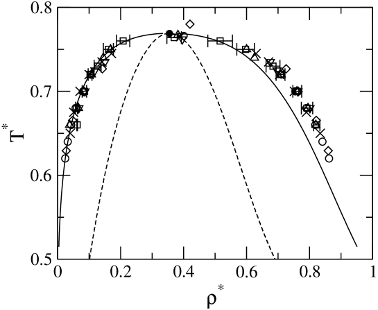
Figure 1: Liquid-vapor coexistence curve and critical point of the SW fluid of width $\delta=0.25$ in the density-temperature plane. Solid line: SCOZA. Full circle: SCOZA critical point. Squares with error bars: simulation data by Vega et al. vega . Diamonds: simulation data by Elliott et al. hu . Triangles: simulation data by Liu et al. liu Inverted triangles: simulation data by del Río at al. rio . Circles: simulation data by Orea et al. orea . Crosses: simulation data by Pagan et al. pagan . The SCOZA spinodal has also been shown by the dashed line.

The critical temperature and density predicted by the SCOZA are $T_{c}^{*}=0.769$, $\rho_{c}^{*}=0.355$. These values are close, but not identical to those found in paschinger for the same value of $\delta$, namely $T_{c}^{*}=0.761$, $\rho_{c}^{*}=0.343$. The difference is to be traced back to both the somewhat lower value of $\rho_{0}$ used there, $\rho_{0}^{*}=1.15$, and the fact that the boundary condition at $\rho_{0}$ was imposed on $\partial^{2}u/\partial\rho^{2}$ rather than $u$. As observed in Sec. II, we found that this enhanced the sensitivity of the results to the choice of the approximation used at $\rho_{0}$, namely, the HTA in the case of paschinger . The main difference between the two coexistence curves is that the liquid branch of the present one is slightly shifted to higher densities with respect to that obtained in paschinger . Nevertheless, the two curves are close to each other, and the comparison with the simulation results vega ; hu ; liu ; rio ; pagan ; orea shown in Fig. 1 confirms the trend already found there, i.e., the liquid branch of the SCOZA coexistence curve underestimates the simulation results. The different simulations reported in the figure are enough consistent with one another to indicate that this is indeed an inaccuracy of the SCOZA. The critical temperature is in good agreement with most simulation results vega ; liu ; rio ; pagan ; orea , while the critical density is underestimated with respect to all of them, although it lies within the error-bar given in vega , and the discrepancy is generally smaller than that observed on the liquid branch of the coexistence curve.

Figures 2, 3 show the SCOZA spinodal and coexistence curves respectively for $\delta=0.15$ and $\delta=0.1$, together with simulation data for the coexistence curve and the critical point skibinsky ; pagan ; liu ; orea ; largo ; duda . The SCOZA results were again obtained using the non-linear ORPA as the boundary condition at $\rho_{0}$, and setting $\rho_{0}^{*}=1.4$.

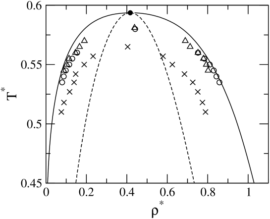
Figure 2: Same as Fig. 1 for $\delta=0.15$. Solid line: SCOZA. Full circle: SCOZA critical point. Circles: simulation data by Orea et al. orea . Crosses: simulation data by Pagan et al. pagan . Triangles: simulation data by Liu et al. liu . Dashed line: SCOZA spinodal.

Unlike what found for $\delta=0.25$, the coexistence curve of the SCOZA is wider than most simulation predictions. This behavior is largely due to the fact that now the SCOZA critical temperature is appreciably higher than the simulation ones.

As a general remark, the overall agreement with the phase diagram predicted by the SCOZA appears to be worse than that found for HCY potentials of comparable range scozayuk4 ; foffi ; scozaorea , although for $\delta=0.15$ and $\delta=0.1$ a quantitative assessment of the performance of the SCOZA is difficult, because of the rather large discrepancies shown by different simulations.

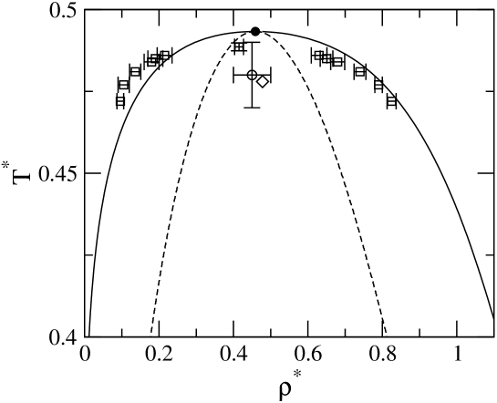
Figure 3: Same as Fig. 1 for $\delta=0.1$. Solid line: SCOZA. Full circle: SCOZA critical point. Squares with error bars: simulation data by Duda duda . Circle with error bars: simulation critical point by Skibinsky et al. skibinsky . Diamond: simulation critical point by Largo et al. largo . Dashed line: SCOZA spinodal.

A perhaps more conclusive comparison can be made with the recent simulation results for the critical point obtained in largo , some of which have been reported in Tab. 1 together with the SCOZA predictions. These indicate that the SCOZA for the SW fluid underestimates $\rho_{c}$, the discrepancy on $\rho_{c}$ being larger than that on $T_{c}$. In a previous investigation of the SCOZA for narrow HCY fluids scozaorea , $\rho_{c}$ was again found to deviate from simulations more than $T_{c}$, although in that case $\rho_{c}$ was overestimated by the SCOZA.

		SCOZA				MC
$\delta$		$T_{c}^{*}$		$\rho_{c}^{*}$		$T_{c}^{*}$		$\rho_{c}^{*}$
$0.8$		$1.953$		$0.247$		$1.940$		$0.263$
$0.5$		$1.211$		$0.272$		$1.220$		$0.310$
$0.3$		$0.850$		$0.328$		$0.847$		$0.376$
$0.2$		$0.683$		$0.382$		$0.667$		$0.421$
$0.1$		$0.493$		$0.459$		$0.4780$		$0.478$

Table 1: Critical temperature and density of the SW fluid for several values of the well width $\delta$, as obtained by the SCOZA and Monte Carlo (MC) numerical simulations performed in largo . According to the estimate given in largo for the case $\delta=0.05$ (not reported here), the errors in the MC critical parameters are about $\pm 0.14\%$ for $T_{c}^{*}$ and $\pm 1.56\%$ for $\rho_{c}^{*}$.

A qualitative feature common to the SCOZA phase diagrams shown in Figs. 1, 2, 3 is that the coexistence curve is much wider then the spinodal curve, so that even at densities near the critical one, and a fortiori at low or high densities, there is a sizable temperature interval where the fluid may survive in a single phase as a metastable state, before spinodal decomposition sets in. According to this, in the experimental practice one should be circumspect before using spinodal decomposition to identify equilibrium phase separation on the assumption that the coexistence and spinodal curves run close to each other. In fact, according to the SCOZA they do not, especially at the low volume fractions that are frequently considered in experiments on colloidal dispersions.

For wells such that $\delta\leq 0.05$, the dependence of the SCOZA on the high-density boundary condition becomes so strong, that the results do not show any clear trend towards saturation in the region $\rho_{0}^{*}\leq 1.4$. It is possible that this could be achieved by moving $\rho_{0}$ to even higher values, bigger than that corresponding to the physical close packing. However, with the fully numerical algorithm considered here we failed to obtain solutions of Eqs. (6), (7) beyond close packing, because in this regime the correlation functions become very singular, and even the prescription described in Appendix A proved insufficient, at least for the number of points in the numerical Fourier transform that can be handled in practice. Therefore, the results that we have obtained for $\delta\leq 0.05$ cannot be considered meaningful.

It is worthwhile pointing out that the sensitivity on the boundary condition at high density is much stronger for the SW potential considered here than for the HCY potential. In order to compare the two cases, it is useful to resort to the NF mapping noro mentioned in Sec. I, according to which a fluid of hard-core particles of diameter $\sigma$ with a given attractive tail potential at reduced temperature $T^{*}$ can be mapped into a SW fluid with the same $\sigma$, and a range determined so that its second virial coefficient $B_{2}(T)$ coincides with that of the original fluid for $T=T^{*}$. We remark that here this mapping is used without any assumption as to the behavior of the system for interactions of vanishing range, so its use is fully legitimate also within the SCOZA. A HCY fluid with inverse-range parameter $z=5.5$ at $T^{*}=0.48$, which is the critical value according to the SCOZA, should then be equivalent to a SW fluid with $\delta=0.1$ at the same $T^{*}$. The SCOZA critical temperature of this SW, $T_{c}^{*}=0.49$, is indeed close to that of the HCY, in agreement with the prediction from the mapping, while the difference between the critical densities, $\rho_{c}^{*}=0.459$ for the SW and $\rho_{c}^{*}=0.427$ for the HCY, although larger, is still below $10\%$. However, for the HCY fluid setting $\rho_{0}^{*}=1$ is sufficient to obtain a stable critical point, while for the SW $\rho_{0}^{*}$ must be set at a substantially higher value, $\rho_{0}^{*}=1.4$.

Further insight into the difference between the two potentials is obtained by checking the behavior of the effective range $\delta$ of the HCY below $T_{c}$: we find that, as the temperature decreases, the effective range also decreases. As a consequence, for $T<T_{c}$ it should be possible to map the densities at coexistence of the HCY fluid into those of a SW fluid at the same $T^{*}$, but with a lower $T_{c}^{*}$, i.e., at a higher rescaled temperature $T/T_{c}$. This implies that, according to the NF mapping, the coexistence curve of the HCY fluid in the $T$-$\rho$ plane should be narrower than that of the “equivalent” SW at $T_{c}^{*}$.

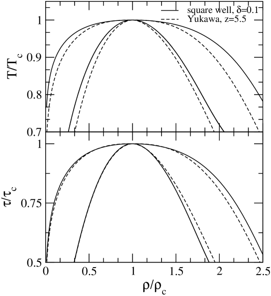
Figure 4: Solid line: SCOZA coexistence (outer) and spinodal (inner) curves for a SW fluid of width $\delta=0.1$. Dashed line: same for a HCY fluid with inverse-range parameter $z=5.5$. The upper panel shows the curves in the temperature-density plane, with both variables rescaled by their critical values. In the lower panel the rescaled temperature has been replaced by the rescaled stickiness parameter $\tau/\tau_{c}$ baxter . Note how the curves for the two potentials get closer in the latter case.

That this is actually the case is shown in the upper panel of Fig. 4, where the coexistence and spinodal curves of the HCY fluid with $z=5.5$ and the SW fluid with $\delta=0.1$ have been plotted using rescaled temperatures $T/T_{c}$ and densities $\rho/\rho_{c}$. It is evident that the SW coexistence curve is appreciably wider, especially when the liquid branch is considered. It is also worthwhile considering the behavior of the coexistence and spinodal curves when the temperature is replaced by $B_{2}(T)$, or equivalently by the stickiness parameter $\tau$ obtained by replacing $B_{2}^{\rm SHS}$ with $B_{2}(T)$ in Eq. (3). The NF mapping predicts that, with this choice of the temperature-like variable, the phase diagram of narrow attractive potentials should become universal. The two fluids considered here do give similar values for $\tau$ at the critical point, namely, $\tau_{c}=0.115$ for the SW and $\tau_{c}=0.107$ for the HCY. If the rescaled temperature $T/T_{c}$ is replaced by the rescaled stickiness $\tau/\tau_{c}$, as in the lower panel of Fig. 4, the vapor branches of the coexistence and spinodal curves become nearly coincident, and the discrepancy between the liquid branches of the coexistence curve becomes substantially smaller, although the SW still gives a wider curve. Quite curiously, the situation with the liquid branches of the spinodals is reversed with respect to that shown in the upper panel, i.e., as a function of $\tau$ the SW spinodal is narrower than the HCY spinodal, while as a function of $T$ it is wider. On the basis of the above considerations, the sensitivity of the SW potential to the high-density boundary condition may depend at least in part on the fact that its phase diagram is shifted towards higher densities than those of a HCY fluid of equivalent range.

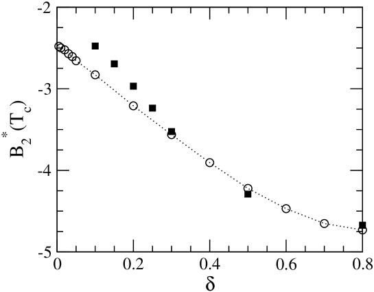
Figure 5: Reduced second virial coefficient of the SW fluid at the critical temperature $B_{2}^{*}(T_{c})$ as a function of the well width $\delta$. Squares: SCOZA. Circles: simulation results by Largo et al. largo . The dotted line is a guide to the eye.

The behavior of $B_{2}(T_{c})$, shown in Fig. 5, is in semi quantitative agreement with the simulation results largo . In both cases, the $B_{2}(T_{c})$ increases as $\delta$ decreases. However, because of the impossibility to obtain meaningful results for the critical point of narrow wells such that $\delta\leq 0.05$, we are not able to say what the fate of the SCOZA $B_{2}(T_{c})$ will be in the limit $\delta\to 0$, namely, if it will tend to a finite value as predicted by the simulations miller ; largo . The arguments put forth in Sec. IV rather suggest that the SCOZA would not yield a finite value of $B_{2}(T_{c})$ for vanishing attraction range.

We now briefly consider some thermodynamic properties of the SW fluid. Figure 6 displays the compressibility factor $\beta P/\rho$ and the internal energy per particle $U^{*}$ for $\delta=0.1$ along the isotherms $T^{*}=2$ and $T^{*}=1$, compared with simulation results bergenholtz . The agreement is very satisfactory both at low and high density, although it is fair to point out that the temperatures at which the simulations were performed can be considered quite high, since even $T^{*}=1$ is still more than twice the expected critical value reported in Tab. 1.

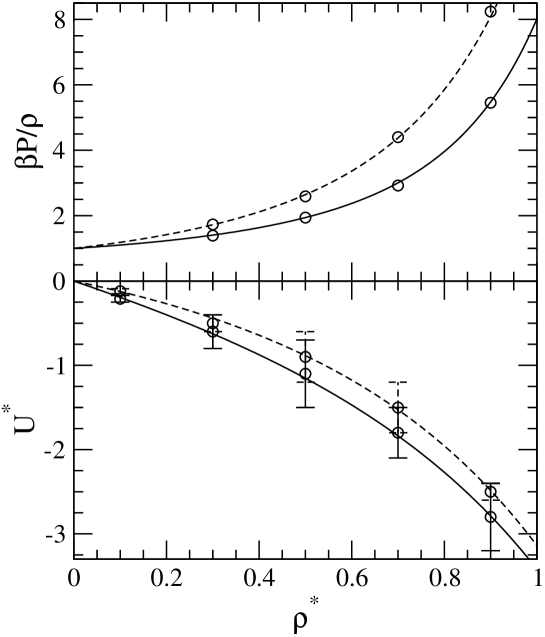
Figure 6: Compressibility factor $\beta P/\rho$ (upper panel) and excess internal energy per particle $U^{*}$ (lower panel) of the SW fluid with $\delta=0.1$. Solid line: SCOZA for $T^{*}=1$. Dashed line: SCOZA for $T^{*}=2$. Circles: simulation results at the same temperatures bergenholtz .

A comparison encompassing temperatures closer to $T_{c}$ is shown in Fig. 7, where $\beta P/\rho$ and $U^{*}$ for $\delta=0.25$ are shown along the isochore $\rho^{*}=0.42$ as a function of the inverse temperature $\beta$, and compared with simulation results kiselev . The agreement is again quite good down to the lowest temperature attainable by the SCOZA, i.e., that at which the isochore hits the high-density branch of the spinodal curve. Inspection of Fig. 2 of kiselev suggests that the simulation data at the lowest temperatures, roughly for $\beta\gtrsim 1.33$, would correspond to unstable states in the thermodynamic limit.

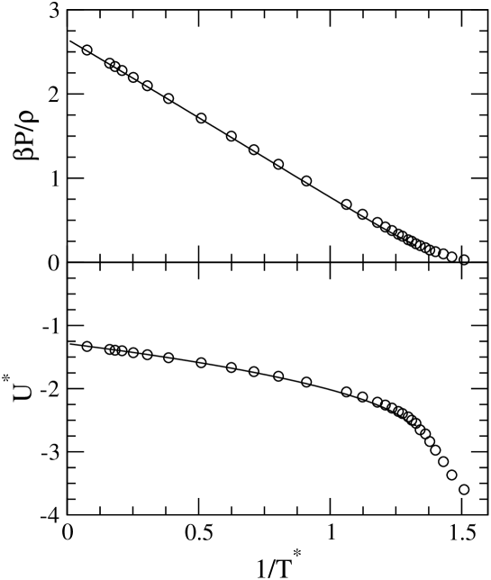
Figure 7: Compressibility factor $\beta P/\rho$ (upper panel) and excess internal energy per particle $U^{*}$ (lower panel) of the SW fluid with $\delta=0.25$ and $\rho^{*}=0.42$. Solid line: SCOZA. Circles: simulation results kiselev .

It is also worthwhile examining how the present theory performs for the correlations of the fluid. Figure 8 shows the structure factor $S(k)$ for a SW with $\delta=0.1$ and two different states, one at moderate density $\rho^{*}=0.5$ and relatively high temperature $T^{*}=2$, and another at lower density $\rho^{*}=0.229$ and temperature $T^{*}=0.5$ near the critical value. In both cases, the SCOZA reproduces quite accurately the simulation results shukla .

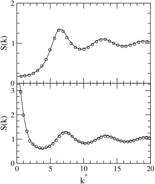
Figure 8: Structure factor of the SW fluid with $\delta=0.1$ for $T^{*}=2$, $\rho^{*}=0.5$ (upper panel) and $T^{*}=0.5$, $\rho^{*}=0.229$ (lower panel). Solid line: SCOZA. Circles: simulation data by Shukla et al. shukla extracted from their Figs. 6 and 8.

The correlations in real space are considered in Fig. 9, where the radial distribution function $g(r)$ predicted by the SCOZA, again for $\delta=0.1$ and $T^{*}=0.5$, is compared with simulation data santos at the densities $\rho^{*}=0.2$, $\rho^{*}=0.4$, $\rho^{*}=0.8$.

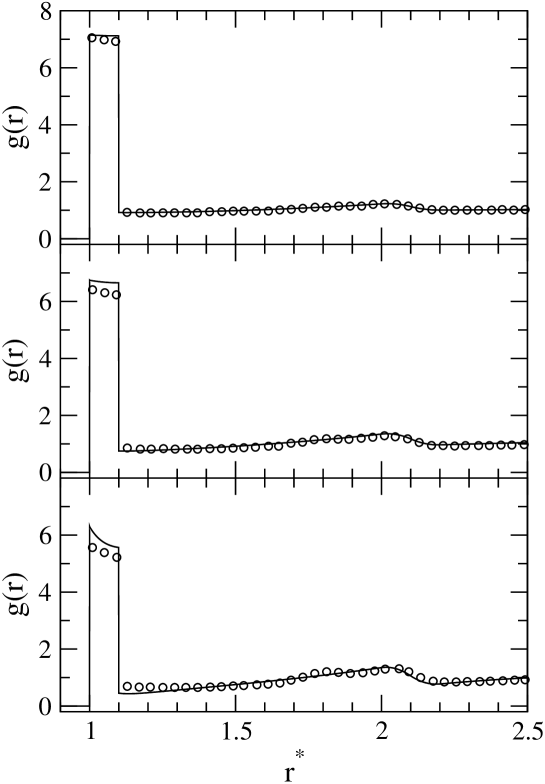
Figure 9: Radial distribution function of the SW fluid with $\delta=0.1$ for $T^{*}=0.5$ and $\rho^{*}=0.2$ (top panel), $\rho^{*}=0.4$ (central panel), $\rho^{*}=0.8$ (bottom panel). Solid line: SCOZA. Circles: simulation data by Largo et al. santos extracted from their Fig. 6.

At low density, the theory agrees closely with the simulation, both inside and outside the well region. This is not surprising since, as pointed out in Sec. I, the SCOZA for the SW potential becomes exact at low density, while this is not the case for other tail interactions. On the other hand, as $\rho$ is increased the SCOZA overestimates both the contact value $g(\sigma^{+})$ of $g(r)$, and the amplitude of the discontinuity at the well boundary $\xi\equiv(1+\delta)\sigma$. This also testifies the quite special status of the SW potential within the SCOZA: in fact, for the HCY potential scozayuk4 the SCOZA was found to underestimate $g(\sigma^{+})$, as one would expect from a theory whose $c(r)$ is linear in the perturbation potential. In the present case, the behavior at high density is instead reminiscent of that of the “non-linear ORPA” studied in orpanl . Another feature worth attention is the hump displayed by the simulation $g(r)$ for $\rho^{*}=0.8$ and $r^{*}\simeq 1.8$, which is the precursor of the discontinuity for $r^{*}=\sqrt{3}$ displayed by $g(r)$ in the sticky limit miller2 ; malijevsky . This is not reproduced by the SCOZA, most likely because of the assumption implied by Eq. (7) that $c(r)$ has the same range as the potential.

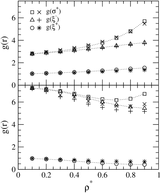
Figure 10: Radial distribution function of the SW fluid with $\delta=0.1$ for $r\to\sigma^{+}$, $r\to\xi^{-}$, $r\to\xi^{+}$, where $\xi\equiv(1+\delta)\sigma$ is the value of $r$ beyond which the potential vanishes. Squares, triangles, and circles represent the SCOZA results for $g(\sigma^{+})$, $g(\xi^{-})$, and $g(\xi^{+})$ respectively. Crosses, pluses, and starbursts represent the simulation data obtained by Largo et al. santos for the same quantities. Dotted lines are a guide to the eye. Upper panel: $T^{*}=1$ isotherm. Lower panel: $T^{*}=0.5$ isotherm.

A closer look at the $g(r)$ at contact and at the well boundary is given in Fig. 10, where $g(\sigma^{+})$, $g(\xi^{-})$, $g(\xi^{+})$ for $\delta=0.1$ are shown along the isotherms $T^{*}=0.5$ and $T^{*}=1$. As one may expect, the aforementioned discrepancy with the simulation data that sets out at large $\rho$ becomes less severe as $T$ is increased, the results for $T^{*}=1$ being in good agreement with the simulation santos even at the highest $\rho$ considered.

IV The sticky limit of the SCOZA

As discussed in Sec. III, the numerical solution of the SCOZA for the SW potential developed here becomes unpredictive for wells such that $\delta\leq 0.05$, still considerably wider than the HCY potentials that were considered in foffi ; scozaorea . However, in the limit $\delta\to 0$ it is possible to study the behavior of the SCOZA by adopting a different standpoint, namely, by imposing thermodynamic consistency on the solution to Eqs. (6), (7) after the limit $\delta\to 0$ has been taken. The clue to this procedure lies in the observation made in gazzillo that in the limit $\delta\to 0$, any OZ closure like Eq. (7), such that one has $h(r)=-1$ for $r<\sigma$ and $c(r)=0$ for $r>(1+\delta)\sigma$, gives a fixed form for $c(r)$:

$$c(r)=\left\{-\,\frac{\eta\lambda}{r^{*}}-a^{2}+\eta\left[6(a+b)^{2}-a\lambda\right]r^{*}-\frac{\eta a^{2}}{2}{r^{*}}^{3}\right\}\Theta(1-r^{*})+\frac{\lambda}{12}\,\delta(r^{*}-1)\,,$$ (26)

where $\Theta(x)$ and $\delta(x)$ are respectively the Heaviside and Dirac functions of argument $x$, and we have set $\eta\equiv\pi\rho\sigma^{3}/6$. The quantities $a$ and $b$ are given by

$$a = \frac{1+2\eta}{(1-\eta)^{2}}-\frac{\lambda\eta}{1-\eta}\,,$$ (27)

$$b = -\frac{3\eta}{2(1-\eta)^{2}}+\frac{\lambda\eta}{2(1-\eta)}\,.$$ (28)

Therefore, in the limit $\delta\to 0$ all the specific features of the OZ closure considered are conveyed into a single, state-dependent parameter $\lambda$. The latter is related to the stickiness parameter $\tau$ defined in Eq. (3) and to the contact value of the cavity function $y(r)=g(r)\exp{[\beta v(r)]}$ by the expression

$$\lambda=\frac{y({\sigma})}{\tau}\,.$$ (29)

By applying the compressibility rule (9) to Eq. (26), one obtains

$$\frac{1}{\,\chi_{\rm red}}=a^{2}\,,$$ (30)

whereas the energy route gives watts

$$\frac{\beta A}{N}=\frac{\beta A_{\rm HS}}{N}-\eta\int_{\tau}^{+\infty}\!\!d\tau^{\prime}\,\frac{\lambda(\eta,\tau^{\prime})}{\tau^{\prime}}\,.$$ (31)

If the form of $\lambda(\eta,\tau)$ obtained by the PY closure is substituted into Eqs. (26)-(31), the aforementioned solution of the SHS model due to Baxter baxter is recovered. On the other hand, as discussed in detail in gazzillo , different choices for $\lambda$ are also possible. Since one of the most problematic features of the original SHS model is its lack of thermodynamic consistency, it is tempting to determine $\lambda$ via the SCOZA, thus enforcing consistency between the compressibility and energy routes given by Eqs. (30), (31). If we introduce the quantities

$$\Lambda = \eta^{2}\lambda\,,$$ (32)

$$t = \frac{1}{\tau}\,,$$ (33)

the SCOZA equation reads

$${\cal D}(\eta,t)\,t\frac{\partial\Lambda}{\partial t}=\frac{\partial^{2}\!\Lambda}{\partial\eta^{2}}\,,$$ (34)

where ${\cal D}(\eta,t)$ is given by

$${\cal D}(\eta,t)=2\,\frac{\eta\,(1+2\eta)-(1-\eta)\Lambda}{[\,\eta\,(1-\eta)]^{3}}\,.$$ (35)

The PDE (34) can be solved numerically by the finite-difference scheme described in the Appendix of scozaising , or the similar one given here by Eq. (48); unlike in the case of non vanishing $\delta$, the diffusion coefficient is given explicitly by Eq. (35), so there is no need to evaluate it by finite differences as in Eq. (49). As usual, for the problem to be completely specified, Eq. (34) must be complemented with the initial and boundary conditions. As for the initial condition, we observe that the numerical integration cannot be started exactly from $t=0$, because for this value of $t$ the diffusion coefficient $1/(t{\cal D})$ would become infinite. Instead, the integration was started from a small, but non null $t_{0}>0$, using as the initial condition for $\Lambda$ the leading term in an expansion in powers of $t_{0}$

$$\Lambda(\eta,t_{0})\simeq t_{0}\,\varphi(\eta)\,.$$ (36)

By substituting Eq. (36) into Eq. (34) we find that the $\eta$-dependent term $\varphi(\eta)$ must satisfy the ordinary differential equation 

$$\frac{d^{2}\varphi}{d\eta^{2}}=2\,\frac{1+2\eta}{\eta^{2}(1-\eta)^{3}}\,\varphi\,.$$ (37)

This is solved numerically with the conditions

$$\varphi(0)=\left.\frac{d\varphi}{d\eta}\right|_{\eta=0}\!\!=0\,,$$ (38)

$$\left.\frac{d^{2}\varphi}{d\eta^{2}}\right|_{\eta=0}\!\!=2\,,$$ (39)

that follow from Eqs. (29), (32), (36) and the property gazzillo

$$\lim_{\eta\to 0}y(\sigma)=1\,.$$ (40)

We have verified a posteriori that the numerical solution of Eq. (34) is virtually independent of the particular choice of $t_{0}$, as long as the latter is sufficiently small. Equations (29), (32), also imply for the low-density boundary condition

$$\Lambda(\eta=0,t)=0\mbox{\hskip 56.9055pt for every $t$.}$$ (41)

As observed in Sec. II, the choice of the high-density boundary condition entails a certain amount of arbitrariness. A natural possibility is using for $\lambda$ the expression $\lambda_{\rm Bax}$ obtained by the analytical solution of the SHS model within the PY approximation baxter :

$$\Lambda(\eta_{0},t)=\eta_{0}^{2}\lambda_{\rm Bax}(\eta_{0},t)\mbox{\hskip 56.9055pt for every $t$},$$ (42)

where $\eta_{0}$ denotes the position of the high-density boundary. Quite disappointingly, although perhaps not surprisingly, the outcome of the numerical integration of Eq. (34) with the initial and boundary conditions given by Eqs. (36), (41), (42) suffers from the same problem experienced in Sec. III for wells of non vanishing width, namely, a strong dependence of the results on the position of $\eta_{0}$. This is illustrated in Fig. 11, where the inverse reduced compressibility $1/\chi_{\rm red}$ obtained for different choices of $\eta_{0}$ has been plotted along the isotherm $\tau=0.11$, which is close to the critical one according to numerical simulations miller . For the solution to be deemed reliable, the various curves, at least for $\eta_{0}$ greater than a certain threshold, ought to lie near one another — a requirement that is manifestly not satisfied. Some of the isotherms are not even consistent with $\tau=0.11$ being close to the expected critical value. We have also verified that this state of affairs is not changed by different choices of the high-density boundary condition.

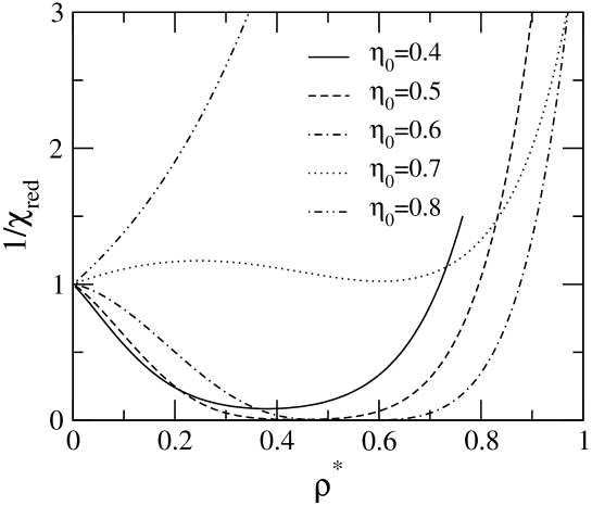
Figure 11: Inverse reduced compressibility $1/\chi_{\rm red}$ of the SHS fluid as a function of the reduced density $\rho^{*}$ as found via the SCOZA equation (34) with a high-density boundary condition computed in the PY approximation baxter . The different lines refer to the boundary packing fractions $\eta_{0}=\pi\rho_{0}^{*}/6$ given in the legend. The stickiness parameter is set at $\tau=0.11$, which is close to the critical value according to numerical simulations miller .

We can, however, resort to a different method to solve Eq. (34), that does not require the high-density boundary to be specified. This is made possible by the fact that, unlike in the case of wells of non vanishing width discussed in Secs. II, III, the diffusion coefficient of Eq. (34) is known explicitly as a function of $\eta$ and $\tau$. Let us assume that $\Lambda$ can be expressed as a power series in $t$

$$\Lambda(\eta,t)=\sum_{n=1}^{\infty}t^{n}\omega_{n}(\eta)\,,$$ (43)

where the zeroth-order term has been omitted, since $\Lambda$ must vanish for $t\to 0$. By inserting Eq. (43) into Eq. (34) and equating the terms of the same degree in $t$, Eq. (34) is replaced by an infinite set of ordinary differential equations:

$$\frac{d^{2}\omega_{n}}{d\eta^{2}}=2n\frac{1+2\eta}{\eta^{2}(1-\eta)^{3}}\,\omega_{n}-\frac{2}{\eta^{3}(1-\eta)^{2}}\sum_{j=1}^{n-1}j\,\omega_{j}\omega_{n-j}\,,$$ (44)

which gives back Eq. (37) for $n=1$. Since this set contains only backward references, it can be integrated numerically to any desired order $\bar{n}$. Only the low-density behavior of $\omega_{n}$ is required. Specifically, one needs the values of $\omega_{n}$, $d\omega_{n}/d\eta$, and $d^{2}\omega_{n}/d\eta^{2}$ at $\eta=0$ for $n\leq\bar{n}$. If it is assumed that $\omega_{n}$ can be expanded in power series of $\eta$, it is found that for $n>6$ all the above quantities are in fact vanishing, while for $n\leq 6$ they can be obtained from exact diagrammatic expansions available in the literature gazzillo ; post . Unfortunately, the radius of convergence $t_{\rm R}$ of the series (43) corresponding to most values of the packing fraction $\eta$ comes out to be too small for it to be of direct usefulness. This is apparent from Fig. 12, which shows how $t_{\rm R}$ rapidly decreases as the density is increased. In particular, at the critical value of $t$ predicted by simulations miller , $\rho^{*}$ should be well below $0.2$ to obtain convergence.

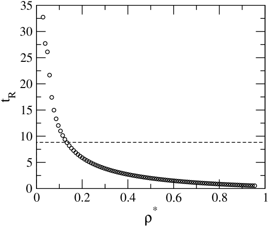
Figure 12: Radius of convergence $t_{\rm R}$ of the power series (43), estimated by means of the ratio convergence test, as a function of the reduced density $\rho^{*}$. The horizontal dashed line marks the value of the inverse stickiness $t$ corresponding to the critical point according to numerical simulations miller .

This is again disappointing, yet not uncommon: a power series obtained as a formal solution of a differential equation may easily turn out to be divergent. In those cases, one can try a resummation technique in order to provide an analytic meaning to such a divergent series. To this end, we have employed Borel summation method kawai , whereby one starts from the exact equality

$$\Lambda(\eta,t)=\sum_{n=1}^{\infty}n!\frac{t^{n}}{n!}\,\omega_{n}(\eta)=\frac{1}{t}\sum_{n=1}^{\infty}\int_{0}^{+\infty}\!\!ds\,e^{-s/t}\,\frac{{s}^{n}}{n!}\,\omega_{n}(\eta)$$ (45)

and formally interchanges the series and the integral operators to obtain

$$\Lambda_{\rm B}(\eta,t)=\frac{1}{t}\int_{0}^{+\infty}\!\!ds\,e^{-s/t}\,\tilde{\Lambda}(\eta,s)\,,$$ (46)

where $\tilde{\Lambda}(\eta,s)$ is the regularized power series

$$\tilde{\Lambda}(\eta,s)=\sum_{n=1}^{\infty}\frac{s^{n}}{n!}\,\omega_{n}(\eta)\,,$$ (47)

that has an improved radius of convergence because of the factorial in the denominator. Where the original series is convergent, the two functions $\Lambda$ and $\Lambda_{\rm B}$ are in fact identical. The latter, however, yields a finite value in a much larger domain, providing the analytic continuation of the function defined by the original series. If one is willing to trust the Borel sum $\Lambda_{\rm B}$ in this enlarged region, then a puzzling result is found: the liquid-vapor phase transition disappears, at least for reasonable values of the packing fraction and temperature. In Fig. 13 the inverse reduced compressibility of the fluid $1/\chi_{\rm red}$ is shown as a function of $t$ along the $\eta=0.25$ isochore.

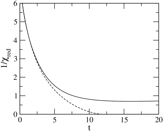
Figure 13: Inverse reduced compressibility $1/\chi_{\rm red}$ of the SHS fluid as a function of the inverse stickiness $t$ along the $\eta=0.25$ isochore. The compressibility route of the PY approximation (dashed line) predicts the compressibility to diverge at $t\simeq 12$. According to the solution of Eq. (34) evaluated by means of the Borel summation method (solid line), the isochore does not cross the spinodal at all.

While the compressibility route of the PY approximation predicts the compressibility to diverge around $\tau\simeq 0.08$, the solution of Eq. (34) evaluated by means of Borel summation method gives instead a finite $\chi_{\rm red}$ even if the temperature is lowered further. This result is qualitatively similar to that found by direct numerical integration of Eq. (34) when the high-density boundary $\eta_{0}$ is pushed to (unphysically) high values, but is clearly at odds not only with the PY solution of the SHS model baxter , but also with the simulation results miller . The present investigation supports the conclusion that in the limit of vanishing well width $\delta\to 0$, the SCOZA critical temperature decreases too rapidly to give a finite value of $B_{2}(T_{c})$, so that $B_{2}(T)$ or, equivalently, the stickiness $\tau$, do not represent a convenient way to measure the temperature in this limit. Imposing thermodynamic consistency on the SHS model does not lead to a better quantitative agreement with simulation compared to the highly inconsistent PY solution, but merely makes the liquid-vapor transition disappear.

V Conclusions

We have performed an investigation of the SCOZA for SW potentials, focused on the regime of narrow wells which is the most relevant for the modelization of colloidal particles. This study was prompted by the lack of a theory able to account quantitatively for the liquid-vapor phase transition in a system of sticky hard spheres: in the well known and widespreadily used PY approximation baxter , the various routes to the thermodynamics of the fluid are inconsistent with one another, and agree only qualitatively with the results of computer simulation miller . On the other hand, for HCY potentials the SCOZA can be solved semi-analytically, and has already been usefully applied to narrow-range tails foffi ; scozaorea . The rationale for turning to the SW potential within the SCOZA is that this interaction has the unique feature of having the SCOZA become exact at low density, thereby recovering the correct $B_{2}(T)$ which plays such an important role for narrow interactions.

However, the results presented here show that this peculiarity turns more into a liability than an asset. For wells of non vanishing width $\delta$, after extending the study already made in paschinger to (slightly) smaller $\delta$, we cannot but confirm the conclusions of that work, namely: i) the results are found to be very sensitive to the boundary condition at high density that is needed to integrate the SCOZA PDE, actually much more so than in the case of HCY potentials of comparable range. Such an undesired feature can be tamed by pushing the density of the boundary to very high values, but this has the effect of making the numerical solution of the PDE unfeasible for $\delta\lesssim 0.05$. ii) In the range of $\delta$ for which meaningful results can be extracted, the overall agreement with simulation data, at least for the phase diagram, is actually worse than what was found for the HCY potential scozayuk4 ; foffi ; scozaorea , although a sharp assessment of the performance of the SCOZA is made difficult by the considerable discrepancies between different simulations.

If the sticky limit is taken from the outset, and subsequently thermodynamic consistency is imposed, the SCOZA PDE is obtained explicitly in closed form, but the high-density boundary problem is again found to be looming. If the PDE is turned into an infinite set of ordinary differential equations and the low-density behavior alone is imposed, the liquid-vapor phase boundary disappears altogether. This supports the conclusion that as the attractive potential range vanishes, the SCOZA critical temperature will decrease more rapidly than what is necessary to yield a finite $B_{2}(T_{c})$.

Stating that the SCOZA is inadequate for SW interactions in the sticky limit is merely an observation, and does not shed any light on the reason behind the fact. In this respect, one should recall the result of Stell stell mentioned in Sec. I, who showed that the SHS model is strictly speaking ill-defined if a class of problematic configurations of particles is not ruled out, for instance by introducing a small amount of polidispersity into the system. Can it be that the (possibly more accurate) SCOZA approach exposes the malicious effect of the diverging clusters, which are simply neglected in the PY approximation? We regard this as unlikely, since the two approximations are quite similar in their handling of the correlation functions of the fluid, giving the same functional form for $c(r)$ in the sticky limit gazzillo . What we deem most probable, instead, is that the failure is a combined effect of the approximate closure (7) and the consistency requirement (8). Indeed, the closure is likely to miss a number of singular features, i.e., discontinuities and Dirac-$\delta$ peaks, that show up in the real correlation function miller2 ; malijevsky : the isothermal compressibility, being dependent on the volume integral of the same function, suffers from the same defect. On the contrary, the internal energy of the fluid depends on the contact value of the cavity function alone: when thermodynamic consistency is imposed, the latter has to compensate for the missing contributions, unnaturally pushing away the liquid-vapor phase boundary. We stress that at the moment this is a mere, untested hypothesis.

One may hope that the strong dependence of the results on the high-density boundary condition found for narrow SW potentials will become less drastic turning to a different form of the interaction. In fact, as observed above, for the HCY potential this unwelcome feature, albeit still there, is nevertheless much less pronounced. If this is actually the case, then the fully numerical solution of the SCOZA which has been developed here and the one previously developed in paschinger , could still be usefully applied to different forms of short-range potentials, not to mention the instance of interactions that are not of short range paschinger08 . Moreover, this solution could be helpful in the context of the renormalization-group based hierarchical reference theory (HRT) hrt , specifically for enforcing the core condition on $g(r)$ exactly (of course within the limit of numerical accuracy). In fact, in the smooth cut-off formulation of the HRT smooth , similarly to the SCOZA, this condition can be (and has been) implemented analytically for a HCY potential, but for a generic tail potential a numerical solution would again be needed. Also, this is always the case for the sharp-cut off HRT, irrespective of the form of the tail potential. In the latter theory, the core condition was implemented by introducing a number of approximations giri , which however affect the accuracy of this approach for short-range interactions scozayuk4 . A better procedure such as that developed here would certainly be more adequate.

As for the sticky limit, the results presented in this work suggest that, if thermodynamic consistency is to be employed as a way to improve upon the accuracy of the PY solution for the SHS potential (2), one should first get rid of the approximation common to the SCOZA and the PY equation: namely, that the contribution to the direct correlation function $c(r)$ due to the tail interaction $w(r)$ has the same range as $w(r)$ itself, and therefore vanishes wherever $w(r)$ does. In this respect, it is worthwhile recalling that the same approximation is used in conjunction with thermodynamic consistency not only in the SCOZA, but also in the HRT smooth . Therefore, if the combination of these ingredients is bound to become dangerous for vanishing attraction range, it is likely that this would affect the HRT as well, and that both the SCOZA and the HRT would benefit from a solution to this problem.

Appendix A Finite-difference discretization of the SCOZA PDE

Equation (11) is a nonlinear, diffusive-like PDE, where the quantity $D(\rho,u)$ given by Eq. (12) plays the role of the reciprocal of the diffusion coefficient. This PDE is discretized in the following way:

$$D(\rho_{j},u_{j}^{n+1/2})\,\frac{u_{j}^{n+1}-u_{j}^{n}}{\Delta\beta}=\frac{\rho_{j}}{2}\left[\frac{u_{j+1}^{n+1}-2u_{j}^{n+1}+u_{j-1}^{n+1}}{(\Delta\rho)^{2}}+\frac{u_{j+1}^{n}-2u_{j}^{n}+u_{j-1}^{n}}{(\Delta\rho)^{2}}\right]$$ (48)

and

$$D(\rho_{j},u_{j}^{n+1/2})=\frac{\left(\displaystyle{\frac{1}{\,\chi_{\rm red}}}\right)_{\!j}^{\!n+1}-\left(\displaystyle{\frac{1}{\,\chi_{\rm red}}}\right)_{\!j}^{\!n}}{u_{j}^{n+1}-u_{j}^{n}}\,,$$ (49)

where subscripts refer to the density $\rho$ and superscripts to the inverse temperature $\beta$ in the $(\rho,\beta)$ grid, so for instance $u_{j}^{n}\equiv u(\rho_{j},\beta_{n})$, and $\Delta\beta$, $\Delta\rho$ are respectively the inverse temperature and density steps used in the discretization.

Equation (48) has been solved by an implicit algorithm as follows: assuming that $u_{j}^{n}$ is known at a certain inverse temperature $\beta_{n}$ for every $\rho_{j}$, a guess for $u_{j}^{n+1}$ at the “new” temperature $\beta_{n+1}$ is given. This is determined by solving Eqs. (6), (7) with the approximation $K_{n+1}\simeq K_{n}+\Delta\beta$. The values of the inverse reduced compressibility $(1/\chi_{\rm red})_{j}^{n+1}$ corresponding to $u_{j}^{n+1}$ are then obtained by solving Eqs. (6), (7) at fixed density $\rho$ and internal energy $u$ via the method described in Sec. II and Appendix B. These values are used in Eq. (49) to obtain a trial value of $D(\rho_{j},u_{j}^{n+1/2})$, which is inserted into Eq. (48) to give a closed linear system of equations for $u_{j}^{n+1}$ at $\beta_{n+1}$. The values of $u_{j}^{n+1}$ thus obtained replace the initial guess, and the procedure is iterated until convergence is obtained. The $u_{j}^{n+1}$ at convergence are fed back into the algorithm to obtain $u_{j}^{n+2}$, and so on.

Appendix B Numerical optimization of the free energy functional

The most straightforward method to minimize the functional ${\cal S}$ defined by Eq. (23) is the steepest descent pastore , in which $\phi(r)$ and $K$ are updated iteratively by moving downhill in the direction opposite to that of the gradient of ${\cal S}$, namely

$$\phi_{l+1}(r) = \phi_{l}(r)-\lambda\,\Delta h_{l}(r)\mbox{\hskip 42.67912pt}r<\sigma\,,$$ (50)

$$K^{*}_{l+1} = K^{*}_{l}-\lambda\,\Delta V_{l}\,.$$ (51)

Here the indexes $l$, $l+1$ refer to the values of $\phi(r)$ and $K$ at two consecutive iterations, $\lambda$ (not to be confused with the state-dependent function $\lambda(\eta,\tau)$ introduced in Sec. IV) is a parameter determining the step size, and we have set

$$\Delta V=-\rho\!\int\!\!d^{3}{\bf r}\,\Delta h(r)w^{*}(r)+\Delta U^{*}\,.$$ (52)

The asterisks in Eqs. (51), (52) denote reduced quantities $K^{*}=K\epsilon$, $\Delta U^{*}=\Delta U/\epsilon$, $w^{*}(r)=w(r)/\epsilon$, where $\epsilon$ is the energy scale of $w(r)$. For the SW potential considered here, $\epsilon$ coincides with the well depth. Note that, for $\lambda$ to be the same dimensionless quantity in Eqs. (50) and (51), the differentiation of ${\cal S}$ has to be performed with respect to $K^{*}$ and $\sqrt{\rho}\phi(r)$.

To implement the algorithm, one starts from a guess for $K$ and $\phi(r)$ for $r<\sigma$, and determines $\phi(r)$ for $r>\sigma$ by the relation $\phi(r)=-Kw(r)$. In the numerical solution of the SCOZA, the guess at the inverse temperature $\beta_{n+1}$ and density $\rho_{j}$ was given by $\phi(r,\rho_{j},\beta_{n+1})\simeq\phi(r,\rho_{j},\beta_{n})$, $K(\rho_{j},\beta_{n+1})\simeq K(\rho_{j},\beta_{n})+\Delta\beta$. By switching to reciprocal space, the Fourier transform of $\Delta h(r)$ is determined via the OZ equation as

$$\Delta\hat{h}(k)=S_{\rm HS}(k)S(k)\hat{\phi}(k)\,,$$ (53)

where $S(k)$ is given by Eq. (19). Equation (53) is then inverse-transformed to give $\Delta h(r)$. This in turn is used to determine $\Delta V$ by Eqs. (10), (21), (52), and the $\Delta h(r)$ and $\Delta V$ thus obtained are used in Eqs. (50), (51) to update $\phi(r)$ and $K$ iteratively, until convergence is achieved.

As observed in pastore , a valuable improvement over the steepest descent is the conjugate gradient algorithm, which we have adopted here. In this method, the direction of descent at the step $l+1$ does not coincide with that of the gradient of ${\cal S}$ at step $l$, but is instead given by a linear combination of the gradients at all previous steps according to

$$\phi_{l+1}(r) = \phi_{l}(r)-\lambda\,\gamma_{l}(r)\mbox{\hskip 42.67912pt}r<\sigma\,,$$ (54)

$$K^{*}_{l+1} = K^{*}_{l}-\lambda\,\Gamma_{l}\,,$$ (55)

where $\gamma_{l}(r)$ and $\Gamma_{l}$ are defined by recurrence as pastore

$$\gamma_{l}(r) = \Delta h_{l}(r)+\alpha_{l}\gamma_{l-1}(r)\mbox{\hskip 42.67912pt}r<\sigma\,,$$ (56)

$$\Gamma_{l} = \Delta V_{l}+\alpha_{l}\Gamma_{l-1}\,,$$ (57)

with $\alpha_{0}=0$ and $\alpha_{l}$ for $l\geq 1$ given by

$$\alpha_{l}=\frac{\rho{\displaystyle\int}_{\!\!r<1}\!\!\!d^{3}{\bf r}\,\Delta h_{l}(r)\left[\Delta h_{l}(r)-\Delta h_{l-1}(r)\right]+\Delta V_{l}\left(\Delta V_{l}-\Delta V_{l-1}\right)}{\rho{\displaystyle\int}_{\!\!r<1}\!\!\!d^{3}{\bf r}\,\left[\Delta h_{l-1}(r)\right]^{2}+\left(\Delta V_{l-1}\right)^{2}}\,.$$ (58)

The numerator and denominator of Eq. (58) are scalar products of the form $\langle v_{l}|v_{l}-v_{l-1}\rangle$, $\langle v_{l-1}|v_{l-1}\rangle$ for the present case in which the “vector” $v_{l}$ consists of both the function $\sqrt{\rho}\Delta h_{l}(r)$ and the scalar $\Delta V$.

In the implementation of the algorithm, special attention has been paid to the choice of the parameter $\lambda$. In both the steepest descent and conjugate gradient methods, the optimal value of $\lambda$ at each step is determined by line minimization pastore . In the case of the conjugate gradient, this amounts to minimizing ${\cal S}[\phi_{l}(r)-\lambda\gamma_{l}(r),K^{*}_{l}-\lambda\Gamma_{l}]$ as a function of $\lambda$ for fixed $\phi_{l}(r)$, $\gamma_{l}(r)$, $K^{*}_{l}$, $\Gamma_{l}$. A possible way would be to use some method based on repeated evaluation of the functional ${\cal S}$ along the line $\phi_{l}(r)-\lambda\gamma_{l}(r)$, $K^{*}_{l}-\lambda\Gamma_{l}$. We found that this procedure is not recommended here for a number of reasons: first, it is not very efficient, since it requires many evaluation of ${\cal S}$ at each step. Second, at low temperature (see Sec. II) there is a density interval where the argument of the logarithm in Eq. (16) is not positive definite as a function of $k$, so great care has to be taken to prevent the functional ${\cal S}$ from being evaluated for these states pastore . Finally, there is a subtle, yet important reason related to the fact that, for the hard-core plus tail potential of Eq. (5), both $c(r)$ and $h(r)$ are discontinuous at $r=\sigma$, and display additional discontinuities if $w(r)$ is itself discontinuous, as in the case of the SW potential. In order to determine with good accuracy the Fourier transform of the correlation functions needed in the iterative procedure, it is then advisable to subtract off the discontinuous contribution before performing the numerical Fourier transform, and add to the result its Fourier transform determined analytically, as illustrated in Sec. II. However, when the functional $f_{\rm Ring}$ of Eq. (16) is discretized in the numerical calculation, the fundamental relations (17), (18) will hold rigorously if the numerical Fourier transforms of $\phi(r)$ and $\Delta h(r)$ are performed on the full functions, rather than just on their continuous part. As a consequence, the gain in accuracy achieved by splitting the functions to be transformed entails as a drawback that the solution of the Euler-Lagrange equation $\delta f_{\rm Ring}/\delta\phi(r)=0$ for $r<\sigma$ will not rigorously be anymore a minimum of $f_{\rm Ring}$ as defined by Eq. (16), and it is not obvious to us whether Eq. (16) can be modified so as to recover this property. This is one more reason why we chose to perform the minimization with respect to $\lambda$ by an algorithm which would not rely on the direct evaluation of ${\cal S}$, and hence of $f_{\rm Ring}$. Instead, we set $\psi(\lambda)={\cal S}[\phi_{l}(r)-\lambda\gamma_{l}(r),K^{*}_{l}-\lambda\Gamma_{l}]$, and determined the line minimum by solving the equation $d\psi/d\lambda=0$ with respect to $\lambda$. This was done by the Raphson-Newton method, namely starting from a guess value $\lambda_{0}$ and updating $\lambda$ recursively by the sequence

$$\lambda_{k+1}=-\,\frac{\left.{\displaystyle\frac{d\psi}{d\lambda}}\right|_{\lambda_{k}}}{\left.\displaystyle{\frac{d^{2}\psi}{d\lambda^{2}}}\right|_{\lambda_{k}}}\,.$$ (59)

In the present case we have

$$-\frac{d\psi}{d\lambda} \!=\! \int\!\!d^{3}{\bf r}\,\frac{\delta{\cal S}}{\delta\phi(r)}\,\gamma(r)+\frac{\partial{\cal S}}{\partial K^{*}}\,\Gamma\,,$$ (60)

$$\frac{d^{2}\psi}{d\lambda^{2}} \!=\! \int\!\!d^{3}{\bf r}\!\int\!\!d^{3}{\bf r}^{\prime}\,\frac{\delta^{2}{\cal S}}{\delta\phi(r)\delta\phi(r^{\prime})}\,\gamma(r)\gamma(r^{\prime})+2\Gamma\!\!\int\!\!d^{3}{\bf r}\,\frac{\partial}{\partial K^{*}}\frac{\delta{\cal S}}{\delta\phi(r)}\,\gamma(r)+\frac{\partial^{2}{\cal S}}{\partial{K^{*}}^{2}}\,\Gamma^{2}\,,$$ (61)

where we have understood that $\gamma(r)$ is set identically to zero for $r>\sigma$, and for brevity we have omitted the index $l$ in $\phi(r)$, $\gamma(r)$, $K^{*}$, $\Gamma$. All the derivatives of ${\cal S}$ are evaluated at $\phi_{l}(r)-\lambda_{k}\gamma_{l}(r)$, $K^{*}_{l}-\lambda_{k}\Gamma_{l}$, and are easily calculated by Eqs. (17), (18), (20), (22), (23). The quantities required are those already needed in Eq. (53) for $\Delta{\hat{h}}(k)$. Specifically, Eqs. (60), (61) become

$$\!\!\!\!\!-\frac{d\psi}{d\lambda} \!\!=\!\! \rho\!\!\int\!\!d^{3}{\bf r}\,\Delta h(r)\gamma(r)+\Gamma\Delta V\,,$$ (62)

$$\!\!\!\!\!\frac{d^{2}\psi}{d\lambda^{2}} \!\!=\!\! \rho\!\!\int\!\!\frac{d^{3}{\bf k}}{(2\pi)^{3}}\left[S(k)\hat{\gamma}(k)\right]^{2}\!-\!2\rho\Gamma\!\!\!\int\!\!\frac{d^{3}{\bf k}}{(2\pi)^{3}}\,S^{\,2}(k)\hat{w}^{*}(k)\hat{\gamma}(k)\!+\!\rho\Gamma^{2}\!\!\!\int\!\!\frac{d^{3}{\bf k}}{(2\pi)^{3}}\left[S(k)\hat{w}^{*}(k)\right]^{2}\,.$$ (63)

In practice, we have found that, for each conjugate gradient step (54), (55), (56), (57), a single Raphson-Newton step (59), (62), (63) for $\lambda$ is sufficient. Iterating Eq. (59) so as to get closer to the minimum of $\psi(\lambda)$ did not lead to any significant improvement in the overall speed of convergence of the algorithm.

We notice that at the critical point and on the spinodal curve, where the compressibility $\chi_{\rm red}$ diverges, the integrals that appear in Eq. (63) diverge as well, because $S^{\,2}(k)$ develops a non integrable singularity at $k=0$, see Eq. (19). In order to account for this behavior, for large values of $\chi_{\rm red}$ the contribution to the integrals in the small-$k$ domain is determined analytically by replacing $S(k)$ with its Ornstein-Zernike form $S(k)\simeq 1/(\chi_{\rm red}^{-1}+bk^{2})$, and evaluating the remainder of the integrand at $k=0$.

Appendix C Numerical calculation of the hard-sphere correlation function at high density

We start from the exact relation

$$h(r)=c(r)+\int\!\!\frac{d^{3}{\bf k}}{(2\pi)^{3}}\,e^{i{\bf k}\cdot{\bf r}}\,[\hat{h}(k)-\hat{c}(k)]=c(r)+\frac{\rho}{2\pi^{2}r}\int_{0}^{+\infty}\!\!dk\,\sin(kr)\frac{k\,\hat{c}^{2}(k)}{1-\rho\hat{c}(k)}\,,$$ (64)

where $\hat{c}(k)$ has been subtracted off from $\hat{h}(k)$ in order to make the integrand decrease more rapidly at large $k$. The function $\zeta(k)=k\,\hat{c}^{2}_{\rm HS}(k)/[1-\rho\hat{c}_{\rm HS}(k)]$, which is known analytically for the Waisman parametrization, is then sampled with a step $\Delta k\simeq 5\times 10^{-5}\sigma^{-1}$, much smaller than that used in the numerical Fourier transform, so that the “pseudo-Bragg” peaks can be included in the sampling. Each peak such that the structure factor exceeds the threshold value $S_{\rm HS}(k)=3$ is modeled by a Lorentzian $A/[1+\alpha^{2}(k-k_{0})^{2}]$, where the parameters $k_{0}$, $A$, $\alpha$ are determined so as to reproduce the position of the peak, its height, and its curvature. The sum of the Lorentzians is subtracted off $\zeta(k)$, resulting in a smooth function that can be transformed numerically without substantial loss of information, while the Fourier transform of the Lorentzians is determined analytically. In the present case in which $k_{0}\neq 0$ this cannot be done exactly, but we found that for narrow peaks such that $\alpha\gg 1$ like those considered here, a satisfactory approximation is given by

$$\frac{1}{2\pi^{2}r}\int_{0}^{+\infty}\!\!dk\,\frac{\sin(kr)}{1+\alpha^{2}(k-k_{0})^{2}} \simeq \frac{1}{2\pi\alpha r}\sin(k_{0}r)\,e^{-r/\alpha}$$

$$\mbox{}- \frac{1}{2\pi^{2}\alpha^{2}}\left\{\cos(k_{0}r){\rm Ci}(k_{0}r)-\sin(k_{0}r)\left[\frac{\pi}{2}-{\rm Si}(k_{0}r)\right]\right\}\,,$$

where ${\rm Si}(x)$ and ${\rm Ci}(x)$ are respectively the sine and cosine integrals defined as:

$${\rm Si}(x) = \int_{0}^{x}\!\!dt\,\frac{\sin(t)}{t}\,,$$ (66)

$${\rm Ci}(x) = \int_{0}^{x}\!\!dt\,\frac{\cos(t)-1}{t}+\ln(x)+\gamma\,,$$ (67)

where $\gamma=0.5772\ldots$ is Euler constant.

References

- (1) B. Götzelmann, R. Evans, and S. Dietrich, Phys. Rev. E 57, 6785 (1998); M. Dijkstra, R. van Roij, and R. Evans, Phys. Rev. Lett. 81, 2268 (1998); M. Dijkstra, R. van Roij, and R. Evans, Phys. Rev. Lett. 82, 117 (1999); M. Dijkstra, R. van Roij, and R. Evans, Phys. Rev. E 59, 5744 (1999); M. Dijkstra, J. M. Brader, and R. Evans, J. Phys.: Condens. Matter 11, 10079 (1999); R. Roth, R. Evans, and S. Dietrich, Phys. Rev. E 62, 5360 (2000); R. Roth, R. Evans, and A. A. Louis, Phys. Rev. E 64, 051202 (2001); M. Schmidt, H. Löwen, J. M. Brader, and R. Evans, J. Phys.: Condens. Matter 14, 9353 (2002).
- (2) R. J. Baxter, J. Chem. Phys. 49, 2770 (1968).
- (3) J. P. Hansen and I. R. McDonald, Theory of Simple Liquids, 3rd ed., Academic Press, London (2006).
- (4) M. G. Noro and D. Frenkel, J. Chem. Phys. 113, 2941 (2000).
- (5) N. A. Seaton and E. D. Glandt, J. Chem. Phys. 87, 1785 (1987).
- (6) W. G. T. Kranendonk and D. Frenkel, Mol. Phys. 64, 403 (1988).
- (7) M. A. Miller and D. Frenkel, Phys. Rev. Lett. 90, 135702 (2003); M. A. Miller and D. Frenkel, J. Chem. Phys. 121, 535 (2004).
- (8) M. A. Miller and D. Frenkel, J. Phys.: Condens. Matter 16, S4901 (2004).
- (9) G. Stell, J. Stat. Phys. 63, 1203 (1991).
- (10) J. Largo, M. A. Miller, and F. Sciortino, J. Chem. Phys. 128, 134513 (2008).
- (11) D. Pini, G. Stell, and J. S. Høye, Int. J. Thermophys. 19, 1029 (1998).
- (12) D. Pini, G. Stell, and N. B. Wilding, Mol. Phys. 95, 483 (1998).
- (13) C. Caccamo, G. Pellicane, D. Costa, D. Pini, and G. Stell, Phys. Rev. E 60, 5533 (1999).
- (14) G. Foffi, G. D. McCullagh, A. Lawlor, E. Zaccarelli, K. A. Dawson, F. Sciortino, P. Tartaglia, D. Pini, and G. Stell, Phys. Rev. E 65, 031407 (2002).
- (15) P. Orea, C. Tapia-Medina, D. Pini, and A. Reiner, J. Chem. Phys. 132, 114108 (2010).
- (16) D. Pini, A. Parola, and L. Reatto, Mol. Phys. 100, 1507 (2002).
- (17) J. S. Høye, G. Stell, and E. Waisman, Mol. Phys. 32, 209 (1976); J. S. Høye and L. Blum, J. Stat. Phys. 16, 399 (1977).
- (18) E. Schöll-Paschinger, A. L. Benavides, and R. Castañeda-Priego, J. Chem. Phys. 123, 234513 (2005).
- (19) L. Verlet and J. J. Weis, Phys. Rev. A 5, 939 (1972); D. Henderson and E. W. Grundke, J. Chem. Phys. 63, 601 (1975).
- (20) E. Waisman, Mol. Phys. 25, 45 (1973).
- (21) D. Pini, G. Stell, and N. B. Wilding, J. Chem. Phys. 115, 2702 (2001).
- (22) E. Schöll-Paschinger and G. Kahl, Europhys. Lett. 63, 538 (2003)
- (23) E. Schöll-Paschinger, J. Chem. Phys. 120, 11698 (2004).
- (24) M. Yasutomi, J. Chem. Phys. 133, 154115 (2010).
- (25) S. Labik, A. Malijevsky, and P. Vonka, Mol. Phys. 56, 709 (1985).
- (26) G. Pastore, F. Matthews, O. Akinlade, and Z. Badirkhan, Mol. Phys. 84, 653 (1995)
- (27) G. Pastore, O. Akinlade, F. Matthews, and Z. Badirkhan, Phys. Rev. E 57, 460 (1998).
- (28) A. Lang, G. Kahl, C. N. Likos, H. Löwen, and M. Watzlawek, J. Phys.: Condens. Matter 11, 10143 (1999).
- (29) H. Liu, S. Garde, and S. Kumar, J. Chem. Phys. 123, 174505 (2005).
- (30) L. Vega, E. de Miguel, L. F. Rull, G. Jackson, and I. A. McLure, J. Chem. Phys. 96, 2296 (1992).
- (31) J. R. Elliott and L. Hu, J. Chem. Phys. 110, 3043 (1999).
- (32) F. del Río, E. Ávalos, R. Espíndola, L. F. Rull, G. Jackson, and S. Lago, Mol. Phys. 100, 2531 (2002).
- (33) D. L. Pagan and J. D. Gunton, J. Chem. Phys. 122, 184515 (2005).
- (34) R. López-Rendón, Y. Reyes, and P. Orea, J. Chem. Phys. 125, 084508 (2006).
- (35) A. Skibinsky, S. V. Buldyerv, G. Franzese, G. Malescio, and H. E. Stanley, Phys. Rev. E 69, 061206 (2004).
- (36) Y. Duda, J. Chem. Phys. 130, 116101 (2009).
- (37) J. Bergenholtz, P. Wu, N. J. Wagner, and B. D’Aguanno, Mol. Phys. 87, 331 (1996).
- (38) S. B. Kiselev, J. F. Ely, and J. R. Elliott Jr, Mol. Phys. 104, 2545 (2006).
- (39) K. Shukla and R. Rajagopalan, Mol. Phys. 81, 1093 (1994).
- (40) J. Largo, J. R. Solana, S. B. Yuste, and A. Santos, J. Chem. Phys. 122, 084510 (2005).
- (41) A. Malijevský, S. B. Yuste, and A. Santos, J. Chem. Phys. 125, 074507 (2006).
- (42) D. Gazzillo and A. Giacometti, J. Chem. Phys. 120, 4742 (2004).
- (43) R. O. Watts, D. Henderson, and R. J. Baxter, Adv. Chem. Phys. 21, 421 (1971).
- (44) D. Pini, G. Stell, and R. Dickman, Phys. Rev. E 57, 2862 (1998).
- (45) A. J. Post and E. Glandt, J. Chem. Phys. 84, 4585 (1986).
- (46) T. Kawai and Y. Takei, Algebraic analysis of singular perturbation theory, AMS Bookstore, 2005.
- (47) F. F. Betancourt-Cardenas, L. A. Galicia-Luna, A. L. Benavides, J. A. Ramirez, and E. Schöll-Paschinger, Mol. Phys. 106, 113 (2008).
- (48) A. Parola and L. Reatto, Adv. Phys. 44, 211 (1995).
- (49) A. Parola, D. Pini, and L. Reatto, Phys. Rev. Lett. 100, 165704 (2008); A. Parola, D. Pini, and L. Reatto, Mol. Phys. 107, 503 (2009).
- (50) A. Meroni, A. Parola, and L. Reatto, Phys. Rev. A 42, 6104 (1990); M. Tau, A. Parola, D. Pini, and L. Reatto, Phys. Rev. E 52, 2644 (1995).